Improved Simultaneous Estimation of Location and System Reliability via Shrinkage Ideas

(1)

University of South Carolina

Scholar Commons

Theses and Dissertations

2017

An Application of Dempster-Shafer Fusion Theory

to Lithium-ion Battery Prognostics and Health

Management

John Weddington

University of South Carolina

Follow this and additional works at:https://scholarcommons.sc.edu/etd Part of theElectrical and Computer Engineering Commons

This Open Access Thesis is brought to you by Scholar Commons. It has been accepted for inclusion in Theses and Dissertations by an authorized administrator of Scholar Commons. For more information, please [email protected].

Recommended Citation

(2)

An Application of Dempster-Shafer Fusion Theory to Lithium-ion Battery Prognostics and Health Management

by

John Weddington

Bachelor of Science

The Citadel, The Military College of South Carolina 2011

Submitted in Partial Fulfillment of the Requirements

for the Degree of Master of Science in

Electrical Engineering

College of Engineering and Computing

University of South Carolina

2017

Accepted by:

Bin Zhang, Director of Thesis

Xiaofeng Wang, Reader

(3)

c

Copyright by John Weddington, 2017

(4)

Acknowledgments

My Lord, Jesus, I need not say much except that you have seen me through,

immeasurably. Every time I hit a wrong turn, you filled me with wisdom to overcome

every obstacle. Thank you for your patience with me as I have sought to achieve

this in my own strength forgetting to rely on you. Thank you for giving me friends,

family, professors, bosses, and coworkers who has been so incredibly supportive. You

have blessed me in more ways than I can count.

Elizabeth, Hannah, and Lillian, my beautiful wife and daughters. What can I

say that would summarize how meaningful your support has been to me over these

years. I cannot thank you enough for being a bedrock of warmth and encouragement

over the many long months and late nights. I have missed family dinners, bedtime

stories, dance parties, and vacations to achieve this. All the while you have remained

committed to helping me complete my coursework and thesis, and you have been

selfless in doing so. However, our marriage has deepened and our famliy is stronger

than ever as we have learned to set priorities and make our time count. I look forward

to having my life back with you!

My parents for teaching me perseverance in the face of tremendous obstacles.

Working full time with a young family, and pursuing graduate school has certainly

characterized an obstacle.

Dr. Zhang, thank you for all of your patience. Working with me remotely much

of the time has been a chore I am sure, but I am thankful to you for helping me

achieve this goal. Without your encouragement, I would not have been able to see

(5)

into your home over Christmas and celebrating with your family, and the rest of the

research group.

My professors who taught me in my graduate studies: Dr. Enrico Santi, Dr.

Asif Khan, Dr. Zhang, Dr. Wang, and Dr. Zafer Gürdal. Thank you for your

instruction and generosity with me as an APOGEE student. We have exchanged

numerous emails, and you have graciously extended your office hours and availability

to accommodate my schedule on numerous occasions.

I am thankful to my many bosses and coworkers at Albemarle and SI Group who

have supported me along the way. You have covered for me more than I can count

and yet you still have encouraged me to complete this goal. Your support, however

small you may see it, has proved its weight in gold.

Wuzhao Yan, Zhichao Liu, Zheqing Zhou, Shijie Tang, Guangxing Niu, and

Patrick Murphy, thank you for your help and accommodation over the many years

and months of this journey, sharing your cubicles, food, transportation, and coffee

has been a tremendous help. Thank you for helping me work through my theoretical

difficulties and being genuinely interested in helping me out. I enjoyed our many

conversations and I even enjoyed worked into the early morning with you on many

(6)

Abstract

Prognostics and Health Management (PHM) is the discipline involving diagnostics

and prognostics of components or systems, with the primary objective of increasing

the overall reliability and safety of these components or systems. PHM systems

convert raw sensor data into features, and utilize state observers to estimate the

current damage state online. Popular state observers are the traditional Kalman

filter, along with its non-linear extensions, and the particle filter. Each technique

has differing advantages. This thesis investigates the fusion of results from different

techniques in order to achieve a more trustworthy probability of detection (PoD)

during diagnosis and a more reliable remaining useful life (RUL) prediction in

prognosis. Models for extended Kalman filter (EKF) and particle filter (PF) are

developed from the feature data. The results from EKF and PF are then fused using

an application of Dempster-Shafer theory (DST). Different models are utilized for

EKF and PF in order introduce multi-model PHM, and to optimize the performance

of each technique for both aging detection and RUL prediction. Prognostics is

triggered when one-step-ahead predictions compared against the healthy battery

demonstrate aging. DST is then applied to the prognostic results from EKF and

PF. The result of DST is a density function whose performance can be compared

with that of EKF and PF. DST allows for the fusion of multiple sensors and state

(7)

List of Tables

Table 4.1 The combination of different states within DST framework. m1

and m2 represent mass functions for EKF and PF, respectively.

µ1, µ2, µ3, µ4 indciate healthy state, faulty state, aleatory

uncertainty, and epistemic uncertainty, respectively. . . 31

Table 5.1 TTF Comparison . . . 34

Table 5.2 PoF and Uncertainty Comparison for CS2_35 . . . 34

(10)

List of Figures

Figure 3.1 Fusion prognostics system diagram. . . 8

Figure 3.2 Disjoint sets for Dempster Shafer Fusion . . . 16

Figure 3.3 The concept of time-to-failure (TTF). . . 18

Figure 3.4 The concept ofα-λ accuracy [48]. . . 20

Figure 4.1 Data from run-to-failure test with four Li-ion batteries. . . 22

Figure 4.2 Detection is performed by comparing the baseline pdf (healthy battery) and the real-time pdf (based on model and measurement). The threshold is determined by the probability of false alarm. This figure shows an example of particle filter. . . 23

Figure 4.3 The fault progression from EKF over time and the generation of RUL pdfs from state estimate, or “damage”, pdfs with Gaussian distributions. Uncertainty grows in prognosis since there is no correction step. . . 24

Figure 4.4 The fault progression from PF over time and the generation of RUL pdfs from state estimate, or “damage”, pdfs using particles. Uncertainty grows in prognosis since there is no correction step. . . 26

Figure 4.5 Aleatory and epistemic uncertainty represented for Li-ion battery. 28 Figure 4.6 Unmodeled uncertainty functions for each RUL prediction alogrithm. 29 Figure 4.7 The graph depicts the belief distributions generated by DST fusion for prognosis. PU is the belief uncertainty and PF is the belief that the battery has reached EoL. . . 32

(11)

Figure 5.2 The trajectory of PF and EKF prognosis beginning at kP,

shown with confidence bounds. . . 36

Figure 5.3 Results for CS2_35 Li-ion battery. The upper and lower bounds

for each algorithm are shown. (a) EKF α-λ plot, (b) PF α-λ

plot, (c) DST α-λ plot, and (d) RA and CRA metrics. . . 38

(12)

Chapter 1 Introduction

1.1 Motivation

Batteries are temporary power sources with limited lifespan. Over time, they

experience degraded performance as a result of normal use, as well as accelerated

degradation under strained operating conditions. Rechargeable batteries are utilized

in a wide number of critical applications. In particular, lithium-ion (Li-ion) batteries

are growing in popularity over traditional technologies such as nickel-cadmium (NiCd)

and nickel-metal hydride (NiMH). Beginning around 2000, Li-ion battery production

began to grow, and has since expanded such that Li-ion batteries make up more than

60% of all rechargeable batteries produced [1, 2]. Roughly 40% of mined lithium metal

is used for Li-ion battery production. This trend underlines the the importance of

studying the effects of failure of Li-ion battery systems in particular. Consumer-grade

devices such as smartphones and tablets, pacemakers for the medical field, industrial

battery-powered wireless transmitters used in remote instrumentation applications,

as well as electric vehicles used in military and aerospace applications all depend

upon the reliable performance of Li-ion battery systems for continued operation.

Prognostics and health management (PHM) is a discipline which involves the

management of components and systems such that catastrophic failures are avoided

through early detection and prediction of the end of life (EoL). Within PHM, major

components enabling techniques include dignostics and prognostics. Diagnostics

(13)

identification (or isolation) of the fault mode, and (3) estimation of the severity of

the fault. Prognostics involves projection of the fault into the future, and calcluation

of remaining useful life (RUL) or time to failure (TTF), where TTF describes the

absolute time until the EoL, and the RUL takes into account the amount of time

needed to take corrective action.

Once implemented, PHM systems are intended to influence decision-making.

This could involve reconfiguration for control applicaitons, or maintenance planning.

Whatever, the case, there is risk associated with inaccuracy. For these techniques to

be of any use, they must provide accurate and reliable estimates of the actual state

of the Li-ion battery system, which assumes that the uncertainty in the estimate is

properly managed. The focus of this thesis is to present a method for managing

the uncertainty in PHM systems through the use of data fusion techniques. The

purpose of fusing any two or more sets of information is to increase the reliability

of the meausrement. In our case, the measurement is more reliable if it accurately

represents the probability of fault detection, and produces a bounded TTF prediction

whose bounds become tighter as time progresses.

1.2 Contributions

develop a multi-mode applicaiton develop a DS-based fusion approach Extend DS

fusion to include two types of uncertainties verification on a set of li-ion batteries

1.3 Organization

This remaining text in organized in the following manner. Section??provides ...

e remaining sections detail the theoretical basis, and apply this theory to a Li-ion

(14)

Chapter 2 Literature Review

In order to begin either diagnostics or prognostics, an accurate estimate of the current

health must be available. State-of-charge (SOC) is a common metric used in many

deployed battery management systems, especially consumer-grade batteries, which

defines the remaining charge before the voltage is depleted. This is useful in the

short term, but does not answer the question as to how many discharge-recharge

cycles will this battery be able to withstand before needing to be replaced. The

state-of-health (SOH) of the battery meets this requirement. SOH is an indirect

metric attained by extracting the feature from direct measurement data. It represents

the remaining capacity of the Li-ion battery, measured in Amp-hours (Ah). Critical

systems designed for long-term reliability cannot depend solely on the SOC of their

Li-ion systems, so the SOH must be considered. This work does not detail different

methods of extracting the SOH, as that is application-dependent.

Once the SOH feature has been extracted, it needs to be placed within a framework

that is compatible with diagnosis. Typically this involves the use of algorithms to

predict one-step ahead (to achieve priori state estimation) and then corrected with

measurement (to achieve posteriori state estimation), which is useful in diagnosis.

This posteriori state estimation can then be utilized as an initial condition for long

term prediction in prognosis.

On-board Li-ion battery detection involves the use of state estimation techniques

[3, 4]. In the framework of Bayesian theory, a state estimator is used to make a

(15)

new measurement becomes available to obtain the posteriori capacity distribution.

Theposteriori distribution is then compared with a baseline distribution (established

from the data from the healthy system) to calculate the probability of detection in

terms of battery capacity degradation. In the past few decades, a number of different

state estimators were developed including wavelet analysis [5], Kalman filter (KF) [6],

multiple model adaptive estimation [7, 8], extended Kalman filter (EKF) [9], particle

filter (PF) [10–12], and autoregressive integrated moving average [13, 14].

With the posteriori distribution of battery capacity, prognosis is executed to

estimate the time to failure, measured by number of charge-discharge cycles. Each

estimator differs from the other by offering better performance in different aspects.

For example, the EKF is founded upon the efficient, optimal KF, which is able to

accurately produce the underlying state for linear systems. The PF is a complex

sampling algorithm that discovers the underlying state by means of sequential

Monte-Carlo calculations, but it is well-suited for nonlinear and non-Gaussian

systems. In order to utilize the best from each algorithm, it is desirable to fuse

their results. As uncertainty is a major consideration in real world applications, the

fusion must take uncertainty into consideration.

Fusing prognostic results is an important concept in literature. An adaptive

neuro-fuzzy inference system (ANFIS) is developed to fuse data for RUL prediction

in [15]. A kernel-based regression algorithm is presented in [16]. In [17], a fusion

prognostics method is proposed to fuse results from a physics of failure model

and data driven model using results from a failure modes, mechanisms, and effects

analysis (FMMEA). Support vector data description is utilized to fuse multiple health

indicators for enhancing gearbox fault diagnosis and prognosis [18].

A thorough review of data fusion is given in [19]. For the purposes of this work, we

focus on decision fusion, which is the process of combining the reasoning from different

(16)

results are classified into decision categories. There are four prevalent methods for

decision fusion: voting logic, abductive reasoning (fuzzy logic inference), probability

theory (Bayesian fusion), and belief theory (DST-based fusion).

Voting fusion is used heavily in industry with redundant instrumentation. Typical

methods for voting fusion are threshold, majority, median, and others [20]. Voting

fusion is mostly used with crisp numbers, but its application has expanded into

numerous domains, including dependable system design with unreliable components.

Fuzzy logic inference expands voting into the domain of “gradual decision making”

[21]. Fuzzy logic is also called soft voting, because the fusion rules are not crisp,

but allow for many different scenarios. The task of fusion using fuzzy methods was

demonstrated in [22]. Depending upon the complexity of the problem, fuzzy logic

may require extensive understanding of system dynamics to perform effectively.

Bayesian theory is based on probability theory or Bayes’ theorem. The theory

relates evidence and belief using prior and current information. Being a proven

method, it maintains a larger contingent of supported applications of the theory. This

is due, in part, to its simple formulation, which enables it to be better understood

than other proposed methods [23].

Dempster-Shafer Theory (DST) builds upon Bayesian probability theory by

incorporating unknowns and confidence measures into its calculations, and is typically

categorized under the heading “Belief Theory” or “Evidence Theory” [24]. DST has

definite advantages over the Bayesian method under certain circumstances, primarily

in its ability to explicitly consider unknowns when combining evidence [25, 26].

It is based on the concept of assigning a degree of belief or confidence to certain

propositions on the basis of combining all the available evidence.

Many different applications of DST have been implemented. Gas turbine engine

test cell sensor validation was improved with the use of DST [27]. A DST-based neural

(17)

constructing basic belief assignments (bba’s), as well as the issue of dependence among

information sources. Smets proposed the Transferrable Belief Model (TBM) as an

extension to DST which separates decision from belief, by breaking the belief model

into two levels: credal and pignistic [29, 30]. DST was applied to regression [31], and

later to machinery prognostics [32]. In general, however, most of existing works are

fusion of diagnostic results and the application of DST in prognostics is largely still

an open problem.

To address this problem, the research in this work extends the DST fusion to

prognostics to achieve better estimation of RUL. Note that the use of Dempster-Shafer

theory (DST) to fuse diagnostic results in Li-ion batteries was originally treated in

[33]. In the proposed fusion of prognosis, only reasonable estimates of the uncertainty

are needed to implement DST fusion. Once the uncertainty associated with RUL

predictions from EKF and PF are explicitly defined and isolated, DST-fusion can

consider the unique contribution each type of uncertainty makes to the RUL when

combining the predictions. This work introduces a novel method for generating an

RUL distribution. By buliding upon the strong theoretical background of DST,

the proposed RUL distribution is able to be generated with relative ease, and with

computational efficiency. The other applications of DST in prognostics have focused

on regression, which involves expensive computations. However by focusing strictly

(18)

Chapter 3 Approach Development

This section details a method for aging detection (AD) and prognosis of Li-ion

batteries by combining the EKF and the PF to manage the uncertainty inherent

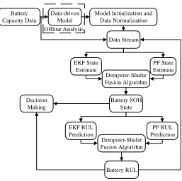
in each state estimator. Figure 3.1 demonstrates the flow chart used in designing

the proposed prognostic system. In our application, we have implemented different

models for EKF and PF, thus demonstrating that our DST fusion technique can

be implemented indepent from state estimation technique and underlying model.

Instead, DST fusion is dependent upon accurate representations of uncertainty

present within the different techniques. In our framework, we could conceivably

fuse any two or more prognostic techniques simultaneously, only being constrained

by the hardware processing capability (e.g. CPU clock speed, parallel computing,

etc.). Thus DST is scalable as necessary to describe the complexities of the unit

under test (UUT).

The nonlinear process model (from cycle k −1 to cycle k) for battery capacity

degradation is described as a hidden Markov model (HMM) by

xk=f(xk−1, uk−1) +wk−1 (3.1)

where xk and xk−1 are the battery capacity state at the current cycle, k, and the

previous cycle, k − 1, f(·) is a nonlinear model describing the battery capacity

degradation, uk−1 is the operating condition, and wk−1 is process noise. The

observation model is

(19)

Data-driven Model PF State Estimate EKF State Estimate Dempster-Shafer Fusion Algorithm Model Initialization and

Data Normalization Data Stream Offline Analysis Battery Capacity Data PF RUL Prediction EKF RUL Prediction Dempster-Shafer Fusion Algorithm Battery SOH State Decision Making Battery RUL

Figure 3.1 Fusion prognostics system diagram.

wherezis the observation vector, which in battery capacity degradation application is

the capacity calculated by Coulomb-counting,h(·) is a nonlinear observation function,

and vk+1 is the measurement noise. Note that process noise ω and measurement v

must be Gaussian in EKF while they can be any non-Gaussian noises in PF.

3.1 Extended Kalman Filter

For state estimation, the KF is known as a linear quadratic optimal filter. This

algorithm is a linear, discrete time, finite dimensional time-varying state estimator

that minimizes the mean-squared error (MSE). Capacity degradation of Li-ion

batteries is a nonlinear process, described with respect to charging-discharging cycles,

for which KF is insufficient and necessitates the use of EKF. The EKF expands the

KF to incorporate non-linear dynamics, by linearizing around the current state, as

(20)

and correction. Both the prediction and correction steps require the calculation

of the partial derivatives (the Jacobian) of f(·) and h(·), which are used for local

linearization, as shown below:

State Jacobian:

Fk=

∂f ∂x _x_ˆ

k−1|k−1,uk−1

(3.3)

Observation Jacobian:

Hk =

∂h ∂x _ˆ_x

k−1|k−1

(3.4)

The prediction step of EKF comprises the following:

1. Project the a priori state at the next time instant (cycle for battery SOH

application) by using the model

ˆ

xk|k−1 =f(ˆxk−1|k−1, uk) (3.5)

2. Project the prediction error covariance, P, ahead

Pk|k−1 =Fk−1Pk−1|k−1Fk−T 1 +Qk−1 (3.6)

where Q is the process noise covariance matrix.

For the correction step of EKF:

1. Compute the Kalman gain, K

Kk=Pk|k−1HkT

HkPk|k−1HkT +Rk

(3.7)

2. Update error covariance, P

Pk|k = (I−KkHk)Pk|k−1 (3.8)

3. Update the state estimate with measurement

ˆ

xk|k = ˆxk|k−1+Kk−1

zk−1−h(xk|k−1)

(21)

Theposteriori estimate provided by Eq. (3.9) provides initial condition for long-term

prediction in RUL calculation. The state models are recursively used to generate

the a priori estimation of battery capacity in all future cycles. These a priori

battery capacity state distributions are compared against the battery capacity failure

threshold to calculate the Time to Failure (TTF) or RUL distribution. Note that since

no measurement available in this long-term prediction, the correction step cannot be

implemented, which will result in increase of uncertainty described in P in 3.6. The

uncertainty must be properly managed to achieve reliable prognosis.

3.2 Particle Filter

One disadvantage of the EKF is that the desired pdf is estimated by a Gaussian,

and as the system under study is not normally distributed, the estimation could

deviate from the actual distribution and diverge [12, 34, 35]. The PF is developed as

a solution for nonlinear random non-Gaussian systems. The algorithm assumes the

process state equations can be effectively modeled as a first-order nonlinear Markov

process in Eqs. (3.1) and (3.2) . The state x and observation z for cycles 1 to k are

defined as

x0:k,{x0, x1, . . . , xk}, z1:k ,{z1, z2, . . . , zk} (3.10)

The PF is also known as a sequential Monte Carlo method for state-space inference.

PF is able to accommodate nonlinearities easily, provided enough particles are used.

The particle filter aims to obtain a set of weighted particles to estimate the battery

capacity based upon a nonlinear model. The algorithm begins with a set ofNparticles

available at cycle k−1 that describe the battery capacity distribution, which is also

the target distribution, denoted as p(x0:k−1|z1:k−1). The objective of filtering is to

obtain a set ofN new particles to approximate the target distribution at cyclek,πk.

To obtain these new particles, a known distribution is chosen by the user to be the

(22)

qk (also known as the importance distribution) as shown,

{x(_0:i)_k}i=1,...,N ∼qk(x

(i)

0:k) (3.11)

and compared against the target distribution. The true distribution is approximated

by a set of N weighted particles, {w_k(i), x_0:(i)_k}i=1,...,N N

X

i=1

w(_ki)φk(x(i)) N→∞

−−−→ Z

φk(x0:k)πk(x0:k)dxk (3.12)

where φk is any πk integrable function and the sum of all weights is 1. To

accommodate the difference between importance distribution and target distribution,

importance sampling set the weights of N particles equal to the ratio between them,

i.e.,

˜

w(x(_0:i)_k) = π(x

(i) 0:k)

qk(x

(i) 0:k)

(3.13)

which is normalized as

w(x(_0:i)_k) = w˜(x

(i) 0:k)

P ˜

w(x(_0:i)_k) (3.14)

With this new set of weights, the target distribution can be approximated as:

π(x0:k) = N

X

i=1

w_k(i)δ(x0:k−x

(i)

0:k) (3.15)

In a simple case of the particle filter, Bootstrap filter, the importance density function

is set as the a priori pdf,

qk(x0:k|x0:k−1) =p(xk|xk−1) (3.16)

In this setting, the weights for the newly generated particles are proportional to the

likelihood of new observations, i.e.

w(_ki) =w_k−(i)₁·p(z1:k|x

(i) 0:k) =w

(i)

k−1·p(zk|x

(i)

k ) (3.17)

In particle filters, degeneracy is a problem that must be addressed. Degeneracy can

(23)

continues to be performed. This leads to a dominance of particles with small weights

describing the distribution. In practice, this results in inaccurate estimation of the

actual state. Degeneracy is addressed by resampling. Resampling effectively replaces

the smaller-weighted particles with larger-weighted particles, so as to describe to true

distribution with higher veracity [36]. Sequential Importance Resampling (SIR) is the

PF implementation chosen for this application due to its robustness. The variance of

the weighted particles generated by the Bootstrap filter is calculated using an effective

sample size:

˜

Neff =

1

PN

i=1(w (i)

k )2

(3.18)

When ˜Neff < Nthreshold, the particles are resampled to eliminate particles with small

weights. The steps in SIR are included in Algorithm 1.

Algorithm 1Sequential Importance Resampling

1: N(i) =jN ·w(_ki₁)k .Identify best particles 2: N =N−P

N(i) . ResampleN particles 3: Nres=

N·w(_ki)−N(i)

N .Resampled particle weights 4: Sres=

n Pi

1N (i) res

o

i=1,...,N .Cumulative sum 5: {u(i)_}

i=1,...,N ∼ U[0,1] . Sample from uniform distribution 6: SORT:u(i) _s.t. _u(i)_{< u}(i+1) _._{Ascending sequential order}

7: fori= 1 :N do .IndexN(i)_{with resampled particles}

8: if u(i)_{< S}(i) res then 9: N(i)=N(i)+ 1

10: end if

11: end for

12:

x(i·N (i)₎

0:k−1

i=1,...,N

∼qk

x0:k|x (i) 0:k−1

.Resampling

3.3 Dempster-Shafer Combination Theory for Fusion

In DST, the concept of belief variables is introduced [37]. Each belief variable is

characterized by its basic belief assignment (bba), m, which can be described as

(24)

A1, . . . , An are the hypotheses, or sets, of interest where each Ai ∈2X, then

m: 2X →[0,1],

n

X

i=1

m(Ai) = 1, m(∅) = 0 (3.19)

Using these bba’s, “Dempster’s Rule” is the fundamental equation governing the

combination of evidence in belief theory [38].

(mi⊕mj)(C) =

P

A∩B=C

mi(A)mj(B)

1−K ; A6=∅ (3.20)

(mi⊕mj)(∅) = 0, (3.21)

K = X

A∩B=∅

mi(A)mj(B), (3.22)

where m is the mass for each hypotheses, i and j are the sources of information,

EKF and PF. C is the output, which is the battery capacity state in the fusion

of diagnosis and battery RUL in the fusion of prognosis. A and B are hypotheses

about the battery capacity and RUL: healthy or faulty. In our application, two other

hypotheses are including to represent the uncertainty.

The sum of the masses in the numerator can be known as the belief measure of

the hypothesis, which is also called the support measure in some literature. The

denominator is called the plausibility measure [39]. The belief and the plausibility

provide confidence bounds, which, when combined as indicated in Eq. (3.20), supply

degrees of belief for the output. Equation (3.21) is the probability mass of the null

set. K represents the mass associated with conflicting evidence. In Bayesian theory,

the resulting probabilities are limited to distribution between the hypotheses, as in

P(A) = 1−P(B). This assumes crisp separation of probabilities between the two

hypotheses, which is not a safe assumption in critical systems. The flexibility of

DST allows for more states to be defined easily. If for instance a Bayesian decision

fusion system is required to utilize two sensors to discern whether a system is healthy

or faulty, and the resulting probabilities are equally divided, the results can be

(25)

defined hypotheses or innacurate sensor information. This level of uncertainty is not

acceptable for online decision-making. DST is a quantitative means of representing

uncertainty. In other words, DST allows for the explicit definition of alternative

scenarios. These new proposed states can be various combinations of the original

states. Shafer’s overview of DST in [26] identified the important assumptions when

approaching an appplication of DST:

1. the assigned masses are subjective in nature, not objective,

2. the sources are independent from one another,

3. the uncertainties within the problem are explicitly represented, and

4. the combination rule is carried out computationally.

The probability masses, as explained above, are not actual probabilities. These are

expected to subjective masses from the perspective of the source. It follows then that

DST will produce meaningless results if source i and source j are dependent upon

one another, and are biased in the same manner. This means that DST cannot be

used in cases of common uncertainty. If proposed states are in direct conflict with

one another, which is mathematically represented by disjoint sets, DST produces a

result of 0, per Eq. (3.21). In the event that sources deviate substantially from one

another, DST will not produce confidence bounds. This is intuitive, since directly

contradictory results cannot be combined by averaging or other methods.

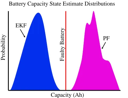
Consider an example using our Li-ion battery system, Fig. 3.2. Notice that

the state estimate pdfs from EKF and PF have no overlap. Considering three

hypotheses, healthy, faulty, or uncertain states, the results from EKF and PF are

directly contradictory. If the below combination rules are applied:

m(F) = mPF(F)mEKF(F)+mPF(F)mEKF(U)+mPF(U)mEKF(F)

1−(mPF(H)mEKF(F)+mPF(F)mEKF(H))

m(U) = mPF(U)mEKF(U)

(26)

m(H) = 1−(m(F) +m(U))

The results of fusion would be as follows:

mEKF(F) = 1 mEKF(H) = 0 mEKF(U) = 0

mPF(F) = 0 mPF(H) = 1 mPF(U) = 0

m(F) = 0 m(H) = 1 m(U) = 0

This result is counterintuitive. However, if a methodology for uncertainty could

be incorporated into the measurement, the results would change drastically. By

considering the variance inherent to EKF and PF as its uncertainty the results are

as follows:

mEKF(F) = 0.7 mEKF(H) = 0 mEKF(U) = 0.3

mPF(F) = 0 mPF(H) = 0.75 mPF(U) = 0.25

m(F) = 0.4 m(H) = 0.525 m(U) = 0.075

These results are much improved. In the previous example, DST essentially

ignores the EKF results, however, by incoporating a rudimentary method of

uncertainty representation, the results are more intuitive. Since the PF has a

slightly tighter variance, DST prodcues a result slightly favoring a healthy battery,

but essentially demonstrates that there is not enough information to conclude a

faulty battery. This result also demonstrates the need for more thorough uncertainty

quantification.

However, many researchers have proposed extensions to DST in an effort to

address the problem posed by strongly conflicting evidence, as presented in [40].

They claim that the normalization factor in Eq. (3.22) has the effect of entirely

ignoring conflict, and attributing associated masses to the null set, Eq. (3.21). When

the upper and lower bounds of DST are interpretted probabilistically, inaccurate

and non-intuitive results are possible, as shown in [41, 42]. This is addressed by

using a discounting function, which is mathematically more rigorous [25, 43]. This

(27)

Capacity (Ah)

Prob

ab

ilit

y

Battery Capacity State Estimate Distributions

Faulty

Battery PF EKF

Figure 3.2 Disjoint sets for Dempster Shafer Fusion

extended framework, the degree of trust attributed to a particular belief function is

defined as 1−αi, where 0 ≤ αi ≤ 1 and i is the belief function associated with a

particular belief measure.

Belαi₍_A_{) = (1}₋_α

i)·Bel(A)

Bel(A) = 1

n(Bel

α1₍_A_{) +}_{. . .}₊_Belαn₍_A₎₎

(3.23)

where:

Belαi₍_A_{) is the discounted belief function}

Bel(A) is the averaged discounted belief function

This discounting technique has been used to formulate another method for

assessing the reliability of two sources, which is explained further in section 4.2.1.

3.4 Uncertainty Representation

In the previous section, the accurate representation of uncertainty is identified as a

critical step to the proper application of DST. A thorough overview of uncertainty

representation is presented in [44]. Uncertainty can be separated into epistemic

and aleatory uncertainty. Aleatory uncertainty describes the natural, unpredictable,

(28)

an estimated magnitude for this uncertainty, but will not reduce it. These are

commonly representated by probability distributions. Whereas, epistemic uncertainty

is a result of incomplete information about a system, its surrounding environment,

or the modeling process. Insufficient experimental data or unmodeled, complex

physical dynamics are examples of epistemic uncertainty. This type of uncertainty

is able to be properly managed. Without sufficiently identifying and modeling

these two categories of uncertainty within an engineered system, this is propagated

throughout the model. This unmodeled uncertainty will yield misleading results.

The DST framework is uniquely able to accomodate and combine both epistemic

and aleatory uncertainty. As uncertainty representation is inherently subjective,

it is important that the designer has sufficient knowledge to distinguish between

the different uncertainty modes, which can involve both qualitative and quantitative

analysis.

3.5 Evaluation Metrics

Different evaluation methods are needed for diagnostics and prognostics. In

this section are presented the different categories of metrics used to validate our

algorithms.

3.5.1 Aging Detection Metrics

The primary goal of fault detection is the early detection of system faults. This

is crucial since the detection of a fault triggers the prognostic algorithm to begin

making predictions. In [33], the TTF metric was used for evaluation. This metric

demonstrates how early the detection algorithm indicates a fault in the system. A

good result is measured by the algorithm which makes earliest fault declaration.

(29)

Figure 3.3 The concept of time-to-failure (TTF).

where kD is the time index at which the fault is detected by diagnostic system.

Figure 3.3 illustrates this. Other metrics include sensitivity, selectivity, area under

the receiver operating characteristic (ROC) curve, and others mentioned in [45, 46].

As this work is primarily focused on enhanced prognostics, we limit our diagnostic

metrics to the earliest TTF generated by each algorithm.

3.5.2 Prognostic Metrics

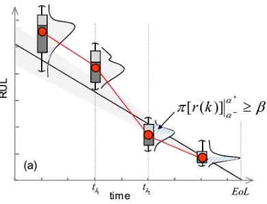
Saxena, et al. introduced several metrics for anlayzing the performance of prognostic

systems [47], and provided further clarifications for using these metrics in [48]. The

concepts presented are successive tests providing quantitative prediction quality. α-λ

performance describes whether a prediction falls within specified limits at certain

times of the life of the failing system. By requiring the prediction to remain in a

specified cone of accuracy, this metric provides a strict requirement for the prognostic

algorithm. In this implementation, we define α-λ accuracy as follows: α×100% of

the ground truth, or baseline, RUL at specific time instance,kλ, which is a time-step

(30)

α = 0.2 and λ = 0.5 would test the prognostic algorithm for 20% accuracy halfway

to EoL after fault detection. This metric can be used to validate both accuracy and

precision performance. This concept is further developed through the use of a β

criterion, as shown in Eq. (3.26). This helps account for the prediction uncertainty,

which is a key factor in this work. The β criterion is defined as the total probability

of RUL predictions being within α bounds at time k. Figure 3.4 shows an example

of α-λ accuracy with β criterion.

(1−α)·r∗(k)≤rl(kλ)≤(1 +α)·r∗(k) (3.25)

where:

l is the lth _{UUT (i.e. Li-ion battery)}

α is an accuracy modifier

λ is a window modifier

kλ =kP +λ(EoL−kP).

π[rl(k)]

α+

α− ≥β

α+ =r∗(k) +α·EoL

α−=r∗(k)−α·EoL

(3.26)

where:

β is total probability in [0,1]

rl₍_k_{) is RUL prediction at time} _k

r∗(k) is baseline RUL prediction at time k.

The output of the metric is binary (Yes or No), stating whether the algorithm

meets the requirement within a specific window. The Relative Accuracy (RA) metrics

provide further means of quantitative comparison, building upon theα-λoutput. RA

measures the tracking (above or below the baseline) that an alogorithm performs for

the chosen λ set. A RA result in the neighborhood of 1 represent a perfect score,

(31)

Figure 3.4 The concept of α-λ accuracy [48].

specific λ. Values above or below 1 indicate late or early estimates, respectively. RA

only uses the expected value of the RUL prediction at kλ, so it is used in addition to

the above α-λ metric with β criterion.

Cumulative RA (CRA) demonstrates the change in accuracy over time, in which

predictions made closer to kEoL are weighted higher than those made closer to kP. A

score close to 1 for CRA represents perfect tracking over the entire λ set. RA and

CRA only use the expected value of the RUL prediction at kλ, so they are used in

addition to the above α-λ metric withβ criterion.

RAl_λ = 1− |r∗(kλ)−r

l₍_k λ)|

r∗(kλ)

(3.27)

CRAl_λ = 1

|`λ| `λ

X

i=1

w(rl(i))RAl_λ (3.28)

where:

w(rl_{) is a weight factor as a function of RUL at all time indices}

`λ is the set of all time indices before kλ when a prediction is made

(32)

Chapter 4 Application with Lithium-ion Batteries

In this section, the proposed approach will be demonstrated in a case study

of the capacity degradation of Li-ion batteries. The battery is a safety-critical

component that provides power to system functions including command, control,

communications, computers, and intelligence. Li-ion batteries are widely used due to

the advantages in higher energy density, longer cycle life, no memory effect, and lower

weight [49]. Since the life and state of the batteries are not directly measurable, state

estimation techniques play an important role in estimating the battery state-of-health

and state-of-charge.

In this implementation, the state-of-health of Li-ion batteries with rated capacity

of 1.1 Ah are used to verify the proposed approach. The charge-discharge cycle of

the battery is conducted with the Arbin BT2000 system under room temperature at

a discharge current of 1.1 A. The charging and discharging of the battery are halted

at the given cutoff voltage. The capacity degradation curve versus charge-discharge

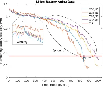
cycle is obtained by Coulomb counting. Figure 4.1 shows the battery aging features

for 4 Li-ion battery UUT, denoted as CS2_35 to CS2_38. The EoL of the Li-ion

batteries is chosen to be 0.35 Ah from the data.

4.1 State Estimation Implementation

For each state estimation technique, a model is develped for use in fault diagnostics

and prognostics (FDP). The diagnostic models are configured for one-step-ahead

(33)

Figure 4.1 Data from run-to-failure test with four Li-ion batteries.

prognostic estimation. The battery is flagged as “aged” once the state estimate is

below the detection threshold (1.03 Ah). This threshold is calculated using the first

10% of the values as a baseline. There is slight debouncing added to the threshhold

to reduce false alarms. Once the Li-ion battery aging is detected, prognosis algorithm

begin generating RUL pdfs in the methods described below.

4.1.1 EKF FDP Implementation

The battery capacity model for EKF is modified from [50] is defined as:

C(k+ 1) =C(k)−p1 ·(p2+p3·k+p4·k2) (4.1)

where C is battery capacity, k is the time index given by cycle number, and p =

[1×10−5_,₃_.₈_×₁₀−5_,₄₅_,₀_._{02] are parameters. The Jacobian is then calculated for}

each iteration of new data. As each new data point becomes available, it is analyzed

(34)

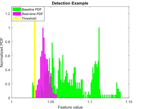
Figure 4.2 Detection is performed by comparing the baseline pdf (healthy battery) and the real-time pdf (based on model and measurement). The threshold is

determined by the probability of false alarm. This figure shows an example of particle filter.

used to adjust the dependence of the state estimate upon the model or upon the

measurements.

Diagnosis

State estimate pdfs are calculated using the EKF linearized mean and the noise

covariances to calculate the spread of the estimate. This pdf is then compared to the

detection threshold, as illustrated in Fig. 4.2. Detection is performed by integrating

from -∞ to the threshold (for a decreasing fault mode like degradation of battery

capacity) or from the threshold to ∞ (for an increasing fault model, such as a crack

growing on a component). Once the probability of detection is greater than or equal

(35)

End of Life Threshold

Cycles ks=0

Current cycle Past system behavior (previous states)

ks= kd[1]

Damage result indices

ks= kd[2] ks= kd[3]

System state/ damage Degradation curves TTF PDF Damage PDF(kd[1])

Damage PDF(kd[2])

PDF of current system state

TTF CDFmax=1

TTF CDFmin=0

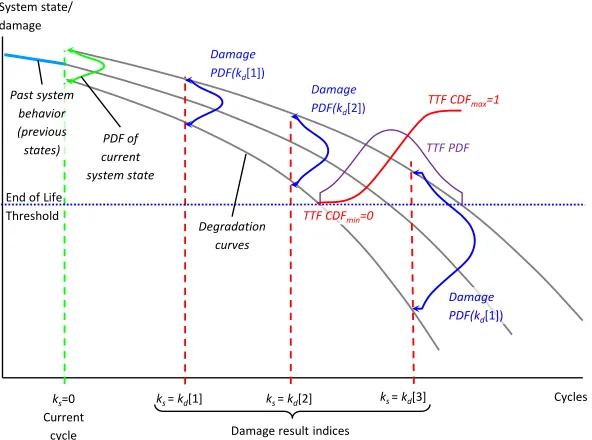
Figure 4.3 The fault progression from EKF over time and the generation of RUL

pdfs from state estimate, or “damage”, pdfs with Gaussian distributions. Uncertainty grows in prognosis since there is no correction step.

Prognosis

Once prognosis is triggered, current state estimate is projected into the future using

the model in Eq. (4.1). Figure 4.3 illustrates the process by which state estimate pdfs

are converted to TTF or RUL distributions. The TTF is estimated using a Gaussian

distribution.

CDFTTF(k) =

Ff

Z

−∞

f(xk|µk, σ2k)dx (4.2)

As the state estimate crosses the EoL threshold, Ff, a cumulative distribution

function (cdf) is generated. Then the pdf of TTF can be calculated from the cdf.

4.1.2 PF FDP Implementation

The battery capacity model for PF is developed from empirical data, and is defined

as:

(36)

where C is battery capacity, k is the time index given by cycle number, p =

[92.5×10−4_,₂_._{9] are parameters,} _u _{is an unknown state, and} _ω _{is model noise. The}

unknown state, u is used to represent dynamics not quantified by the model.

Diagnosis

The PF algorithm uses the model above and performs a one-step-ahead state estimate.

The following model for detection is augmented from the fault dynamic model in Eq.

(4.3).

"

xd,1(k+ 1)

xd,2(k+ 1)

#

=fb

" xd,1(k)

xd,2(k)

#

+n(k) !

xc(k+ 1) = [xc(k)−C(k)]·xd,2(k) +ωk

y(k) =xc(k) +v(k)

where, fb=

        

[1 0]T_, _if

x−[1 0]

T ≤

x−[0 1]

T

[0 1]T, else

(4.4)

is a nonlinear mapping, xd,1 and xd,2 are Boolean states that indicate normal and

faulty conditions, respectively, y(k) is the battery capacity from Coulomb counting,

ω(k) and v(k) are noise signals, and n(k) is i.i.d. uniform white noise. When a fault

is detected, xd,2 = 1. The initial condition is given by

h

xd,1(0) xd,2(0) xc(0)

i

= [1 0 0],

wherexc(0) is the initial battery capacity. With this model, a state estimate pdf is

calculated after SIR has been performed to provide the correct weighting. As detailed

in section 4.1.1, the detection algorithm compares this pdf to the detection threshold

and computes the probability of detection.

Prognosis

Similar to EKF prognosis, once prognosis is triggered, the particles in Eq. (3.15) are

projected into the future using the model in Eq. (4.3). Figure 4.4 illustrates how

(37)

End of Life Threshold

Cycles ks=0

Current cycle Past system behavior (previous states)

ks= kd[1]

Damage result indices

ks= kd[2] ks= td[3]

System state/

damage Degradation

curves

PDF of current system state

TTF CDFmax=1

TTF CDFmin=0

TTF PDF

Figure 4.4 The fault progression from PF over time and the generation of RUL

pdfs from state estimate, or “damage”, pdfs using particles. Uncertainty grows in prognosis since there is no correction step.

particles less than the EoL damage threshold, Ff.

CDFTTF(k) =

N

X

i=1

w_k(i)pfailure|x(_ki)< Ff

(4.5)

4.2 Data Fusion

4.2.1 Uncertainty Quantification

In designing the uncertainty representation, the dataset including all of the Li-ion

battery trajectories over time are investigated. Figure 4.5 shows how aleatory and

epistemic uncertainty are represented separately. In this case,aleatory uncertainty is

evidenced by the random noise in the battery capacity. In our implementation below,

EKF and PF have “noise terms”, which can be tuned to account for this uncertainty

(38)

To quantify this uncertainty, Eq. (4.6) is derived. The spread, S, of the function

is represented by 2·σ2_{, where} _σ2 _{is the variance. If either of the sources exceeds}

the spread limit, Smax, its contribution to the DST combination is ignored. Smax is

defined as 0.3 Ah for battery capacity state in diagnosis, and 300 cycles for battery

EoL in prognosis. The aleatory uncertainty,Ual, is represented as

Ual(k) = S Smax

(4.6)

Although our models include an unknown state to account for the variety of

trajectories, they do not capture all possible variation in trajectory. This

unaccounted-for variation in trajectory is classified as epistemic uncertainty.

Beginning at cycle 400, epistemic uncertainty appears to increase with time. This

uncertainty is quantified in our implementation as a time-varying function, Eq. (4.7),

given as

Uepi(k) = (1−Ual,k)·

1 +e−γ·(k−koff) (4.7)

where:

is the maximum uncertainty, [0,1]

γ is the rate-of-change in uncertainty, [0,1]

koff is the offset cycle at whichUepi reaches ₂

Equation (4.7) indicates that the uncertainty in a given estimator grows over time,

but does not increase beyond a designated maximum. The modified sigmoid function

provides a nice framework to represent bounded uncertainty with a growth rate that

varies with charge-discharge cycle. Forγ = 0, the epistemic uncertainty is assumed to

be constant for all cycles. Since uncertainties must be independent from one another

(as required by the DST framework, the general uncertainty function is modified for

each state predictor, depending upon the experimental performance of each state

predictor at specific instances, Fig. 4.6, which represents experimental testing. EKF

(39)

0 100 200 300 400 500 600 700 800 900 1000 0

0.2 0.4 0.6 0.8 1 1.2

CS2_35 CS2_36 CS2_37 CS2_38 EoL

Aleatory

Epistemic

Figure 4.5 Aleatory and epistemic uncertainty represented for Li-ion battery.

However, as the current cycle k approaches the failure threshold kEoL, both PF and

EKF perform with similar accuracy. This epistemic uncertainty representation can

be improved by performing further experimentation on more Li-ion battery data.

4.2.2 Mass Selection for Healthy and Faulty Battery

Once the uncertainty is properly accounted for, the remaining two states are

considered. The bba for thefaultystate is assigned as shown in Eq. (4.8) for diagnosis

and in Eq. (4.9) for prognosis:

mf(k) =p(failure|xk < η)·(1−Ual,k−Uepi,k) (4.8)

(40)

Figure 4.6 Unmodeled uncertainty functions for each RUL prediction alogrithm.

where η is the fault detection threshold, ξ is the failure threshold when the Li-ion

battery has reached EoL, and p(·) is a probablity function. The healthy state bba

is simply mh(k) = 1−(Ual,k+Uepi,k +mf,k), which satisfies the requirement in Eq.

(3.19) for the sum of the bba’s of all sets be equal to 1.

4.2.3 Combination of Masses

Similar to the example described in section 3.3, Table 4.1 shows the developed

combination table using the bba’s for the four states developed in the above sections.

The green color box area represents the contradictory evidence (i.e. where EKF and

PF estimate directly opposing results for the two primary hypotheses: healthy or

faulty battery state). The purple color box, m(F), contains the bba combinations

where EKF and PF agree with one another. Agreement is quantified in two ways:

1. EKF and PF both believe that the battery is faulty (i.e. m1(µ2)·m2(µ2))

2. Either EKF or PF believes the battery is faulty and the other has a degree of

(41)

The combined uncertainty is represented by the cyan color box, m(U). Equation

(4.10) is the application-specific DST combination for each prediction cycle.

Observations of faulty states have been combined with each of the uncertain states

in this architecture. The separation of uncertainty into separate categories allows

for interesting results. For instance, even though the prediction spread, described

by aleatory uncertainty, Ual in Eq. (4.6), and µ3 in Table 4.1, tends to decrease for

both EKF and PF as the current cycle k approaches kEoL, it is possible for EKF

and PF to deviate significantly from one another. With the addition of the epistemic

uncertainty of modeling error, described by Uepi in Eq. (4.7), and µ4 in Table 4.1,

DST can compensate its fusion using the experimental performance of EKF and PF.

This also mitigates the problem of disjointed sets. The DST algorithm computes Eq.

(4.10) for each cycle.

m(F) =m(µ2)·m(µ2)+m(µ2)·m(µ3)

+m(µ2)·m(µ4)

m(U) =m(µ3)·m(µ3)+m(µ3)·m(µ4)

+m(µ4)·m(µ4)

PF(k) =

P m(F)

1−P

m(µ1)·m(µ2)

PU(k) =

P m(U)

1−P

m(µ1)·m(µ2)

(4.10)

where PF is the belief that a battery fault is detected (diagnosis) or the belief that

the battery capacity has degraded to the EoL (prognosis), and PU is the belief of

uncertainty. For diagnosis, PF is used directly to assess whether the battery capacity

is sufficiently degraded to trigger prognosis.

For each cycle of prognosis, Eq. (4.10) is calculated recursively until k reaches

kEoL. These results produce a cdf, as shown in Fig. 4.7. Notice that the cdf never

reaches “1”. This is representative of the fundamental difference between probabilities

(42)

Table 4.1 The combination of different states within DST framework. m1 and m2

represent mass functions for EKF and PF, respectively. µ1, µ2,µ3, µ4 indciate

healthy state, faulty state, aleatory uncertainty, and epistemic uncertainty, respectively.

PF

Healthy Faulty Uncertainty_al Uncertainty_epi

m₂(μ₁) m₂(μ₂) m₂(μ₃) m₂(μ₄)

EKF

Healthy m₁(μ₁) m₁(μ₁)·m₂(μ₁) m₁(μ₁)·m₂(μ₂) m₁(μ₁)·m₂(μ₃) m₁(μ₁)·m₂(μ₄)

Faulty m₁(μ₂) m₁(μ₂)·m₂(μ₁) m₁(μ₂)·m₂(μ₂) m₁(μ₂)·m₂(μ₃) m₁(μ₂)·m₂(μ₄)

Uncertainty_al m₁(μ₃) m₁(μ₃)·m₂(μ₁) m₁(μ₃)·m₂(μ₂) m₁(μ₃)·m₂(μ₃) m₁(μ₃)·m₂(μ₄) Uncertainty_epi m₁(μ₄) m₁(μ₄)·m₂(μ₁) m₁(μ₄)·m₂(μ₂) m₁(μ₄)·m₂(μ₃) m₁(μ₄)·m₂(μ₄)

not apply to bba’s. Because of the uncertainty quantification, this belief cdf will never

reach one. The belief density function (bdf) is then derived from the belief cdf. In

order to compare the results from DST to the pdfs generated by the EKF and PF

algorithms in prognosis, the bdf is normalized with its maximum value such that the

integral over the range is equal to one, similar to a pdf. Also shown in Fig. 4.7 is the

uncertainty, PU. The uncertainty increases about the combination point, which in

this application is the EoL, while elsewhere, the uncertainty is flat. This is expected

because at the point of combination the normalization denominator varies as EKF

and PF RUL trajectories cross the EoL threshold. Prior to kP, the uncertainty is

(43)

k_P EoL

Figure 4.7 The graph depicts the belief distributions generated by DST fusion for

prognosis. PU is the belief uncertainty and PF is the belief that the battery has

(44)

Chapter 5 Discussion of Results

5.1 Fault Detection Results

Each algorithm calculates change inprobability of failure (PoF) over time. Figure 5.1

shows the PoF after incorporating each algorithm’s uncertainty into its PoF. The PF

provides earlier indication of fault than EKF, but due to its larger uncertainty, DST

“trusts” EKF more. This normalization is calculated as follows:

PoFnorm =PoF·(1−ζ) (5.1)

where ζ is the uncertainty. Using normalized PoF’s, DST is the clear leader, as its

uncertainty is an order of magnitude lower than that of either PF or EKF, as shown

in Tables 5.2 - 5.5. To minimize false alarms, algorithms must detect fault for 3 cycles

before a fault is declared and prognosis is triggered. These values are calculated at

the point of detection for each algorithm, using a detection threshold of 90%. Even

though the inital PoF for EKF and PF are higher initially, they have a higher degree

of uncertainty. Table 5.1 shows the resulting TTFs for each battery at the point of

detectionfor each algorithm. Even though the margin of detection is is low across the

alogorithms, DST demonstrates increased performance over either algorithm on its

own. In practice, DST is used to trigger prognosis since it detects a fault earlier than

(45)

Table 5.1 TTF Comparison

Battery PF EKF DST Longest Window

CS2_35 690 688 694 DST

CS2_36 605 641 657 DST

CS2_37 691 783 793 DST

CS2_38 784 799 814 DST

Table 5.2 PoF and Uncertainty Comparison for CS2_35

Algorithm PoF (%) Uncertainty PoFnorm (%)

EKF 96.5 0.058 90.8

PF 100 0.093 90.7

DST 95.7 0.007 95.0

EKF 98.3 0.052 93.2

PF 100 0.088 91.2

DST 92.7 0.007 92.0

EKF 97.3 0.052 92.2

PF 100 0.098 90.2

DST 93.0 0.006 92.3

EKF 96.2 0.051 91.3

PF 100 0.097 90.3

(46)

Detection threshold

Figure 5.1 Probability of failure detection results, after normalizing PoF with

uncertainty.

5.2 Prognostic Results

Prognosis begins at kP, the point at which the detection algorithms above signal

that the Li-ion battery has aged. RUL is calculated based upon the expected and

mean value for PF and EKF, respectively. Figure 5.2 shows how the mean RUL is

calculated for each measurement. Performance metrics of 95% confidence intervals

(C.I.) are used to calculate theprediction spread,m(µ3), in Table 4.1.

Each dataset is tested and results from α-λ tests are shown in Table 5.6. This

effectively compares how well each algorithm remained within the α-bounds over the

(47)

k

Figure 5.2 The trajectory of PF and EKF prognosis beginning at kP, shown with

confidence bounds.

Table 5.6 α-λ Results with α = 0.3 & β = 0.85

Battery PF EKF DST

CS2_35 36.2% 60.2% 42.0%

CS2_36 84.7% 71.1% 76.3%

CS2_37 89.7% 96.3% 92.3%

CS2_38 83.7% 83.4% 83.1%

for DST lay in between that of EKF and PF for CS2_35 - CS2_37, and performs on

par with EKF and PF for CS2_38.

Figures 5.3 - 5.6 show the α-λ plots (with uncertainty bounds shown). DST

successfully incoporates the uncertainty within EKF and PF. This is especially

evident when EKF and PF RUL predictions are substantially different. Since EKF

and PF are separated from one another, the total uncertainty spread for DST

incorporates these results and produces a wider bdf, even though the expected value

(48)

batteries, RA and CRA are calculated for every cycle, rather than selecting specific

λ’s of interest. As shown in these plots, DST primarily tracks the algorithm with

the highest demonstrated accuracy, which is the desired performance. For battery

CS2_37, this behavior is not observed as prediction are in the neighborhood of the

EoL, kEoL. This can be attributed to the epistemic uncertainty functions. Near

the EoL, PF produces very narrow confidence bounds, though its mean value may

still deviate unacceptably from the baseline, r∗(k). EKF on the other hand does

not produce confidence bounds as tight, and due to the assumption of modeling

uncertainty made in Fig. 4.6, EKF and PF are treated essentially as equals,

with exception to these confidence bounds. Further experimentation may result in

(49)

(a)

(b)

(c)

(d)

Figure 5.3 Results for CS2_35 Li-ion battery. The upper and lower bounds for

each algorithm are shown. (a) EKF α-λ plot, (b) PF α-λ plot, (c) DST α-λ plot,

Improved Simultaneous Estimation of Location and System Reliability via Shrinkage Ideas

University of South Carolina

Scholar Commons

An Application of Dempster-Shafer Fusion Theory

to Lithium-ion Battery Prognostics and Health

Management

John Weddington

Acknowledgments

Abstract

Table of Contents

List of Tables

List of Figures

Chapter 1

Introduction

Chapter 2

Literature Review

Chapter 3

Approach Development

Chapter 4

Application with Lithium-ion Batteries

Chapter 5

Discussion of Results

(a)

(b)

(c)

(d)

(a)

(b)

(c)

(d)

(a)

(b)

(c)

(d)

(a)

(b)

(c)

(d)