THE ANALYSIS OF THE AUSTRALIAN DOLLAR
USING WAVEFORM DICTIONARIES
Shirley Wong, School of Accounting & Finance Footscray Park Campus Victoria University of Technology
PO Box 14428 MCMC, Victoria 8001, Australia
Abstract
Introduction
Many researchers have explored into the area on exchange rates but only limited success has been achieved. Most of these analysis techniques are based on the qualitative approach; the quantitative approach is often implemented with the classical data analysis technique that is ideal for stationary signals (time invariant). However, the real data for the foreign exchange market, using tick-by-tick observations obtained, are no longer accepted to be stationary.
Recently, waveform dictionaries have been accepted as new data analysis tools for non-stationary data and thus applied in the financial market (Ramsey & Zhang 1997). The waveform dictionaries are a new data analysis technique which is comprised of both windowed Fourier transform and wavelet transform (Daubechies 1992). Each waveform is parameterised by location, frequency and scale. The waveform dictionaries can analyse signals that have highly localised structures in either time or frequency space, as well as broadband structures. Waveforms can, in principle, detect everything from shocks represented by Dirac Delta functions, to short bursts of energy within a narrow band of frequencies that occur sporadically, and finally to the presence of frequencies that hold over the entire observed period.
In this paper, waveform dictionaries are used to analyse the trend of exchange rates of four currencies: the U.S. dollar, the Japanese yen, the British pound and the Euro dollar with the Australian dollar.
Methods
Insights are explored using waveform dictionaries to analyse foreign exchange rates. The specific data used were sampled from daily observations collected by the University of British Columbia. The raw data were from 1 February 1998 to 15 April 1999. The four exchange rates examined were the U.S. dollar/Australian dollar, the Japanese yen/Australian dollar, the British pound/Australian dollar, and the Euro/Australian dollar.
Results
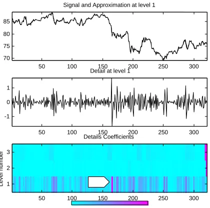
The wavelet transform decomposes the four different signals into time-frequency (scale) maps respectively (see Figures 1 to 4). Figure 1 shows the Japanese yen-Australian dollar exchange rate. The time-frequency map indicates the highest energy location with an arrow.
That is, 153 working days from the starting date 1 February 1998. The d1(detail at level 1) map detects a high spike of the exchange rate on that day. The detail d1 usually shows the high frequency activities of the exchange rate market as the low frequency a1 approximates the trend of the market. Also, the maximum energy level is found at the scale 1 (level 1) of the y-axis. This indicates that the signal nature is smooth and regular. Similar analyses can be applied to the other figures (see Figures 2 to 4).
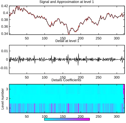
With reference to the signal and approximation in Figure 2, prices will keep to the up-trend or down-trend in the channel if they do not break the upper or lower limit line. If they break the upper limit line and this is confirmed by the following day’s prices, a reversal signal will result which means price will be up. However, the up-trend also needs to be confirmed by the trading day’s volume and indicators.
Referring to the detail in Figure 2, the bargaining powers of the buyers and the sellers are equal. The prices keep fluctuating between the two parallel lines.
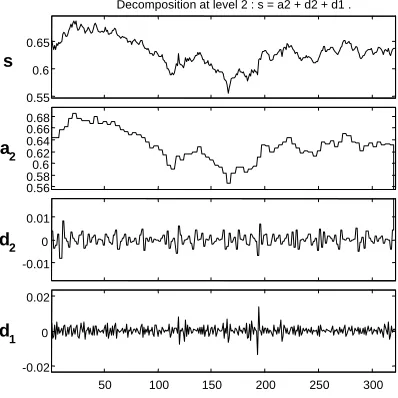
The wavelet features at the details d1, d2 and the approximate a2 for the US$/A$ exchange rate is shown in Figure 5. The signal s is compared to the a2 that indicates the trend of the dollars. D1 shows the high frequency market activities at the sampling rate, 1 datum per 2 days, and d2 shows the lower frequency market activities at half of the frequency of d1, i.e. 1 datum per 4 days. It is shown that the low frequency cycle is approximately 20 working days from the curve d2 in Figure 5.
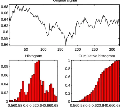
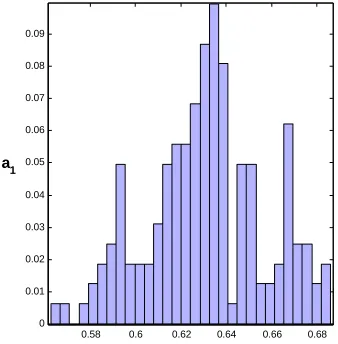
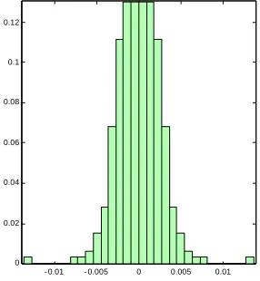
The cumulative frequency of the signal US$/A$ is shown in Figure 6. The highest activity moving the price level is found at US$0.623 within the inter-quartile range. Histograms of the low frequency 'approximate' a1 and the high frequency 'detail' d1 of US$/A$ are shown in Figures 7, 8.
50 100 150 200 250 300 70
75 80 85
Signal and Approximation at level 1
50 100 150 200 250 300
-1 0 1
Detail at level 1
Le v e l num ber Details Coefficients
50 100 150 200 250 300
3
2
1
The colour map (bottom) shows the time and frequency localization of the exchange rate: x-axis shows the working date starting from 1/2/1998; y-x-axis shows the frequency (scale) resolution. The deepest colour location on the map shows the highest energy location.
Figure 2: Euros EU/A$ in 1998
50 100 150 200 250 300
0.5 0.55 0.6
Signal and Approximation(s) at level(s) : 1
50 100 150 200 250 300
-0.01 0 0.01
Detail(s) at level(s) : 1
L e ve l nu m b er Details Coefficients
50 100 150 200 250 300
3
2
Figure 3: GBP/A$ in 1998
50 100 150 200 250 300
0.34 0.36 0.38 0.4 0.42
Signal and Approximation at level 1
50 100 150 200 250 300
-0.01 0 0.01
Detail at level 1
Le
v
e
l nu
m
b
e
r
Details Coefficients
50 100 150 200 250 300
3
2
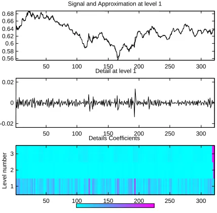
Figure 4: US$/A$ in 1998
50 100 150 200 250 300
0.56 0.58 0.6 0.62 0.64 0.66 0.68
Signal and Approximation at level 1
50 100 150 200 250 300
-0.02 0 0.02
Detail at level 1
L
e
v
e
l nu
m
b
er
Details Coefficients
50 100 150 200 250 300
3
2
Figure 5: Wavelet transform decomposes US$/A$ exchange rate to the wavelet coefficients approximate a2, details d1 and d2
50 100 150 200 250 300 -0.02
0 0.02
d1
-0.01 0 0.01
d2
0.56 0.58 0.6 0.62 0.64 0.66 0.68
a2
0.55 0.6 0.65
s
Figure 6: Cumulative frequency of the signal US$/A$ in 1998
50 100 150 200 250 300 0.56
0.58 0.6 0.62 0.64 0.66 0.68
Original signal
0.560.58 0.60.620.640.660.68 0
0.02 0.04 0.06 0.08
Histogram
0.560.58 0.6 0.620.640.660.68 0
0.2 0.4 0.6 0.8 1
Figure 7: Histogram of the approximate a1 of the signal US$/A$ in 1998
0.58 0.6 0.62 0.64 0.66 0.68 0
0.01 0.02 0.03 0.04 0.05 0.06 0.07 0.08 0.09
Figure 8: Histogram of the high frequency d1 of the signal US$/A$ in 1998
- 0.01 - 0.005 0 0.005 0.01 0
Discussion
The results indicate that the waveform dictionaries can cut non-stationary exchange rate data into different frequency components, for example: scale levels 1 and 2 shown in Figures 1-5. This approach provides an alternative way to extract useful information from spikes or short bursts of energy that may not be sustained throughout the entire period of observation of the data contaminated by noise. Further, the short bursts of energy or spikes of the data may represent short-run bursts of market activity or energy over a narrow range of contiguous frequencies. These localized frequency bursts represent most of the energy of the signal in them but also indicate possible insights into market behaviour. These bursts may be viewed as the dominant market reaction to news. They can be observed clearly at the first difference or detail d1:Dirac Delta functions are found. The median of changes is nearly invariant at zero for d1. This indicates an almost even chance that the price will rise or fall.
To improve forecasting potential, more data and experiments need to be carried out.
Conclusion
Bibliography
Amrhein, E & Guithues, D 1998 Fall, ‘Exchange rates: their importance, purpose and role in translation’, Multinational Business Review, 6(2), pp. 37-43.
Bollerslev, T, Chou, RY, & Kroner, KF 1992, ‘ARCH modelling in finance: a review of the theory and empirical evidence’, Journal of Econometrics, vol. 52, pp. 5-59.
Boothe, P & Glassman, D 1987, ‘The statistical distribution of exchange rates: empirical evidence and economic implications’, Journal of International Economics, vol. 22, pp.297-319.
Brooks, C & Hinich, MJ 1998, ‘Episodic nonstationarity in exchange rates’, Applied
Economics Letters, vol. 5, pp.719-722.
Daubechies, I 1992, Ten lectures on wavelets, Capital City Press.
Henry, O & Olekalns, N 2002, ‘Does the Australian dollar real exchange rate display mean reversion’, Journal of International Money and Finance, pp.651-666.