1/22 Article
Spatial Pattern Oriented Multi-Criteria Sensitivity
Analysis of a Distributed Hydrologic Model
Mehmet C. Demirel 1, 2, *, Julian Koch 1 and Gorka Mendiguren 1, 3, Simon Stisen 1 1 Geological Survey of Denmark and Greenland, Øster Voldgade 10, 1350 Copenhagen, Denmark;
[email protected], [email protected], [email protected]
2 Department of Civil Engineering, Istanbul Technical University, 34469 Maslak, Istanbul, Turkey; [email protected]
3 Department of Environmental Engineering, Technical University of Denmark, 2800 Kgs. Lyngby, Denmark; [email protected]
* Correspondence: [email protected]; [email protected] Tel.: +90-212-285-7624
Abstract: Hydrologic models are conventionally constrained and evaluated using point measurements of streamflow, which represents an aggregated catchment measure. As a consequence of this single objective focus, model parametrization and model parameter sensitivity are typically not reflecting other aspects of catchment behavior. Specifically for distributed models, the spatial pattern aspect is often overlooked. Our paper examines the utility of multiple performance measures in a spatial sensitivity analysis framework to determine the key parameters governing the spatial variability of predicted actual evapotranspiration (AET). Latin hypercube one-at-a-time (LHS-OAT) sampling strategy with multiple initial parameter sets was applied using the mesoscale hydrologic model (mHM) and a total of 17 model parameters were identified as sensitive. The results indicate different parameter sensitivities for different performance measures focusing on temporal hydrograph dynamics and spatial variability of actual evapotranspiration. While spatial patterns were found to be sensitive to vegetation parameters, streamflow dynamics were sensitive to pedo-transfer function (PTF) parameters. Above all, our results show that behavioral model definition based only on streamflow metrics in the generalized likelihood uncertainty estimation (GLUE) type methods require reformulation by incorporating spatial patterns into the definition of threshold values to reveal robust hydrologic behavior in the analysis.
Keywords: mHM, remote sensing, spatial pattern, sensitivity analysis, GLUE, actual evapotranspiration
1 Introduction
Computer models are indispensable to perform costly experiments in an office environment e.g. distributed modeling of water fluxes across the hydrosphere. Physically based distributed hydrologic models have become increasingly complex due to the large number of incorporated parameters to represent a variety of spatially distributed processes. These models are typically calibrated against stream gauge observations i.e. a lumped variable of all hydrological processes at catchment scale. This can cause equifinality problems [1] and poor performance of the simulated spatial pattern of the model since optimizing the water balance and streamflow dynamics are the only concern. To solve this issue the community needs models with a flexible spatial parametrization and calibration frameworks that incorporate spatially distributed observations (e.g. remotely sensed evapotranspiration (ET)).
While LSA methods evaluate point sensitivity in parameter space [7] the GSA covers the entire parameter space and parameter interactions too [8,9]. This is from the fact that, GSA perturbs all parameters simultaneously to assess the inter relations [10]. The most well-known GSA methods are: Sobol’ method [11] and Fourier amplitude sensitivity test (FAST) [12]. The main effects (e.g. first-order sensitivity) and elementary effects, originally described by Morris [13], can be evaluated using both methods. The Morris method has been widely applied in hydrologic modeling. Herman et al. [14] were able to classify parameters of a spatially distributed watershed model as sensitive and not sensitive based on the Morris method with 300 times fewer model evaluations than the Sobol’ approach. The GSA
methods are usually thought to be more appropriate to use in hydrologic applications than LSA methods since hydrological processes are non-linear and the interactions between the parameters have substantial effect on the results. However, the computational cost is crucial in applying the GSA methods in distributed hydrologic modelling [15,16]. The LSA methods gives fast results by assessing only one parameter at a time without interactions between parameters [17]. The local derivatives are however based on a certain initial set in the parameter space.
The foremost objective of our study is to assess the major driving parameters for the spatial patterns of actual evapotranspiration (AET) simulated by a catchment model. Furthermore, we address how the selected initial set of parameters can affect the LSA results and how many initial sets are required for a robust sensitivity analysis. We evaluate parameter sensitivities using a LSA method with random and behavioral initial parameter sets (each containing 100 initial parameter sets). We focus on both spatial patterns of AET over the basin and temporal hydrograph dynamics using multiple performance metrics to evaluate different aspects of the simulated maps and the hydrograph. Streamflow performance of a model has typically been the main concern in conventional model calibrations, whereas improving the simulated spatial pattern during calibration has rarely been targeted [18–24]. A unique feature of our
study is evaluating the model’s sensitivity based on a set of ten spatial metrics that, unlike traditional
cell-to-cell metrics, provide true pattern information. We include an innovative metric which utilizes empirical orthogonal function analysis [21] as well as the fractional skill score [25], among others, to evaluate the simulated spatial patterns. The added value of each metric is assessed based on a redundancy test. This is done to identify the most robust metric(s) with unique information content to apply in a subsequent spatial calibration study.
Recently it has been reported that the VIC model showed difficulty in simulating spatial variability and hydrologic connectivity [20]. Höllering et al [26] used hydrologic fingerprint-based sensitivity analysis using temporally independent and temporal dynamics of only streamflow data. They could identify two major driving parameters for evapotranspiration and soil moisture dynamics in different mesoscale catchments in Germany and reveal their relation to different streamflow characteristics. In our study, we applied the mesoscale hydrologic model (mHM) [27] which can simulate distributed variables using pedo-transfer functions (PTF) and related parameters. Additionally, a recently introduced dynamic ET scaling function (DSF) is used to increase the physical control on simulated spatial patterns of AET [28]. Ultimately, the identified important parameters for simulating both, stream discharge and spatial patterns of AET are used in a very recent model calibration study [28]. The novelty of the current study lies in using sensitivity maps showing difference between initial run and perturbation of a parameter and various spatial metrics to complement conventional SA with spatial pattern evaluation.
2 Materials
Figure 1 Map of Denmark and Skjern River Basin characteristics
2.1 Satellite based data
We use different products from the Moderate Resolution Imaging Spectroradiometer (MODIS) (Table 1) to generate leaf area index (LAI) and AET maps. The data are retrieved from NASA Land Processes Distributed Active Archive Center (LP-DAAC).
Table 1 Source and resolution details of reference satellite data
Variable Description Period Spatial
resolution Remark Source
LAI
Fully distributed 8-day time varying LAI dataset
1990-2014 1 km 8 day to daily
MODIS and Mendiguren et al. [31]
AET Actual
evapotranspiration 1990-2014 1 km daily
MODIS, TSEB
Leaf Area Index (LAI)
The Nadir BRDF Adjusted Reflectance (NBAR) from the MCD43B4 product is used to calculate the normalized vegetation index (NDVI) [32]. Subsequently the dataset are smoothed using a temporal filter available in the TIMESAT code [33,34]. Due to the low data availability of the MODIS LAI product at the latitudes of the study site during some periods of the year we derive a new empirical LAI equation based on the NDVI, Eq. (1).
𝐿𝐴𝐼 = 0.06335.524 ∙𝑁𝐷𝑉𝐼 (1)
Using different equations for different land cover types is possible. However, imposing a land cover map on the remote sensing inputs can predispose the maps to show a spatial pattern controlled by land cover. To minimize this effect, we decided to apply a single equation to derive the LAI i.e. established based on the most abundant land cover type (agricultural) in the study area. The derived 8-day LAI product is later linearly interpolated to obtain daily LAI values for each pixel, which we find suitable for the study area, because temporal variability is limited at this time scale.
Actual Evapotranspiration (TSEB)
The Two Source Energy Balance (TSEB) model developed by Norman et al. [38] based on Priestly-Taylor approximation [39] is incorporated in this study to estimate AET based on MODIS data. The model inputs are solar zenith angle (SZA) and land surface temperature (LST) as well as height of canopy and albedo levels all derived from MODIS based observations. Other climate variables of incoming radiation and air temperature are retrieved from ERA interim reanalysis data [40]. One-at-a-time sensitivity analysis [41] of the TSEB model revealed that LST is the most sensitive parameter for AET (results not shown here). The TSEB model output was evaluated against field observations of eddy fluxes over three different land cover types before deriving the final maps of AET. The main purpose of including the remote sensing based AET estimations is to evaluate the spatial pattern performance of the model data during the growing season. All data were averaged across all years for calibration and validation periods to six monthly averaged spatial maps from April to September. This is from the fact that uncertainty is inevitable in the individual daily estimates of AET whereas the monthly maps show the general monthly patterns which are more robust. We refer to this this AET data as reference data to evaluate mHM based simulations of AET. We chose reference instead of observation, as the data are not purely observed but an energy balance model output using satellite observations.
2.2 Hydrologic model
The multiscale Hydrologic Model (mHM) has been developed as a distributed model delivering different outputs and fluxes at different model scales [27]. The direct runoff, slow and fast interflow and base flow are calculated for every grid cell. Finally, the runoff is routed through the basin domain using Muskingum flood routing method. The model applies pedo-transfer functions to regionalize soil parameters and is easily set-up for different platforms, e.g. Mac, Linux and Windows. The model contains 53 parameters for calibration. The study by Samaniego et al. [27] is the key reference describing model formulation and parameter description.
Meteorological input at different spatial scales can be handled internally by the model. This underlines the flexibility of mHM which operates at three spatial scales: morphologic data scale (L0), model scale (L1) and coarse meteorological data (L2). The model scale, i.e. L1, can have any value between L0 and L2. In our case, the Skjern model runs at daily time scale at 1x1 km resolution whereas the soil inputs have 250x250 m resolution. The meteorological data sets, i.e. P, ETref and Tavg, were resampled from 10-20 km resolution to 1x1 km [28].
Parameter Unit Description Initial value**
Lower bound
Upper Bound
ETref-a - Intercept 0.95 0.5 1.2
ETref-b - Base Coefficient 0.2 0 1
ETref-c - Exponent Coefficient -0.7 -2 0
**Recommended initial values for calibration only. Different initial values are tested in our sensitivity analysis framework.
3 Methods
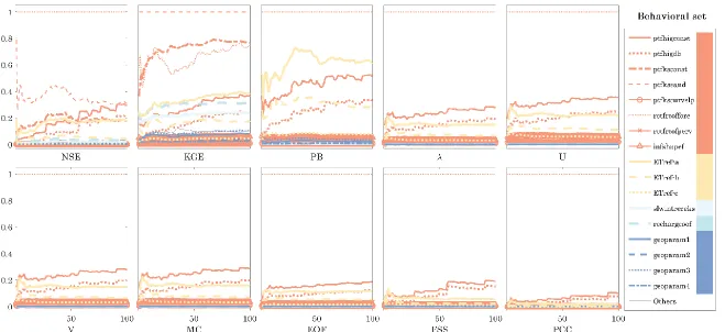
In this study, we applied the Latin-hypercube sampling strategy combined with a local sensitivity analysis approach [17]. We test ten sophisticated performance measures (hereinafter called objective functions) to identify most important parameters. Three of these metrics, i.e. Nash-Sutcliffe Efficiency (NSE, Nash and Sutcliffe [42]), Kling-Gupta Efficiency (KGE, Gupta et al., [43]) and percent bias (PB), focus on simulated streamflow, whereas the remaining objective functions focus on the spatial distribution of AET (Table 3). Although PB is included in KGE equation, the PB that reflects errors in the water balance is evaluated separately to consider volume error in addition to the streamflow timing.
Table 3 Overview of the ten metrics which are used in the sensitivity analysis. First three metrics are regarding time series of streamflow while the latter seven are used to evaluate spatial patterns of AET.
Description Best
value
Abbrev
iation Group Reference
Nash-Sutcliffe Efficiency 1.0 NSE Streamflow [42]
Kling-Gupta Efficiency 1.0 KGE Streamflow [43]
Percent Bias 0.0 PB Streamflow
Goodman and Kruskal’s Lambda 1.0 Spatial pattern [44]
Theil’s Uncertainty coefficient 1.0 U Spatial pattern [45]
Cramér’s V 1.0 V Spatial pattern [46]
Map Curves 1.0 MC Spatial pattern [47]
Empirical Orthogonal Function 0.0 EOF Spatial pattern [21]
Fraction Skill Score 1.0 FSS Spatial pattern [25]
Pearson Correlation Coefficient 1.0 PCC Spatial pattern [48]
3.1 Objective functions focusing on spatial patterns
W/m2. The two units are closely related, but vary in range, therefore applying bias insensitive metrics is inevitable.
Goodman and Kruskal’s lambda
Goodman and Kruskal’s lambda (𝜆) is a similarity metric for contingency tables. It has an optimal value of one indicating perfect match and lowest value of zero indicating no overlap [50]. 𝜆 is calculated as:
𝜆 =∑ 𝑚𝑎𝑥𝑗(𝑐𝑖𝑗)
𝑚
𝑖=1 +∑𝑚𝑖=1𝑚𝑎𝑥𝑗(𝑐𝑖𝑗)−𝑚𝑎𝑥𝑗(𝑐+𝑗)−𝑚𝑎𝑥𝑖(𝑐𝑖+)
2𝑁−𝑚𝑎𝑥𝑗(𝑐+𝑗)−𝑚𝑎𝑥𝑖(𝑐𝑖+) (2)
Where N is the total number of grids; m and n are the number of classes in the observed and simulated maps to be compared. cij is the grid numbers for the class i in first map (A) and to class j in the second map (B); 𝑐𝑖+ is the grid numbers contained in category i in map A, 𝑐+𝑗 is the grid numbers contained in category j in map B; 𝑚𝑎𝑥𝑖(𝑐𝑖+) is the grid numbers in the modal class of map A, i.e. the class with largest number of grids; and 𝑚𝑎𝑥𝑗(𝑐𝑖𝑗) is the number of class in map B with a given class of map A.
Theil’s Uncertainty coefficient
Theil’s Uncertainty(U)is a measure of percent reduction in error. It is also known as average mutual information [50]. It yields the same value when the reference map is A or B i.e. symmetric; therefore, a reference does not need to be defined. Unlike 𝜆 which accounts for modal class, Theil’s U considers the whole distribution of the data. It is based on entropy, joint entropy and average mutual information [45,49]. The information content (entropy) of map A is calculated as
𝐻(𝐴) = − ∑ 𝑐𝑖+
𝑁 log (
𝑐𝑖+
𝑁) 𝑚
𝑖=1 . (3)
The same notation as 𝜆 is used for Theil’s U equation below. Similarly for map B:
𝐻(𝐵) = − ∑𝑐+𝑗
𝑁 𝑙𝑜𝑔 (
𝑐+𝑗
𝑁)
𝑚
𝑗=1
. (4)
𝐻(𝐴, 𝐵) = − ∑ ∑𝑐𝑖𝑗
𝑁𝑙𝑜𝑔 (
𝑐𝑖𝑗
𝑁)
𝑛
𝑗=1 𝑚
𝑖=1
. (5)
The shared information by map A and B is estimated by average mutual information I(A;B) based on the entropy of two maps minus the joint entropy:
𝐼(𝐴; 𝐵) = 𝐻(𝐴) + 𝐻(𝐵) − 𝐻(𝐴, 𝐵). (6)
The uncertainty coefficient is then calculated as:
𝑈 = 2 ∙ 𝐼(𝐴; 𝐵)
𝐻(𝐴) + 𝐻(𝐵). (7)
Cramér’s V
Cramér’s V is a metricbased on Pearson’s 𝑋2 statistic calculated from the contingency table of the map A and B [46]. Recently, Speich et al. [49] used this metric to assess the similarity of different bivariate maps for Switzerland. In their case the variable pairs snowmelt and runoff as well as precipitation and PET, have been selected to describe the water balance in Swiss catchments. The 𝜒2 statistics can be calculated by
𝜒2= ∑ ∑(𝑐𝑖𝑗− 𝑐𝑖+𝑐+𝑗/𝑁)
2
𝑐𝑖+𝑐+𝑗/𝑁
𝑛
𝑗=1 𝑚
𝑖=1
(8)
with using the same notation of 𝑐𝑖𝑗 , 𝑐𝑖+ and 𝑐+𝑗 as for the metrics above. In addition, m and n shows the number of grids in map A and B, respectively. 𝜒2 yields always non-negative values. Zero values only appear in the case when 𝑐𝑖𝑗= 𝑐𝑖+𝑐+𝑗/𝑁.The zero value hence indicates no similarity between the map pairs. There has been different modifications of 𝜒2 [50] but the simplest and most widely used form has been proposed by Cramér [46]. V is a transformation of 𝑋2 as shown below:
𝑉 = √ 𝜒
2
In an earlier study, Rees [50] used Cramér’s V together with two other categorical association metrics (U and 𝜆) to assess the similarity of two thematic maps from Landsat images. All three metrics, investigated in that study, appeared to work well as they produced significantly high values for the maps that are reasonably similar and low values for those maps that obviously differ. Rees [50]
recommended to use Cramér’s V for three reasons: 1) this metric is relatively simple to calculate, 2) it is symmetric giving the same value when the reference map is A or B, 3) it performs slightly better than U and 𝜆 in discriminating between two different maps or approving two similar maps.
Mapcurves
Mapcurves (MC) is a measure of goodness-of-fit (GOF) indicating the degree of match between two categorical maps [49]. It has an optimal value of one whereas the lowest value is zero. For each pair of classes (i, j), between the two maps A and B, the algorithm calculates GOF using the following equation:
𝐺𝑂𝐹𝑖𝑗=𝑐𝑖𝑗
𝑐𝑖+ 𝑐𝑖𝑗
𝑐+𝑗 (10)
In the following equations, the equations are presented for class A (i.e. index i), as the category A represents observed maps and B indicates simulated maps (i.e. index j). Thus the calculation for class B is analogous. The GOF values are added up for each group of the observed map (A):
𝐺𝐴,𝑖= ∑ 𝐺𝑖𝑗
𝑛
𝑗=1
(11)
Where n is the grid numbers in the map (A). Note that the size of maps should match each other for this comparison. The GOF values are organized in ascending order to estimate the vector 𝐺𝐴′. The values 0 and 1 are included in the series of 𝐺𝐴′ to integrate the function later. The length of 𝐺
𝐴′ is hence m+2. For each GOF value i 𝐺𝐴′, the MC is calculated as a segment of classes that have a GOF more than or equal to i:
𝑓𝐴(𝑖) =∑ [𝐺𝐴,𝑘≥ 𝑖]
𝑚 𝑘=1
𝑚 ; 𝑖 𝜖 𝐺𝐴
′ (12)
The MC value is then calculated by integrating f(x) between zero and one. A trapezoid rule is applied as follows to calculate the area under the curve. It has a best value of one.
𝑀𝐶𝐴= ∑ (𝐺𝐴,𝑖+1′ − 𝐺𝐴,𝑖′ ) 𝑛
𝑖=1
𝑓𝐴(𝑥 + 1) +
(𝐺𝐴,𝑖+1′ − 𝐺
𝐴,𝑖′ ) (𝑓𝐴(𝑥 + 1) − 𝑓𝐴(𝑥))
Empirical Orthogonal Functions
The Empirical-Orthogonal-Functions (EOF) analysis is a frequently applied tool to study the spatio-temporal variability of environmental and meteorological variables [51,52]. The most important feature of the EOF analysis is that it decomposes the variability of a spatio-temporal dataset into two crucial components i.e. time invariant orthogonal spatial patterns (EOFs) and a set of loadings that are time variant [28]. Perry et al. [51] give a brief description of the mathematical background of the EOF analysis. The EOF based similarity score (SEOF) at time x is formulated as:
𝑆𝐸𝑂𝐹𝑥 = ∑ 𝑤 𝑖|(𝑙𝑜𝑎𝑑𝑖 𝑠𝑖𝑚(𝑥)− 𝑙𝑜𝑎𝑑 𝑖 𝑜𝑏𝑠(𝑥))| 𝑛 𝑖=1 (14)
where n is the number of EOFs and wi, represents the covariation contribution of the i’th EOF. In our study, we focus on the overall AET pattern performance and thus we average SEOF from the individual months of the growing season into a single overall skill score.
Fractions Skill Score
Roberts and Lean [25] introduced the fractions skill score (FSS) to the atmospheric science community to establish a quantitative measure of how the skill of precipitation products varies for different spatial scales. Fractions relate to occurrences of values exceeding a certain threshold at a given window size (scale) and are compared between model and observation at individual grids. Most commonly, the thresholds represent percentiles which have the purpose to eliminate any impact of a potential bias. Hence, FSS assesses the spatial performance of a model as a function of threshold and scale and has been implemented by Gilleland et al. [53], Wolff et al. [54] and others to spatially validate precipitation forecasts. In summary, the following steps are performed during the FSS methodology: (1) truncate the observed A and simulated B spatial patterns into binary patterns for each threshold of interest, (2) compute fractions A(n) and B(n) within a given spatial scale n based on the number of grids that exceed the threshold and lie within the window of size n by n and (3) estimate the mean-squared-error (MSE) and standardize it with a worst-case MSE that returns zero spatial agreement between A and B (MSEref). The MSE is based on all grids (Nxy) that define the catchment area with dimension Nx and Ny. For a certain threshold the FSS at scale n is given by:
𝐹𝑆𝑆(𝑛)= 1 − 𝑀𝑆𝐸(𝑛)
𝑀𝑆𝐸(𝑛)𝑟𝑒𝑓 (15)
where 𝑀𝑆𝐸(𝑛)= 1 𝑁𝑥𝑦∑ ∑[𝐴(𝑛)𝑖𝑗− 𝐵(𝑛)𝑖𝑗] 2 𝑁𝑦 𝑗=1 𝑁𝑥 𝑖=1 (16) and 𝑀𝑆𝐸(𝑛)𝑟𝑒𝑓= 1 𝑁𝑥𝑦
[∑ ∑ 𝐴(𝑛)𝑖𝑗2
𝑁𝑦
𝑗=1 𝑁𝑥
𝑖=1
+ ∑ ∑ 𝐵(𝑛)𝑖𝑗2
𝑁𝑦
𝑗=1 𝑁𝑥
𝑖=1
] (17)
latter (5 km). In addition, the 5th and 95th percentiles, that represent the top and bottom 5% of AET grids, are assessed at 15 km scale. The average of these six percentiles is used as the overall FSS score.
3.2 Latin-hypercube sampling one-factor-at-a-time sensitivity analysis
We used Latin-hypercube (LH) sampling in combination with a local sensitivity analysis method. This is an integration of a global sampling method with a local SA method changing one factor at a time (OAT). In other words, one perturbation at a time depends on the local derivatives based on a certain initial point in the parameter space [17]. A similar design based on random perturbation at a time following trajectories was firstly proposed by Morris [13]. SA based on Monte Carlo simulation is robust but requires a larger number of simulations. Alternatively, the LHS is based on a stratified sampling method that divides the parameter values into N strata with probability of occurrence having a value of 1/N. This feature leads to a more robust sensitivity analysis with a given number of initial values [17]. Here, we test whether behavioral initial parameter sets result in different parameter identification compared to random initial parameter sets. In addition, we use 100 different initial sets to assess if/when the accumulated relative sensitivities become stable. We can then evaluate how many initial samples were required to get a robust results using LHS-OAT.
4 Results
4.1 Exploration of spatial metrics characteristics
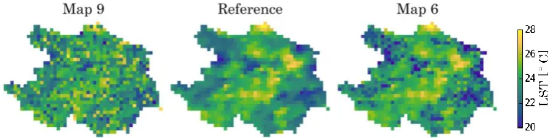
The spatial performance metrics are examined to gain more insight in their reliability and to understand whether any of them provides redundant information. This is an important step before including them into the sensitivity analysis and model calibration, because the ability to discriminate between a good and a poor spatial pattern performance is an essential characteristic of a metric. We compared 12 synthetic land surface temperature (LST) maps of a subbasin of Skjern (~1000km2), i.e. all perturbed differently, with a reference LST map using the spatial metrics applied in this study. The details about the applied perturbation strategies can be found in Table 1 of Koch et al. [21]. In that study, Koch et al. [21] conducted an online based survey with the aim to use the well trained human perception to rank the 12 synthetic LST maps in terms of their similarity to the reference map. The obtained results were subsequently used to benchmark a set of spatial performance metrics. The same procedure is incorporated in this study to get a better understanding of the metrics selected for this study. We included the survey results in our study and assessed the coefficient of determination R2 between the human perception and the spatial metrics. This helps to differentiate between metrics that contain redundant and those with unique information content. Figure 2 shows two distinct examples, i.e. one noisy perturbation and one slightly similar map to the reference map, to better explain the results presented in Table 4, that summarizes the spatial scores for the 12 maps sorted based on the survey similarity index (last column).
Map 9 is ranked as the second least similar map as compared to the reference map. Map 10 that is perturbed with an overall bias of +2 is ranked as a perfect agreement by all metrics. This confirms that all of our spatial metrics are bias insensitive. In addition, map 1 is identified as the most similar map to the reference map by the human perception and all other metrics.
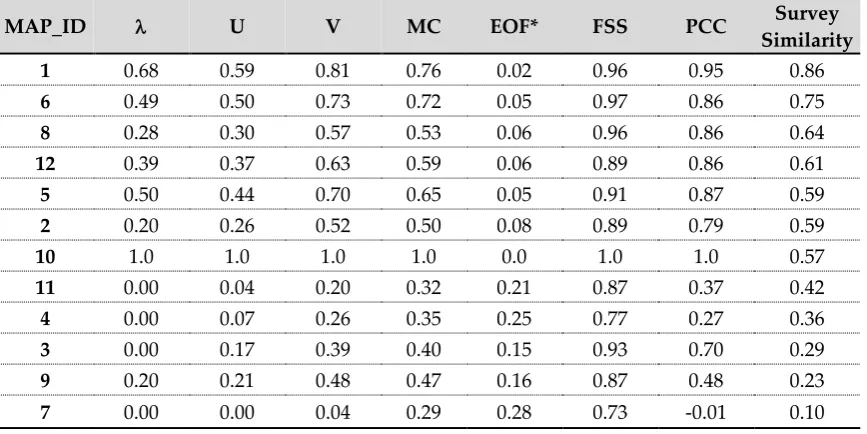
Table 4 Comparison of 12 perturbed maps [21] based on spatial metrics. The first seven columns presents the metrics used in this study while the last column gives the survey similarity reported in Koch et al. [21]. Map 1 has the highest similarity which means that it is the most similar map to the reference while map 7 is the least similar.
MAP_ID U V MC EOF* FSS PCC Survey
Similarity
1 0.68 0.59 0.81 0.76 0.02 0.96 0.95 0.86
6 0.49 0.50 0.73 0.72 0.05 0.97 0.86 0.75
8 0.28 0.30 0.57 0.53 0.06 0.96 0.86 0.64
12 0.39 0.37 0.63 0.59 0.06 0.89 0.86 0.61
5 0.50 0.44 0.70 0.65 0.05 0.91 0.87 0.59
2 0.20 0.26 0.52 0.50 0.08 0.89 0.79 0.59
10 1.0 1.0 1.0 1.0 0.0 1.0 1.0 0.57
11 0.00 0.04 0.20 0.32 0.21 0.87 0.37 0.42
4 0.00 0.07 0.26 0.35 0.25 0.77 0.27 0.36
3 0.00 0.17 0.39 0.40 0.15 0.93 0.70 0.29
9 0.20 0.21 0.48 0.47 0.16 0.87 0.48 0.23
7 0.00 0.00 0.04 0.29 0.28 0.73 -0.01 0.10
*Highest EOF value is zero for similar maps.
Following the R2 values in Table 5, 72.2% of the variance in the human perception is explained by the EOF analysis. The PCC, V and FSS metrics also perform well in discriminating spatial maps with respect to the human perception as benchmark. However, the U metric explains the lowest variance (40.9%) which indicates that it should not be included in the model calibration, because we trust the well trained human perception as a reference. Moreover, the spatial metrics, i.e. , U, V and MC, are highly correlated (italic fonts in Table 5). All are based on transforming the data into a three category system, which results in redundancy between the four given metrics. This shows that not all of them are required for model calibration. However, we will still evaluate the sensitivity results based on all given spatial metrics in the following sections.
Table 5 Coefficient of determination (R2) between spatial metrics and survey similarity. Bold values mark metrics with highest ability to reproduce survey similarity. Italic values highlight spatial metrics which are highly correlated.
R2 score U V MC EOF FSS PCC Survey Similarity
1 0.97 0.88 0.97 0.71 0.51 0.59 0.46
U 1 0.90 0.99 0.72 0.59 0.63 0.41
V 1 0.93 0.90 0.72 0.85 0.59
MC 1 0.77 0.61 0.67 0.49
EOF 1 0.79 0.96 0.72
FSS 1 0.84 0.52
PCC 1 0.69
4.2 Latin-hypercube sampling one-factor-at-a-time sensitivity analysis
In this study, we apply LHS-OAT sensitivity analysis with 47 parameters using both random and behavioral sets of initial parameter values. Initially we selected 100 random initial parameter sets using the lower and upper limits of the parameters. Subsequently, we generate 10,000 random initial samples to select 100 behavioral sets among these. For that we start running each of the 10,000 random set, one at a time, and evaluate the simulated discharge. We continue the model runs until we reach 100 behavioral sets that all result in NSE above 0.5. This is from the fact that we are interested in investigating only the plausible region of the parameter space as we know the calibration will never end up outside this region in either way. We also ensure that the selected 100 behavioral sets are uniformly distributed to the different probability bins since we tested only the first ~2400 random initial parameter sets to have 100 behavioral sets.
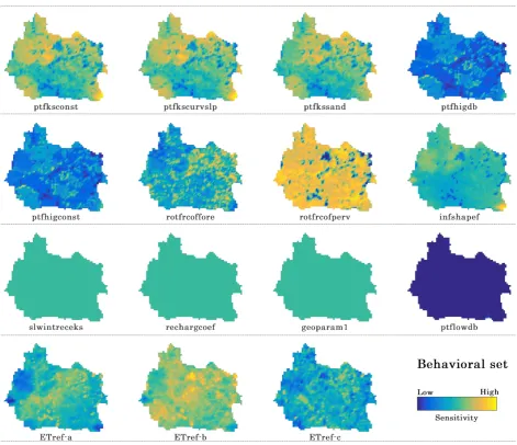
Figure 4 shows the average of 100 maps where each reflects the impact of a perturbation per
parameter based on the 100 behavioral (NSE > 0.5) parameter sets as initial points. Each of these 100 perturbation maps (sensitivity maps) are calculated as absolute difference between the initial run and
the perturbation that is further normalized by the initial run i.e. NMAD (%) = abs(perturbation-initial) / initial. We then use the average of 100 runs as a final sensitivity map. The maps in Figure 4 are informative in several ways. First, they show that some of the parameters have a uniform (light green
map) or no effect (dark blue map) on the spatial pattern distribution, whereas other parameters have a high control on spatial variability (e.g rotfrcofperv, ptfkssand and ETref-a). Second, we can recognize
different patterns on the maps such as land cover patterns (see Figure 1) from root fraction maps (especially the one for pervious areas), LAI patterns from ETref-c map and soil patterns from
pedo-transfer function maps (e.g. ptfksconst). The geoparam 2, 3 and 4 parameters are also identified as sensitive influencing streamflow dynamics (see KGE at Figure 3). However, their maps are not shown
at Figure 4 as they are similar to the map for geoparam 1 (uniform effect). Further, the map for the ptflowdb parameter is completely dark blue showing that it has no effect on the simulated spatial pattern of AET.
Figure 4. Average of 100 sensitivity maps (entire Skjern basin) based on the difference between 100
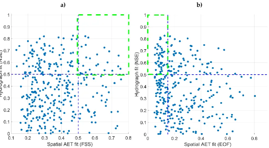
4.3 Random parameter sets based on the 17 sensitive parameters evaluated against NSE and FSS
a) b)
Figure 5. Scatter plot of 329 (NSE>0.0) model runs from a total of 1700 random parameter sets as a
function of spatial fit a) FSS b) EOF between remote sensing actual evapotranspiration and simulated actual evapotranspiration from mHM. Green-box in both figures show the new behavioral regions
when spatial and temporal thresholds are applied together.
5 Discussion
In this study, we identified important parameters for streamflow dynamics and spatial patterns of AET by incorporating different spatial and temporal performance metrics in a LHS-OAT sensitivity analysis combined with spatial sensitivity maps. We first analyzed the suitability of spatial performance metrics for sensitivity analysis. The results suggest that a good combination of performance metrics that are complimentary should be included in a sensitivity analysis. Most importantly, the metrics should be able to separate similar and dissimilar spatial patterns. We concluded this by benchmarking a set of performance metrics against the human perception, which is a reliable and well trained reference for comparing spatial patterns. Furthermore, redundant metrics need to be identified and excluded from the analysis.
Another important point is that the modeler has to select or design a model parametrization scheme that allows the simulated spatial patterns to change while minimizing the number of model parameters. Otherwise the efforts towards a spatial model calibration will be inadequate. Here, the mHM model is selected due to its flexibility through the pedo-transfer functions.
Once the appropriate spatial performance metrics and model are selected, model evaluation against relevant spatial observations can be conducted. Such modelling schemes can be easily incorporated with any parameter sensitivity analysis. In our study, the identified parameters that are sensitive to either streamflow or spatial patterns will be used in a subsequent calibration framework. With this study, we ensure that we select the best combination of objective functions for model calibration and simultaneously reduce the computational costs of model calibration by reducing the number of model parameters.
5.1 Utility of the multi-criteria spatial sensitivity analysis
incorporated different random and behavioral initial sets in our study. This makes the combined approach simple and robust when used with appropriate multiple metrics. It should be noted that LHS-OAT has been validated in different study areas [3,17]. Although the parameter interactions are not evaluated explicitly, the identified parameters seem to be the most important and relevant parameters for calibration. This might stem from the fact that parameters in mHM are not highly interacting with each other as already shown in Cuntz et al. [16]. The resultant maps at Figure 4 are instrumental to decide which parameter has spatial effect on the results. The average accumulated relative parameter sensitivities become stable, i.e. unchanging parameter ranking, after ~20 initial parameter sets used in LHS-OAT. This corresponds to 940 model simulations (20 x 47) including 47 mHM parameters evaluated in LHS-OAT. These are much less number of runs as compared to first
and second order sensitivity analysis based on Sobol’ requiring minimum 104 - 105 model simulations [58,59]. The gain in computational costs is mostly done to the fact that we are not mainly interested in quantitative sensitivity indexes rather than the importance ranking of the model parameters.
6 Conclusions
The effect of hydrologic model parameters on the spatial distribution of AET has been evaluated with LHS-OAT method and maps. This is done to identify the most sensitive parameters to both
streamflow dynamics and monthly spatial patterns of AET. To increase the model’s ability on
changing simulated spatial patterns during calibration, we introduced a new dynamic scaling function using actual vegetation information to update reference evapotranspiration at the model scale. Moreover the uncertainties arising from random and behavioral Latin-hypercube sampling are addressed. The following conclusions can be drawn from our results:
• Based on the detailed analysis of spatial metrics, the EOF, FSS and Cramér’s V are found to
be relevant (non-redundant) pair for spatial comparison of categorical maps. Further, the PCC metric can provide an easy understanding of map association although it can be very sensitive to extreme values.
• Based on the results from sensitivity analysis, the vegetation and soil parametrization mainly control the spatial pattern of the actual evapotranspiration. Besides, the interception, recharge and geological parameters are also important for changing streamflow dynamics. Their effect on spatial actual evapotranspiration pattern is substantial but uniform over the basin. For interception the lacking effect on the spatial pattern of AET is due to the exclusion of rainy day in the spatial pattern evaluation.
• More than half of the 47 parameters included in this study have either little or no effect on simulated spatial patterns, i.e. non-informative parameters, in the Skjern basin with chosen setup. In total, only 17 of 47 mHM parameters are selected for a subsequent spatial calibration study.
• The sensitivity maps are consistent with parameter types as they reflect land cover, LAI and soil maps of the Skjern basin.
• Combining NSE with a spatial metric strengthens the physical meaningfulness and robustness of selecting behavioral models.
Our results are in line with the study by Cornelissen et al. [22] showing that the spatial parameterization directly affects the monthly AET patterns simulated by the hydrologic model. Further, Berezowski et al. [3] used a similar sort of Latin-Hypercube One-factor-At-a-Time algorithm for sensitivity analysis of model parameters affecting simulated snow distribution patterns over Biebrza River catchment, Poland. However, to our knowledge this is the first study incorporating sensitivity maps with wide range of spatial performance metrics. The LHS-OAT method is easy to apply and informative when used with bias-insensitive spatial metrics. The framework is transferrable to other catchments in the world. Even other metrics can be added to the spatial metric group if not redundant with the current ones.
the use of these metrics. The general consensus threshold for streamflow NSE is 0.5, however, this threshold is also arbitrary and slightly differs from one study to another. It is anticipated that once the spatial metrics are more often used in the hydrologic practices, the expertise will grow in identifying suitable performance metrics and threshold value for a satisfying spatial performance. Particularly for the GLUE type uncertainty analysis methods and other model calibration frameworks, a new spatiotemporal perspective for behavioral model definition is indispensable.
Acknowledgments: The authors acknowledge the financial support for the SPACE project by the Villum Foundation (http://villumfonden.dk/ ) through their Young Investigator Program (grant VKR023443). The first author is supported by Turkish Scientific and Technical Research Council (TÜBİTAK grant 118C020). We also thank Manuel Antonetti and Massimiliano Zappa from Swiss Federal Institute WSL for providing the R codes to estimate three spatial indices, i.e. Goodman and
Kruskal’s Lambda, Theil’s U and Cramér’s V. We also acknowledge Emiel E. van Loon from
University of Amsterdam who provides the R code to calculate Mapcurves index at http://staff.fnwi.uva.nl/e.e.vanloon/code/mapcurves.zip. The code for the EOF analysis and FSS is freely available from the SEEM GitHub repository (https://github.com/JulKoch/SEEM). The repository also contains the maps used in the spatial similarity survey and the associated similarity rating based on the human perception. The TSEB code is retrieved from https://github.com/hectornieto/pyTSEB. All MODIS data was retrieved from the online Data Pool, courtesy of the NASA Land Processes Distributed Active Archive Center (LP DAAC), USGS/Earth Resources Observation and Science (EROS) Center, Sioux Falls, South Dakota, https://lpdaac.usgs.gov/data_access/data_pool.
Author Contributions: Mehmet C. Demirel and Simon Stisen designed the sensitivity analysis framework, conducted model runs and prepared some of the figures. Julian Koch conducted experiments on human perception, provided some of the metric codes (EOF and FSS), and prepared some of the figures. Gorka Mendiguren prepared remote sensing data, mean monthly reference raster images and post processing python codes.
Conflicts of Interest: The authors declare no conflict of interest.
References
1. Beven, K.; Freer, J. Equifinality, data assimilation, and uncertainty estimation in mechanistic
modelling of complex environmental systems using the GLUE methodology. J. Hydrol.2001, 249, 11–29, doi:Doi 10.1016/S0022-1694(01)00421-8.
2. Shin, M.-J.; Guillaume, J. H. A.; Croke, B. F. W.; Jakeman, A. J. Addressing ten questions about conceptual rainfall–runoff models with global sensitivity analyses in R. J. Hydrol.2013, 503, 135–152, doi:10.1016/j.jhydrol.2013.08.047.
3. Berezowski, T.; Nossent, J.; Chormański, J.; Batelaan, O. Spatial sensitivity analysis of snow
cover data in a distributed rainfall-runoff model. Hydrol. Earth Syst. Sci.2015, 19, 1887–1904, doi:10.5194/hess-19-1887-2015.
4. Saltelli, A.; Tarantola, S.; Chan, K. P.-S. A Quantitative Model-Independent Method for Global
Sensitivity Analysis of Model Output. Technometrics 1999, 41, 39–56, doi:10.1080/00401706.1999.10485594.
5. Bahremand, A. HESS Opinions: Advocating process modeling and de-emphasizing parameter estimation. Hydrol. Earth Syst. Sci. 2016, 20, 1433–1445, doi:10.5194/hess-20-1433-2016.
Evaluation of Local Sensitivity Analysis (DELSA), with application to hydrologic models. Water Resour. Res.2014, 50, 409–426, doi:10.1002/2013WR014063.
8. Massmann, C.; Holzmann, H. Analysis of the behavior of a rainfall–runoff model using three global sensitivity analysis methods evaluated at different temporal scales. J. Hydrol.2012, 475, 97–110, doi:10.1016/j.jhydrol.2012.09.026.
9. Bennett, K. E.; Urrego Blanco, J. R.; Jonko, A.; Bohn, T. J.; Atchley, A. L.; Urban, N. M.; Middleton, R. S. Global Sensitivity of Simulated Water Balance Indicators Under Future
Climate Change in the Colorado Basin. Water Resour. Res. 2018, 54, 132–149, doi:10.1002/2017WR020471.
10. Lilburne, L.; Tarantola, S. Sensitivity analysis of spatial models. Int. J. Geogr. Inf. Sci.2009, 23, 151–168, doi:10.1080/13658810802094995.
11. Sobol, I. . Global sensitivity indices for nonlinear mathematical models and their Monte Carlo estimates. Math. Comput. Simul.2001, 55, 271–280, doi:10.1016/S0378-4754(00)00270-6.
12. Cukier, R. I. Study of the sensitivity of coupled reaction systems to uncertainties in rate coefficients. I Theory. J. Chem. Phys.1973, 59, 3873, doi:10.1063/1.1680571.
13. Morris, M. D. Factorial Sampling Plans for Preliminary Computational Experiments.
Technometrics1991, 33, 161–174, doi:10.2307/1269043.
14. Herman, J. D.; Kollat, J. B.; Reed, P. M.; Wagener, T. Technical Note: Method of Morris
effectively reduces the computational demands of global sensitivity analysis for distributed watershed models. Hydrol. Earth Syst. Sci.2013, 17, 2893–2903, doi:10.5194/hess-17-2893-2013. 15. Razavi S. and Gupta H. What Do We Mean by Sensitivity Analysis? The Need for
Comprehensive Characterization of ‘Global’ Sensitivity in Earth and Environmental Systems
Models. 2015.
16. Cuntz, M.; Mai, J.; Zink, M.; Thober, S.; Kumar, R.; Schäfer, D.; Schrön, M.; Craven, J.; Rakovec, O.; Spieler, D.; Prykhodko, V.; Dalmasso, G.; Musuuza, J.; Langenberg, B.; Attinger, S.;
Samaniego, L. Computationally inexpensive identification of noninformative model parameters by sequential screening. Water Resour. Res. 2015, 51, 6417–6441, doi:10.1002/2015WR016907.
17. van Griensven, A.; Meixner, T.; Grunwald, S.; Bishop, T.; Diluzio, M.; Srinivasan, R. A global
sensitivity analysis tool for the parameters of multi-variable catchment models. J. Hydrol.2006, 324, 10–23, doi:10.1016/j.jhydrol.2005.09.008.
18. Stisen, S.; Jensen, K. H.; Sandholt, I.; Grimes, D. I. F. F. A remote sensing driven distributed hydrological model of the Senegal River basin. J. Hydrol. 2008, 354, 131–148, doi:10.1016/j.jhydrol.2008.03.006.
19. Larsen, M. A. D.; Refsgaard, J. C.; Jensen, K. H.; Butts, M. B.; Stisen, S.; Mollerup, M. Calibration of a distributed hydrology and land surface model using energy flux
measurements. Agric. For. Meteorol.2016, 217, 74–88, doi:10.1016/j.agrformet.2015.11.012. 20. Melsen, L.; Teuling, A.; Torfs, P.; Zappa, M.; Mizukami, N.; Clark, M.; Uijlenhoet, R.
Representation of spatial and temporal variability in large-domain hydrological models: case study for a mesoscale pre-Alpine basin. Hydrol. Earth Syst. Sci. 2016, 20, 2207–2226, doi:10.5194/hess-20-2207-2016.
21. Koch, J.; Jensen, K. H.; Stisen, S. Toward a true spatial model evaluation in distributed
human perception and evaluated against a modeling case study. Water Resour. Res.2015, 51, 1225–1246, doi:10.1002/2014WR016607.
22. Cornelissen, T.; Diekkrüger, B.; Bogena, H. Using High-Resolution Data to Test Parameter
Sensitivity of the Distributed Hydrological Model HydroGeoSphere. Water 2016, 8, 202, doi:10.3390/w8050202.
23. Cai, G.; Vanderborght, J.; Langensiepen, M.; Schnepf, A.; Hüging, H.; Vereecken, H. Root growth, water uptake, and sap flow of winter wheat in response to different soil water
conditions. Hydrol. Earth Syst. Sci.2018, 22, 2449–2470, doi:10.5194/hess-22-2449-2018.
24. Wambura, F. J.; Dietrich, O.; Lischeid, G. Improving a distributed hydrological model using
evapotranspiration-related boundary conditions as additional constraints in a data-scarce river basin. Hydrol. Process.2018, 32, 759–775, doi:10.1002/hyp.11453.
25. Roberts, N. M.; Lean, H. W. Scale-Selective Verification of Rainfall Accumulations from High-Resolution Forecasts of Convective Events. Mon. Weather Rev. 2008, 136, 78–97, doi:10.1175/2007MWR2123.1.
26. Höllering, S.; Wienhöfer, J.; Ihringer, J.; Samaniego, L.; Zehe, E. Regional analysis of parameter sensitivity for simulation of streamflow and hydrological fingerprints. Hydrol. Earth Syst. Sci. 2018, 22, 203–220, doi:10.5194/hess-22-203-2018.
27. Samaniego, L.; Kumar, R.; Attinger, S. Multiscale parameter regionalization of a grid-based
hydrologic model at the mesoscale. Water Resour. Res. 2010, 46, W05523, doi:10.1029/2008WR007327.
28. Demirel, M. C.; Mai, J.; Mendiguren, G.; Koch, J.; Samaniego, L.; Stisen, S. Combining satellite data and appropriate objective functions for improved spatial pattern performance of a
distributed hydrologic model. Hydrol. Earth Syst. Sci.2018, 22, 1299–1315, doi:10.5194/hess-22-1299-2018.
29. Stisen, S.; Sonnenborg, T. O.; Højberg, A. L.; Troldborg, L.; Refsgaard, J. C. Evaluation of
Climate Input Biases and Water Balance Issues Using a Coupled Surface–Subsurface Model. Vadose Zo. J.2011, 10, 37–53, doi:10.2136/vzj2010.0001.
30. Jensen, K. H.; Illangasekare, T. H. HOBE: A Hydrological Observatory. Vadose Zo. J.2011, 10, 1–7, doi:10.2136/vzj2011.0006.
31. Mendiguren, G.; Koch, J.; Stisen, S. Spatial pattern evaluation of a calibrated national hydrological model – a remote-sensing-based diagnostic approach. Hydrol. Earth Syst. Sci. 2017, 21, 5987–6005, doi:10.5194/hess-21-5987-2017.
32. Tucker, C. J. Red and photographic infrared linear combinations for monitoring vegetation.
Remote Sens. Environ.1979, 8, 127–150.
33. Jonsson, P.; Eklundh, L. Seasonality extraction by function fitting to time-series of satellite sensor data. IEEE Trans. Geosci. Remote Sens. 2002, 40, 1824–1832, doi:10.1109/TGRS.2002.802519.
34. Jönsson, P.; Eklundh, L. TIMESAT—a program for analyzing time-series of satellite sensor data. Comput. Geosci.2004, 30, 833–845, doi:10.1016/j.cageo.2004.05.006.
35. Stisen, S.; Højberg, A. L.; Troldborg, L.; Refsgaard, J. C.; Christensen, B. S. B.; Olsen, M.;
36. Refsgaard, J. C.; Stisen, S.; Højberg, A. L.; Olsen, M.; Henriksen, H. J.; Børgesen, C. D.; Vejen, F.; Kern-Hansen, C.; Blicher-Mathiesen, G.; (GEUS), G. S. of D. and G. DANMARKS OG GRØNLANDS GEOLOGISKE UNDERSØGELSE RAPPORT 2011/77; Danmark, V. i, Ed.; Geological Survey of Danmark and Greenland (GEUS), 2011;
37. Boegh, E.; Thorsen, M.; Butts, M. .; Hansen, S.; Christiansen, J. .; Abrahamsen, P.; Hasager, C.
.; Jensen, N. .; van der Keur, P.; Refsgaard, J. .; Schelde, K.; Soegaard, H.; Thomsen, A. Incorporating remote sensing data in physically based distributed agro-hydrological
modelling. J. Hydrol.2004, 287, 279–299, doi:10.1016/j.jhydrol.2003.10.018.
38. Norman, J. M.; Kustas, W. P.; Humes, K. S. Source approach for estimating soil and vegetation
energy fluxes in observations of directional radiometric surface temperature. Agric. For. Meteorol.1995, 77, 263–293, doi:10.1016/0168-1923(95)02265-Y.
39. Priestley, C. H. B.; Taylor, R. J. On the Assessment of Surface Heat Flux and Evaporation Using Large-Scale Parameters. Mon. Weather Rev. 1972, 100, 81–92, doi:10.1175/1520-0493(1972)100<0081:OTAOSH>2.3.CO;2.
40. Dee, D. P.; Uppala, S. M.; Simmons, A. J.; Berrisford, P.; Poli, P.; Kobayashi, S.; Andrae, U.; Balmaseda, M. A.; Balsamo, G.; Bauer, P.; Bechtold, P.; Beljaars, A. C. M.; van de Berg, L.;
Bidlot, J.; Bormann, N.; Delsol, C.; Dragani, R.; Fuentes, M.; Geer, A. J.; Haimberger, L.; Healy, S. B.; Hersbach, H.; Hólm, E. V.; Isaksen, L.; Kållberg, P.; Köhler, M.; Matricardi, M.; McNally,
A. P.; Monge-Sanz, B. M.; Morcrette, J.-J.; Park, B.-K.; Peubey, C.; de Rosnay, P.; Tavolato, C.; Thépaut, J.-N.; Vitart, F. The ERA-Interim reanalysis: configuration and performance of the
data assimilation system. Q. J. R. Meteorol. Soc.2011, 137, 553–597, doi:10.1002/qj.828.
41. Doherty, J. PEST: Model Independent Parameter Estimation. Fifth Edition of User Manual; Watermark Numerical Computing: Brisbane, 2005;
42. Nash, J. E.; Sutcliffe, J. V. River flow forecasting through conceptual models part I — A discussion of principles. J. Hydrol.1970, 10, 282–290, doi:10.1016/0022-1694(70)90255-6. 43. Gupta, H. V.; Kling, H.; Yilmaz, K. K.; Martinez, G. F. Decomposition of the mean squared
error and NSE performance criteria: Implications for improving hydrological modelling. J. Hydrol.2009, 377, 80–91, doi:10.1016/j.jhydrol.2009.08.003.
44. Goodman, L. A.; Kruskal, W. H. Measures of Association for Cross Classifications*. J. Am. Stat. Assoc.1954, 49, 732–764, doi:10.1080/01621459.1954.10501231.
45. Finn, J. T. Use of the average mutual information index in evaluating classification error and
consistency. Int. J. Geogr. Inf. Syst.1993, 7, 349–366, doi:10.1080/02693799308901966.
46. Cramér, H. Mathematical Methods of Statistics; Princeton University Press, 1946; ISBN 0-691-08004-6.
47. Hargrove, W. W.; Hoffman, F. M.; Hessburg, P. F. Mapcurves: a quantitative method for comparing categorical maps. J. Geogr. Syst.2006, 8, 187–208, doi:10.1007/s10109-006-0025-x. 48. Pearson, K. Notes on the History of Correlation. Biometrika1920, 13, 25, doi:10.2307/2331722. 49. Speich, M. J. R.; Bernhard, L.; Teuling, A. J.; Zappa, M. Application of bivariate mapping for
hydrological classification and analysis of temporal change and scale effects in Switzerland. J. Hydrol.2015, 523, 804–821, doi:10.1016/j.jhydrol.2015.01.086.
50. Rees, W. G. Comparing the spatial content of thematic maps. Int. J. Remote Sens.2008, 29, 3833–
3844, doi:10.1080/01431160701852088.
using EOFs. J. Hydrol.2007, 334, 388–404, doi:10.1016/j.jhydrol.2006.10.014.
52. Mascaro, G.; Vivoni, E. R.; Méndez-Barroso, L. A. Hyperresolution hydrologic modeling in a regional watershed and its interpretation using empirical orthogonal functions. Adv. Water Resour.2015, 83, 190–206, doi:10.1016/j.advwatres.2015.05.023.
53. Gilleland, E.; Ahijevych, D.; Brown, B. G.; Casati, B.; Ebert, E. E. Intercomparison of Spatial
Forecast Verification Methods. Weather Forecast.2009, 24, 1416–1430.
54. Wolff, J. K.; Harrold, M.; Fowler, T.; Gotway, J. H.; Nance, L.; Brown, B. G. Beyond the Basics:
Evaluating Model-Based Precipitation Forecasts Using Traditional, Spatial, and Object-Based Methods. Weather Forecast.2014, 29, 1451–1472.
55. Koch, J.; Mendiguren, G.; Mariethoz, G.; Stisen, S. Spatial Sensitivity Analysis of Simulated Land Surface Patterns in a Catchment Model Using a Set of Innovative Spatial Performance
Metrics. J. Hydrometeorol.2017, 18, 1121–1142, doi:10.1175/JHM-D-16-0148.1.
56. Montanari, A. Large sample behaviors of the generalized likelihood uncertainty estimation
(GLUE) in assessing the uncertainty of rainfall-runoff simulations. Water Resour. Res.2005, 41, W08406, doi:10.1029/2004WR003826.
57. Demirel, M. C.; Booij, M. J.; Hoekstra, A. Y. Effect of different uncertainty sources on the skill
of 10 day ensemble low flow forecasts for two hydrological models. Water Resour. Res.2013, 49, 4035–4053, doi:10.1002/wrcr.20294.
58. Li, J.; Duan, Q. Y.; Gong, W.; Ye, A.; Dai, Y.; Miao, C.; Di, Z.; Tong, C.; Sun, Y. Assessing parameter importance of the Common Land Model based on qualitative and quantitative
sensitivity analysis. Hydrol. Earth Syst. Sci.2013, 17, 3279–3293, doi:10.5194/hess-17-3279-2013. 59. Gan, Y.; Duan, Q.; Gong, W.; Tong, C.; Sun, Y.; Chu, W.; Ye, A.; Miao, C.; Di, Z. A