SIMULATION OF FLOW OVER A WAVY SOLID SURFACE:
COMPARISON OF TURBULENCE MODELS
Stanislav KNOTEK, Miroslav JÍCHAx
Abstract: The CFD simulation of air flow over solid sinusoidal surface is presented. The flow conditions defined by Reynolds number based on bulk velocity (Re=hUb/ν=6760) and the ratio of the wave amplitude to the wavelength (ܽ/λ=0.05) induces turbulent flow with adverse pressure gradients. These are large enough to cause flow separation. For these reasons the Wilcox’s k-ω, k-ω SST and the k-ε V2F Reynolds-Averaged Navier-Stokes models were used. The profiles of velocity components, pressure and wall shear stress are presented in comparison with Direct Numerical Simulations results.
1. INTRODUCTION
The study of turbulent flow over the wavy surface is motivated by various problems in technical and natural sciences. Classically, this problem is associated with the research of waves generation on liquid surfaces or liquid surface instability. Next, the simulations of the turbulent flow over ripples are used in coastal studies for the prediction of transport of sediments over the continental shelf or in cooling applications for the determination of heat transport coefficient in heat exchangers.
If we suppose the using of simulation data for the solution of the waves generation, then the wall shear stress and pressure forces acting on the surface are important. Because of these reason we compare in addition to the velocity components these physical quantities from our simulations with the DNS data later in the text.
A number of studies and experiments have been carried out in the discussed problem. In measurements of wall shear stress and pressure forces the works under leading of Hanratty are classical [1], [2]. The mostly cited data of velocity components were proved by LDV measurements by Hudson [3], [4]. The configuration of his experiments was later used in DNS simulations of Maass and Schumann [5], Cherukat et. al. [6] and Yoon et. al. [7]. The latter we have used to verify our results.
2. F
LOW CONFIGURATIONThe main parameters of our simulation are the same as used in experiments by Hudson [3], [4] and in DNS simulations [5], [6], [7]. In contrast to DNS simulations, the
x Ing. Stanislav Knotek, Brno University of Technology, Faculty of Mechanical Engineering, Energy
Institute, Technická 2891/2, 616 69 Brno, [email protected]
Prof. Ing. Miroslav Jícha, BUT, Faculty of Mechanical Engineering, Energy Institute, Technická 2891/2, 616 69 Brno, [email protected]
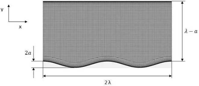
computational domain was two-dimensional in our case as is shown in Figure 1. It consists of a channel which is unbounded in the streamwise direction. The lower wall has two waves with sinusoidal shape and a mean position at the y=0. The flat upper wall is located at y=λ. The location of the wavy wall is given by
ݕ ൌ ܽ ʹߨݔ
ߣ ǡ (1)
where ܽ is the amplitude of the wave and λ is the wavelength. The Reynolds number based on bulk velocity Ub and mean height of the channel h=λ was set Re=hUb/ν=6760.
The wave amplitude to the wavelength ratio equals 0.05.
Figure 1: Computational domain and grid system.
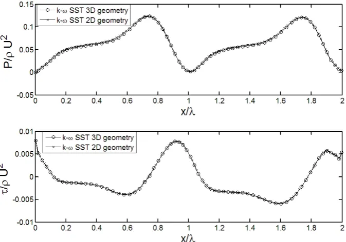
Because the flow is assumed to be homogeneous in the spanwise direction, periodic boundary conditions have been used in DNS simulations. However, in our case we have used only two-dimensional geometry. From the comparison with results for three- dimensional geometry, see Figure 2, it follows that this simplification is acceptable at least for values of wall shear stress and pressure forces. Thus, the periodic boundary conditions are assigned and the constant mass flow rate is adjusted in the streamwise direction.
3. NUMERICAL METHOD
All simulation in the present study used Nx=114 and Ny=76÷80 grid points in the
streamwise and wall-normal direction, respectively, depending on the x location. Uniform grid was used in the streamwise direction, while in the wall-normal direction finer grid was adjusted in the near wall region to better resolve the boundary layers. The y+ values on the whole wavy wall have been less than 0.2, therefore the boundary layer can be directly resolved.
of flow separation. We used the standard Wilcox’s k-ω [8], k-ω SST of Menter [9] and finally k-ε V2F [10] RANS equations model.
Figure 2: Comparison of pressure and wall shear stress distribution at wavy wall for 2D and 3D geometry by using k-ω SST turbulence model.
4. R
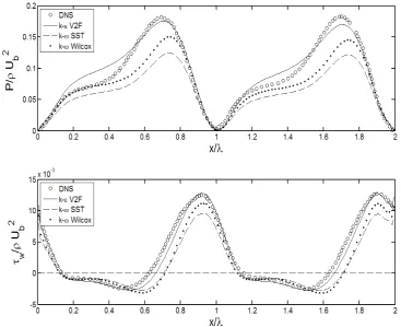
ESULTSThe normalized mean pressure and wall shear stress distributions along the wavy wall are plotted in Figure 3. Note that the pressures were obtained by subtracting of the linear pressure drop (-Pxx). Thus, pressures distribution does not decrease along the wavy
surface in x-direction as would in the real case.
By following the definition of the separation and reattachment points as points where wall shear stress equals zero, the locations of separation and reattachment point are found at x/λ=0.14 and x/λ=0.62, respectively, according DNS results from [7].
x/λ location of DNS k-ε V2F k-ω SST Wilcox’s k-ω
separation point 0.14 0.14 0.13 0.13
reattachment point 0.62 0.66 0.71 0.71
Table 1: The x/λ location of separation and reattachmnet points predicted by selected models.
extreme values of pressure and wall shear stress by this model gives relatively good and very good results, respectively. This is in good agreement with the fact, that this model is designed to capture the near-wall turbulence effects more accurately, which is crucial for prediction of skin friction and flow separation.
The both k-ω models prediction of pressure and wall shear stress distribution are quite similar. They differ most in predicting of the maximum values. The Figure 3 shows that the k-ω SST model underestimates most of all selected models the two observed variables.
Figure 3: Comparison of pressure and wall shear stress distributions at wavy wall normalized by ρUb2 and computed by using of selected RANS models.
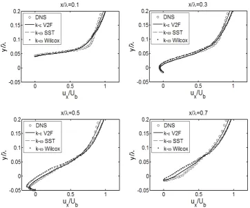
The streamwise velocity profiles in near-wall region resolved by the selected models and normalized by bulk velocity Ub are plotted in figure 3 for x/λ=0.1, 0.3, 0.5 and 0.7. As is
shown, the profiles computed using selected RANS models are quite similar and agree well with DNS results at x/λ=0.1 and x/λ=0.3. Only the sharp curvature of the turbulence profile around y/λ=0.075 at x/λ=0.1 is not well captured. However, the profiles differ more from DNS results at other two locations x/λ=0.5 and x/λ=0.7. The two k-ω models give still very similar results, but these does not fit very well DNS data. However, the k-ε V2F model gives quite good agreement with direct numerical simulation as well as in the previous locations. These facts correspond with the flow separation area, which can be seen from wall shear stress depicted in Figure 3.
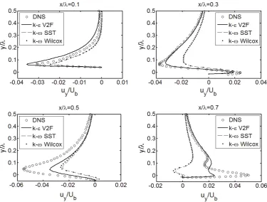
previous figure. It can be seen that the greatest difference between DNS data and results of both k-ω RANS models occurs for x/λ=0.7, because the reattachment point is located around x/λ=0.71 for these models. The profiles computed by the k-ε V2F model are the best from the selected models again. The results are quite good in comparison with DNS data, however the difference become greater near the reattachment point.
5. CONCLUSIONS
The present study has presented the comparison of the selected turbulence models (i.e. Wilcox’s k-ω, k-ω SST and k-ε V2F) in using for simulation of turbulent flow over the wavy surface. The pressure and wall shear stress distributions and the velocity profiles were used to compare results of the RANS equations models with attitude of DNS.
It has been shown that all of RANS models predict the location of separation point quite well, but they all overpredict the location of reattachment point. The results of both k-ω models are almost the same and do not fit the DNS results very well especially near the flow separation. However, from pressure and wall shear stress distributions as well as from velocity profiles has been shown that the k-ε V2F model gives the best results in comparison with DNS attitude. This conclusion is consistent with expectation regarding to field of use of the selected models.
Figure 5: Wall-normal velocity profiles at difference streamwise locations: x/λ=0.1, 0.3, 0.5 and 0.7.
6. A
CKNOWLEDGEMENTThe article was supported from GA ČR project GA101/08/0096 and from FSI-S-11-6.
7. REFERENCES
[1] Zilker D.P., Cook G.W. and Hanratty T.J.: Influence of the amplitude of a solid wavy wall on a turbulent flow. Part 1. Non-separated flows, J. Fluid Mech., 82, 1977, 29-51
[2] Zilker D.P. and Hanratty T.J.: Influence of the amplitude of a solid wavy wall on a turbulent flow. Part 2. Separated flows, J. Fluid Mech., 90, 1979, 257-271 [3] Hudson J.D.: The effect of a wavy boundary on turbulent flow, Ph.D. Thesis,
University of Illinois, Urbana, IL, 1993
[4] Hudson J.D., Dykhno L. and Hanratty T.J.: Turbulence production in flow over a wavy wall, Exper. Fluids, 20, 1996, 257
[5] Maass C. and Schumann U.: Direct numerical simulation of separated turbulent flow over wavy boundary, In: Hirschel E.H. (Ed.): Flow simulation with high performance computers, Notes on numerical fluid mechanics, 52, 1996, 227-241
[7] Yoon H.S., El-Samni O.A., Huynh A.T., Chun H.H., Kim H.J., Pham A.H. and Park I.R.: Effect of wave amplitude on turbulent flow in a wavy channel by direct numerical simulation, Ocean Engineering, 36, 2009, 697-707
[8] Wilcox D.C.: Turbulence Modeling for CFD, 2nd edition, DCW Industries, Inc., 1998
[9] Menter F.R.: Two-equation eddy-viscosity turbulence modeling for engineering applications, AIAA Journal, 32 (8), 1994, 1598-1605.