Article
1
Modeling Natural Gas Compressibility Factor Using
2
a Hybrid Group Method of Data Handling
3
Abdolhossein Hemmati-Sarapardeh 1, Sassan Hajirezaie 2, Mohamad Reza Soltanian 3,
4
Amir Mosavi 4,5, and Shahaboddin Shamshirband 6,7,*
5
1 Department of Petroleum Engineering, Shahid Bahonar University of Kerman, Kerman, Iran;
6
7
2 Department of Civil and Environmental Engineering, Princeton University, Princeton, United States;
8
9
3 Department of Geology, University of Cincinnati, Cincinnati, OH 45221, United States; [email protected]
10
4 Faculty of Health, Queensland University of Technology, Brisbane QLD 4059, Australia;
11
12
5 School of the Built Environment, Oxford Brookes University, Oxford OX3 0BP, UK;
13
14
6 Department Department for Management of Science and Technology Development, Ton Duc Thang
15
University, Ho Chi Minh City, Vietnam
16
7 Faculty of Information Technology, Ton Duc Thang University, Ho Chi Minh City, Vietnam
17
* Correspondence: [email protected]
18
19
Abstract: A Natural gas is increasingly being sought after as a vital source of energy, given that its
20
production is very cheap and does not cause the same environmental harms that other resources,
21
such as coal combustion, do. Understanding and characterizing the behavior of natural gas is
22
essential in hydrocarbon reservoir engineering, natural gas transport, and process. Natural gas
23
compressibility factor, as a critical parameter, defines the compression and expansion characteristics
24
of natural gas under different conditions. In this study, a simple second-order polynomial model
25
based on the group method of data handling (GMDH) is presented to determine the compressibility
26
factor of different natural gases at different conditions, using corresponding state principles. The
27
accuracy of the model evaluated through graphical and statistical analyses. The results show that
28
the model is capable of predicting natural gas compressibility with an average absolute error of only
29
2.88%, a root means square of 0.03, and a regression coefficient of 0.92. The performance of the
30
developed model compared to widely known, previously published equations of state (EOSs) and
31
correlations, and the precision of the results demonstrates its superiority over all other correlations
32
and EOSs.
33
Keywords: Natural gas; gas compressibility factor; group method of data handling (GMDH); big
34
data; Equation of state; Correlation
35
36
1. Introduction
37
The increasing demand for oil and coal as energy and the technological and environmental
38
concerns associated with its production and consumption have drawn attention toward natural gas.
39
The natural gas consumption generates less pollutants and greenhouse gases [1, 2]. Understanding
40
the behavior of natural gas is important to all reservoir and chemical engineering calculations that
41
deal with gas as one of the main phases. Among the parameters of evaluating the behavior of natural
42
gas, the gas compressibility factor is essential for determining the natural gas’s phase behavior. Gas
43
compressibility represents the proportion of volume a given amount of gas at a specific pressure and
44
temperature to the ideal volume of it at the common conditions. Gas compressibility makes the
45
difference between ideal gas and real gas. The following relationship is generally used to calculate
46
gas compressibility:
47
(1)
48
Where R represents the universal gas constant and z is the gas compressibility factor. Vreal (V)
49
and Videal denote real and ideal gas volumes, respectively. T and P and n represent the gas
50
temperature, pressure, and some moles, respectively.
51
At low pressure and temperature conditions, gas molecules have fewer interactions and
52
collisions, and behavior can be considered ideal. However, at high temperature and pressure, the
53
collisions between the molecules become critical and need to be taken into account when making
54
predictions for gas expansion or contraction [2, 3].
55
There are various techniques to measure the compressibility factor. One main way is by
56
performing compression-expansion experiments. Overall, the experimental measurement of
57
compressibility factor appeared to be an accurate approach compared to all other approaches.
58
However, they are generally slow, cumbersome, and costly. Also, it is reported not feasible to conduct
59
an experiment for every single condition considering various pressure and temperature at which the
60
compressibility is needed. Using equations of state (EOS) is another approach to determine the
61
compressibility factor. When utilizing EOS, the reservoir characteristics are being employed.
62
Generally, these equations come from the following form when the gas compressibility factor is the
63
target PVT parameter:
64
(2)
65
where a, b, and c represent the empirical constants of composition functions for temperature,
66
pressure, and gas. Furthermore, Z denotes the gas compressibility factor. Even though these
67
equations are advantages and their implementation can facilitate the measurement of other gas
68
properties such as enthalpy, entropy, and Gibbs free energy, they are usually implicit higher-order
69
equations that require intense computations. Besides the complex computations, the binary
70
interaction coefficients used in some EOS’s need to be measured by conducting experiments that may
71
not be practical. Further, it has been shown that these equations are not suitable for predicting
72
hydrocarbon gas properties [4].
73
Empirical correlations are another source of determining gas compressibility factor, which is
74
easy and fast to use but is generally associated with erroneous predictions [5-7]. A minor estimation
75
error in compressibility factor of correlations would lead to false prediction of formation, density and
76
the amount of gas. Therefore, development of fast, user-friendly, and accurate models to predict the
77
compressibility factor is critical.
78
Several researchers have attempted to develop methods to estimate the compressibility factor.
79
For instance, Katz and Standing [8] developed a graphical approach of the basis of pseudo-reduced.
80
Van der Waals [9] was one of the pioneers of EOS methods by taking into account the intramolecular
81
forces and volume of molecules. Using Van der Waals EOS for determining gas compressibility factor
82
leads higher accuracy compared to the empirical approach introduced by Katz and Standing. Other
83
authors who contributed to the development of reliable EOS’s are Peng–Robinson [10], Lawal–Lake–
84
Silberberg [11], Patel–Teja [12], and Soave–Redlich–Kwong [13].
85
A general expression for the PVT relationship of fluids has the following form [2]:
86
(3)
87
An expression for gas compressibility factor can be written by rewriting the above equation and
88
implementing the equation for gas compressibility factor as follows:
89
(4)
90
Where A, B U, and W are dimensionless parameters that can be determined from the current
91
In order to develop faster methods, several authors have developed correlations that can be
93
explicitly used to address the problem. In 1973, Hall and Yarborough [14] transformed the graphical
94
chart of Katz and Standing into a relatively simple correlation by fitting their correlation to the chart
95
and determining the correlation coefficients. Brill and Beggs [15] also employed Katz and Standing
96
chart and developed a correlation to estimate gas compressibility factor. Dranchuk [16] used an EOS
97
developed by Benedict–Webb–Rubin [17] and proposed a gas compressibility correlation in 1974.
98
Abu-Kassem joined Dranchuk in 1975 to develop an analytical equation for reduced gas density that
99
can be efficiently utilized to determine gas compressibility factor [18]. In 1975, Gopal collected
100
multiple correlations for the gas compressibility factor at various conditions [19]. Kumar [6]
101
introduced a novel model for gas compressibility factor to be used by Shell. In 2010, Heidaryan et al.
102
used multiple regression analysis [20], and in the same year, Azizi employed genetic programming
103
[21]. A comprehensive study of the mentioned methods was conducted by Sanjari and Lay [22] in
104
which the performance of the methods mentioned above have been investigated.
105
Recently, the usage of intelligent models in the oil and gas industry has attracted much attention.
106
These models have been used to determine, oil and gas thermodynamic properties, reservoir
107
formation properties and miscibility conditions required for gas injection processes [23-32]. These
108
models take both input and output values to get trained and later can make predictions. Even though
109
the original, intelligent models were considered black box models, there have been numerous
110
modifications to these models to make them transparent and usable methods, and their performance
111
has significantly improved over the past few years. Intelligent models have been used in many
112
reservoir engineering calculations. There are also some intelligent models that were developed
113
specifically for predicting natural gas properties [23-25]. We have already developed two intelligent
114
models for predicting natural gas compressibility factor using the same data bank of this study [1, 2].
115
However, they are a black box, and their usage generally needs software.
116
In this study, a novel supervised approach of GMDH proposed as a robust model to estimate
117
the compressibility factor. To do this, a comprehensive data bank of compressibility factor at wide
118
ranges of temperature, pressure, and composition was used. Several statistical quality measures and
119
graphical techniques were used to assess and evaluate the performance of the proposed model. These
120
statistical and graphical methods include root mean square error (RMSE), average absolute percent
121
error (AAPRE), regression coefficient (R2), average percentage relative error (APRE), crossplot, and
122
error distribution curves. Additionally, the performance of previously published well-known
123
correlations and EOSs was investigated and compared to the proposed model. references.
124
2. Data Acquisition
125
The reliability of any intelligent model is dependent on the data bank that has been utilized
126
during the training and testing stages of model development. Here, various range of pressure,
127
temperature, and gas composition conditions were used to ensure the development of a valid model
128
that can determine the gas compressibility factor. Two dimensionless parameters of pseudo-reduced
129
for temperature and pressure are defined to be used in the developed model for predicting gas
130
compressibility. These parameters are calculated from the current pressure and temperature, and the
131
pseudo critical pressure and temperature described as:
132
(5)
133
where Ppc and Tpc represent the pseudo critical pressure and temperature, respectively. In
134
addition, Ppr and Tpr are the pseudo-reduced pressure and temperature.
135
For a gas with multiple components, Ppc and Tpc are calculated from the critical temperature and
136
pressure of the individual components as follows:
137
𝑃 = ∑ 𝑦 𝑃 (6)
138
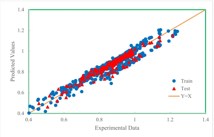
𝑇 = ∑ 𝑦 𝑇 (7)
In these equations, Tci and Pci stand for the critical temperature and pressure of component i, and
140
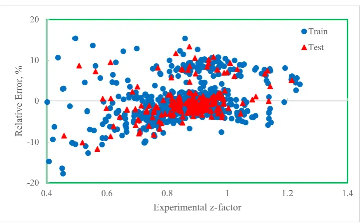
yi describes the mole fraction of the component i.
141
The data sets in this article were collected from various literature sources [17, 33-38]. Further the
142
Table 1 represents the statistical details of the data bank used. As the table demonstrates, the
143
pressures, temperatures, and compositions comprise a comprehensive range, ensuring that the
144
developed model based on this data set would be a reliable predictor for various types of natural
145
gases at different conditions.
146
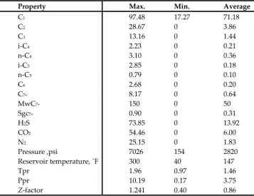
147
Table 1: The statistical parameters for the data used for z-factor modeling
148
Property Max. Min. Average
C1 97.48 17.27 71.18
C2 28.67 0 3.86
C3 13.16 0 1.44
i-C4 2.23 0 0.21
n-C4 3.10 0 0.36
i-C5 2.85 0 0.18
n-C5 0.79 0 0.10
C6 2.68 0 0.20
C7+ 8.17 0 0.64
MwC7+ 150 0 50
Sgc7+ 0.90 0 0.31
H2S 73.85 0 13.92
CO2 54.46 0 6.00
N2 25.15 0 1.83
Pressure ,psi 7026 154 2820
Reservoir temperature, ˚F 300 40 147
Tpr 1.96 0.97 1.46
Ppr 10.19 0.17 3.75
Z-factor 1.241 0.40 0.86
149
3. Evaluating the model performance
150
There are multiple statistical parameters that are employed to assess the performance of a model.
151
The parameters that were used in this work include APRE, AAPRE, RMSE, and R2. A simple
152
presentation of the mentioned parameters is presented here:
153
1. APRE (Er%):
154
==
ni i r
n
E
E
1
1
(8)
where Ei stands for the relative variation of predicted value from an experimental value
155
expressed as Percentage Relative Error:
156
( )
( )
i
n
O
O
O
E
i100
1
,
2
,
3
,...,
exp rep./pred exp
=
×
−
=
(9) 2. AAPRE:157
==
n i i an
E
E
1|
|
1
(10)3. RMSE:
158
(
)
=−
=
n i i iO
O
n
RMSE
1 2 rep./pred exp1
(11)(
)
(
)
= =
−
−
−
=
ni n
i i
O
O
O
O
R
1
2 rep./pred i 1
2 rep./pred i exp 2
1
(12)
In these formulas,
O
is the mean value of experimental data output.160
Another approach to evaluate the performance of a model and compare it with other models is
161
the usage of graphical error analysis. The graphical approaches used in this study are cross-plot,
162
frequency vs. absolute relative error, error distribution and trend analysis curves. Crossplots are
163
utilized to assess the performance of a model in which the estimated data by the model are plotted
164
against the experimental values, and one can observe the accuracy of the model depending on how
165
close the trend is to a unit-slope line that crosses the origin. Further, the cumulative frequency of data
166
points against the absolute relative error is plotted to quantify the number of data points that can be
167
accurately predicted by the model. Besides, the error distribution curve was plotted to evaluate the
168
error trend of the model when an independent variable is increased. The proximity of data points
169
to the zero-error line tests the precision of that model. Finally, a trend analysis is performed to
170
investigate whether or not the developed model can accurately estimate the trend of gas
171
compressibility factor at different pressures.
172
173
4. Model Development
174
GMDH, every two independent parameters are coupled with a quadratic polynomial expression
175
and form 𝐌𝟐 new variables as follows:
176
(14)
177
And the new matrix can be represented by the new variables as follows:
178
(15)
179
In the next step, the least square method is utilized to reduce the difference between the actual data
180
and the model predictions as presented below:
181
(16)
182
In this equation, the quantity of data points in the training set is shown by Nt. In the next step, the
183
general matrix is written as follows:
184
(17)
185
Writing the general matrix in the above form helps with offering a general formulation to
186
determine the unknown quadratic polynomial coefficients as shown below:
187
(18)
188
In the later stage, the data set is divided into subsets of testing and training, the model coefficients
189
are obtained during the training stage, and the testing set is utilized to determine the best
190
(19)
192
The combined variables will be stored if this criterion is met, otherwise the algorithm eliminates
193
this combination of two variables and the iteration will continue. More information about this
194
modeling approach can be found in our previous work [46].
195
5. Results
196
AThe GMDH has been successfully implemented as an evolutionary intelligent model to predict
197
the natural gas’s compressibility. The inputs of the model were gas composition, pressure, and
198
temperature as shown in Table 1. In addition to C1-C6 and C7+ components, H2S, CO2, and N2 gases
199
were considered as the components. The pressure and temperature values are used to calculate the
200
pseudo-reduced pressure and temperature as discussed previously. During the data acquisition
201
stage, a wide range of input parameters was considered as shown in Table 1. The pressure ranges
202
from 154 to 7026 Psia, reservoir temperature ranges from 40 to 300 0 F, and the compressibility factor
203
values cover a wide range of 0.4 to 1.24. The distribution of input and output data is illustrated in
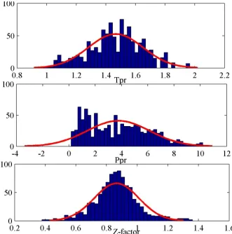
204
Figure 1. In addition to the data distribution, normal distribution curves were plotted in this figure.
205
Pseudo reduced pressure and temperature were the chosen parameters for this figure due to their
206
impact on any reservoir fluid properties. As can be seen, all three data sets follow a relatively normal
207
shape, especially the gas compressibility factor data. The mean values for the pseudo-reduced
208
temperature, pseudo-reduced pressure, and gas compressibility factor are 1.5, 3.9 and 0.9,
209
respectively. The bin size in all cases is 40. A schematic flowchart of the model is illustrated in Figure
210
2. In order to assess the accuracy of the developed model, various statistical and graphical methods
211
such as average absolute relative error and error distribution curve were employed as will be
212
discussed in this section.
213
214
215
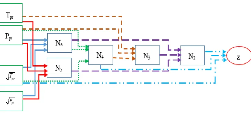
217
218
Fig. 2: A schematic flowchart of the proposed GMDH for predicting z-factor
219
220
221
After optimizing the model, the genome and nodal expressions were obtained as follows:
222
223
2 2 4 4 2 pr pr2
T
+
0.434222T
-
1.02209N
+
0.397836N
+
2.58207N
1.09959N
-0.268213
-
=
z
(20)224
pr pr pr pr pr pr pr6
=
2.28818
+
1.46235P
-
1.05874P
T
+
3.50204
T
P
-
0.667833T
-
4.84879
P
N
(21)225
pr pr 2 pr pr pr pr pr5
=
1.88105
-
0.466011T
P
+
1.5661T
P
-
0.265557T
+
0.863307P
-
2.90311
P
N
(22)226
6 pr pr 6 2 pr 6 pr4
=
-
2.14451
-
0.0929261P
N
+
0.0120013P
-
4.51872N
T
+
1.89131T
+
5.85344N
N
(23)227
2 4 4 2 pr pr 2 pr3
=
-
0.461086
+
0.0344126T
-
0.048752P
+
0.00674994
P
+
2.4872N
-
1.11543N
N
(24)228
3 3 6 6 3 5 52
=
-
0.182453
-
17.0122N
+
18.4918
N
N
+
17.1725N
-
18.6856N
N
+
1.22045N
N
(25)
229
230
where Tpr and Ppr represent the pseudo-reduced temperature and pressure, respectively, and N2
-231
N6 represent the virtual variables or nodes of the model. It should be noted that the equations are
232
second order polynomials that can be easily used to estimate the gas compressibility factor. As can
233
be seen in the first equation, gas compressibility factor can be calculated by having the pseudo-
234
reduced temperature, and the virtual parameters N2 and N4 and. N4 can be calculated by knowing
235
pseudo-reduced pressure and by calculating the virtual parameter N6. N6 is a simple function of
236
temperature and pseudo-reduced pressure and can be directly calculated. In order to calculate N2,
237
the virtual parameters N3 and N5 are needed in addition to N6. N3 can be calculated after calculating
238
the virtual parameter N4. Finally, N5 can be directly calculated similarly to N6 by having
pseudo-239
reduced pressure and temperature. Statistical quality measures and graphical techniques were
240
applied to assess the performance of the developed model, as well as to compare the model with the
241
results of five of the well-known EOSs namely van der-Waals [47] EOS, Lawal-Lake-Silberberg [48]
242
EOS, Peng-Robinson [10] EOS, Soave-Redlich-Kwong [13] EOS, and Patel-Teja [12] EOS as well as ten
243
empirical correlations namely, Dranchuk-Purvis-Robinson [49], Dranchuk-Abou-Kassem [18],
244
Beggs-Brill [50], Shell Oil Company [6], Gopal [51], Hall-Yarborough [14], Sanjari and Lay [22],
245
Heidaryan et al. [20], Azizi et al. [21], and Kamari et al. [52]. Table 2 presents the results of a statistical
246
assessment of the GMDH model and previously published correlations and EOSs. As can be observed
247
in this table, the developed model demonstrates the most accurate performance compared to other
248
regression coefficient. The Hall Yarborough correlation was found to be the next most accurate model
250
followed by the Patel-Teja EOS model based on the statistical information presented in this table.
251
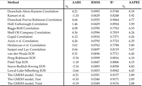
252
Table 2: Statistical error analyses for the correlations, EOSs, and the GMDH model
253
Method AARE %
RMSE R² AAPRE
%
Dranchuk-Abou-Kassem Correlation 4.21 0.0992 0.5748 8.18
Kamari et al. -1.10 0.0629 0.8248 5.92
Dranchuk-Purvis-Robinson Correlation 4.66 0.0555 0.9064 4.77
Hall-Yarborough Correlation 1.46 0.0429 0.8924 3.59
Beggs-Brill Correlation 4.08 0.0785 0.7763 6.53
Shell Oil Company Correlation 4.36 0.0596 0.7819 6.24
Gopal Correlation 6.12 0.0910 0.7371 6.26
Azizi et al. Correlation 4.26 0.0792 0.7723 6.25
Heidaryan et al. Correlation 3.61 0.0762 0.7788 5.80
Sanjari and Lay Correlation 0.66 0.0697 0.8119 5.67
van der-Waals EOS 0.31 0.0696 0.7711 6.42
Peng-Robinson EOS -5.34 0.0599 0.8916 6.10
Patel-Teja EOS -1.18 0.0447 0.8806 4.15
Soave-Redlich-Kwong EOS -3.14 0.0493 0.8938 4.82
Lawal-Lake-Silberberg EOS -2.66 0.0453 0.8942 4.43
The GMDH model, Train -0.21 0.0351 0.9177 2.89
The GMDH model, Test -0.10 0.0340 0.9171 2.85
The GMDH model, Total -0.19 0.0349 0.9176 2.88
254
Noticing the APRE and AAPRE values of the models in this study reveals that, while the APRE
255
value of some of the models is not smaller than those of others, their AAPRE is. The definition of
256
APRE can be used to explain this observation. As a matter of fact, APRE (Average Percentage Relative
257
Error) is a relative value and should not be used by itself to approve or reject a model. For instance,
258
an APRE value close to zero would be obtained if half of the data points are overestimated by a model
259
and the remaining half are underestimated, which would in return present a false assessment of the
260
model performance. On the other hand, if most of the data points are estimated accurately by a model
261
and the remaining few data points are either underestimated or overestimated, a positive or negative
262
APRE value would be obtained, respectively, which again cannot testify the model performance. As
263
an example, Van der Waals model has a much smaller APRE value than that of
Dranchuk-Purvis-264
Robinson. However, it is considered to be a less accurate model than the latter one
265
Another way to illustrate the performance of the models and to compare them more
266
comprehensively is by using graphical analyses. Several graphical analyses were employed in this
267
work to evaluate the performance of the most popular models from both quantity and quality
268
standpoints. Figure 3 presents the cross-plot of the developed model in which the calculated data is
269
plotted against the measured data for both testing and training sets. The location of the majority of
270
the data points on the y=x line supports the accurate predictions of the developed GMDH model.
271
This is true for both of the training and testing data sets. The error distribution of the model is shown
272
in Figure 4. As the figure shows, most of the data points are near the zero percent error line. This
273
indicates that the GMDH model does not have a systematic error trend as the gas compressibility
274
factor increases (most of the previously published models suffer from an error trend). The figure
275
indicates that the error of the testing set is smaller than the training set. The distribution of the relative
276
error of predictions is plotted in Figure 5. In addition to the distribution of data points, the normal
277
distribution is plotted indicated by the red line. The figure indicates that the relative error of
278
predictions accurately follows the normal distribution and that most of the data points (predictions)
279
have a relative error close to zero demonstrating the accuracy of the mode in predicting gas
280
graphical demonstration of the performance of the models. Further, these figures indicate that models
282
with a smaller RMSE do not necessarily have a smaller average absolute percent relative error. This
283
means that when performing statistical analyses, care should be taken to avoid the misinterpretation
284
of the results by focusing on only one statistical parameter.
285
286
287
Fig. 3: Crossplot of the predicted z-factors versus experimental data
288
289
0.4 0.6 0.8 1 1.2 1.4
0.4 0.6 0.8 1 1.2 1.4
Pred
icted
Valu
es
Experimental Data
290
291
292
293
Fig. 4: Error distribution curve of the proposed GMDH model versus experimental z-factor
294
295
296
Fig. 5: Distribution of relative error of the proposed GMDH model
297
298
-20 -10 0 10 20
0.4 0.6 0.8 1 1.2 1.4
Relativ
e Erro
r,
%
Experimental z-factor
299
Fig. 6: RMSE of the existing correlations, EOSs, and GMDH models for predicting z-factor
300
301
302
303
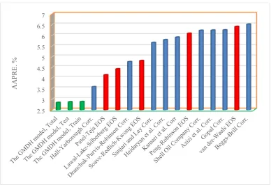
Fig. 7: Average absolute percent relative error of the existing correlations, EOSs, and GMDH
304
models for predicting z-factor
305
306
307
As can be seen in Figure 7, Beggs-Brill, Van der Waals, Gopal, Azizi, and Shell Oil Company
308
models have the highest AAPRE values meaning that their predictions are less accurate than other
309
models. It can be observed that the proposed model in this work is distinctly superior to the
310
previously published models by an AAPRE of only 2.89%, 2.85%, and 2.88% for the training, testing
311
and total data sets, respectively. A better vision of the superiority of the suggested model can be
312
observed in Figure 6 in which the developed model has a much smaller RMSE value than all of the
313
published models.
314
315
0.03 0.04 0.05 0.06 0.07 0.08 0.09 0.1
RMSE
2.5 3 3.5 4 4.5 5 5.5 6 6.5 7
AAPRE.
316
Fig 8. Cumulative frequency versus absolute relative error for existing models as well as the
317
proposed GMDH model for predicting gas compressibility factor
318
319
320
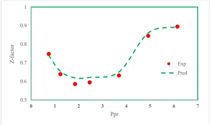
321
Fig. 9: Variation of z-factor as a function of Ppr at Tpr=1.19 for a gas sample
322
323
In order to compare the accuracy of the developed GMDH model with the previously published
324
correlations, cumulative frequency plots of the models are illustrated in Figure 8. This figure helps to
325
achieve a better quantitative evaluation of the developed model when compared to the previously
326
published models. This figure shows that the GMDH model can predict nearly 52% of the data with
327
an absolute relative error of 2%. More importantly, the model can predict 75% of the data points with
328
an absolute relative error of only 4%. It can be observed that the model estimates the gas
329
compressibility factor with the smallest absolute relative error for any number of data points included
330
in the predictions. This verifies the consistency of the developed GMDH model in accurately
331
estimating gas compressibility factor within a wide range of reservoir conditions. The figure also
332
shows that Hall-Yarborough correlation is the next accurate model that can estimate gas
333
compressibility factor with small error values when any number of data points are considered.
334
Another important finding from this figure is the comparison between Lawal-lake-Silberberg EOS
335
model and Dranchuk-Purvis-Robinson correlation. While Lawal-lake-Silberberg EOS is more
336
0 0.1 0.2 0.3 0.4 0.5 0.6 0.7 0.8 0.9 1
0 2 4 6 8
Cumulative
F
requency
Absolute Relative Error, %
Hall-Yarborough Corr.
Lawal-lake-Silberberg EOS
Dranchuk-Purvis-Robinson Corr. Soave-Redlich-Kwong EOS
Patel-Teja EOS
GMDH
ARE=2%
0.5 0.6 0.7 0.8 0.9 1
0 1 2 3 4 5 6 7
Z-factor
Ppr
accurate in estimating gas compressibility factor for up to 50% of the data points,
Dranchuk-Purvis-337
Robinson correlation becomes the superior model when more than 50% of the data points are
338
included. This trend changes again when 80% or more of the data points are included.
339
Finally, the predicted compressibility values by the GMDH model were plotted in Figure 9
340
against the experimental data at different reduced pressure values and constant
pseudo-341
reduced temperature of 0.7 to confirm the capability of the developed model in accurately estimating
342
natural gas compressibility factor at different conditions. The experimental trend in this figure
343
indicates that by increasing the pressure, gas compressibility factor first decreases and then increases.
344
This trend has been accurately estimated by the developed GMDH model as shown by the dashed
345
line in the same figure.
346
5. Conclusions
347
In this work, GMDH was used to predict the compressibility factor of natural gas. The results
348
showed that the developed model’s performance is consistently more accurate than the previously
349
published well-known correlations at different temperature and pressure conditions. This was
350
confirmed by measuring the root mean square, average absolute percent relative error, and
351
regression coefficient to be 0.03, 2.88%, and 0.92, respectively. The Hall Yarborough correlation was
352
determined as the second most accurate correlation for estimating the natural gas compressibility
353
factor. In addition, the error distribution curve analysis indicated that the presented model in this
354
study does not have an error trend when predicting very low and very high compressibility factor
355
values. The experimental trend of gas compressibility factor showed that by increasing the pressure,
356
the Z-factor first decreases and then increases. This trend was perfectly shown by the developed
357
GMDH model in this work.
358
The results of this study show that most of the previously published correlations have been
359
developed based on limited data sets and are only able to estimate the compressibility factor within
360
limited ranges of pressure and temperature conditions. While, the proposed GMDH model can
361
accurately predict the natural different gas compressibility factor at low and high temperature and
362
pressure conditions.
363
Conflicts of Interest: Authors declare conflicts of interest or state.
364
References
365
1. Kamari, A., et al., Prediction of sour gas compressibility factor using an intelligent approach. Fuel processing
366
technology, 2013. 116: p. 209-216.
367
2. Shateri, M., et al., Application of Wilcoxon generalized radial basis function network for prediction of natural gas
368
compressibility factor. Journal of the Taiwan Institute of Chemical Engineers, 2015. 50: p. 131-141.
369
3. Firoozabadi, A., Thermodynamics of hydrocarbon reservoirs. 1999: McGraw-Hill New York.
370
4. Elsharkawy, A.M., Efficient methods for calculations of compressibility, density and viscosity of natural gases. Fluid
371
Phase Equilibria, 2004. 218(1): p. 1-13.
372
5. Kamyab, M., et al., Using artificial neural networks to estimate the z-factor for natural hydrocarbon gases. Journal
373
of Petroleum Science and Engineering, 2010. 73(3-4): p. 248-257.
374
6. Kumar, N., Compressibility factors for natural and sour reservoir gases by correlations and cubic equations of state.
375
2004, Texas Tech University.
376
7. Sanjari, E. and E.N. Lay, Estimation of natural gas compressibility factors using artificial neural network approach.
377
Journal of Natural Gas Science and Engineering, 2012. 9: p. 220-226.
378
9. Van Der Waals, J.D. and J.S. Rowlinson, On the continuity of the gaseous and liquid states. 2004: Courier
380
Corporation.
381
10. Peng, D.-Y. and D.B. Robinson, A new two-constant equation of state. Industrial & Engineering Chemistry
382
Fundamentals, 1976. 15(1): p. 59-64.
383
11. Lawal, A., Application of the Lawal-Lake-Silberberg equation-of-state to thermodynamic and transport properties of
384
fluid and fluid mixtures, in Technical Report TR-4-99. 1999, Department of Petroleum Engineering, Texas Tech
385
University Lubbock.
386
12. Patel, N.C. and A.S. Teja, A new cubic equation of state for fluids and fluid mixtures. Chemical Engineering
387
Science, 1982. 37(3): p. 463-473.
388
13. Soave, G., Equilibrium constants from a modified Redlich-Kwong equation of state. Chemical engineering science,
389
1972. 27(6): p. 1197-1203.
390
14. Hall, K.R. and L. Yarborough, A new equation of state for Z-factor calculations. Oil Gas J, 1973. 71(25): p. 82.
391
15. Beggs, D.H. and J.P. Brill, A study of two-phase flow in inclined pipes. Journal of Petroleum technology, 1973.
392
25(05): p. 607-617.
393
16. Dranchuk, P., R. Purvis, and D. Robinson. Computer calculation of natural gas compressibility factors using the
394
Standing and Katz correlation. in Annual Technical Meeting. 1973. Petroleum Society of Canada.
395
17. Simon, R. and J.E. Briggs, Application of Benedict-Webb-Rubin equation of state to hydrogen sulfide-hydrocarbon
396
mixtures. AIChE Journal, 1964. 10(4): p. 548-550.
397
18. Dranchuk, P. and H. Abou-Kassem, Calculation of Z factors for natural gases using equations of state. Journal of
398
Canadian Petroleum Technology, 1975. 14(03).
399
19. Gopal, V., Gas z-factor equations developed for computer. Oil and Gas Journal, 1977. 75(8): p. 8-13.
400
20. Heidaryan, E., J. Moghadasi, and M. Rahimi, New correlations to predict natural gas viscosity and compressibility
401
factor. Journal of Petroleum Science and Engineering, 2010. 73(1-2): p. 67-72.
402
21. Azizi, N., R. Behbahani, and M. Isazadeh, An efficient correlation for calculating compressibility factor of natural
403
gases. Journal of Natural Gas Chemistry, 2010. 19(6): p. 642-645.
404
22. Sanjari, E. and E.N. Lay, An accurate empirical correlation for predicting natural gas compressibility factors.
405
Journal of Natural Gas Chemistry, 2012. 21(2): p. 184-188.
406
23. Hajirezaie, S., et al., A smooth model for the estimation of gas/vapor viscosity of hydrocarbon fluids. Journal of
407
Natural Gas Science and Engineering, 2015. 26: p. 1452-1459.
408
24. Dargahi-Zarandi, A., et al., Modeling gas/vapor viscosity of hydrocarbon fluids using a hybrid GMDH-type neural
409
network system. Journal of Molecular Liquids, 2017. 236: p. 162-171.
410
25. Hajirezaie, S., et al., Development of a robust model for prediction of under-saturated reservoir oil viscosity. Journal
411
of Molecular Liquids, 2017. 229: p. 89-97.
412
26. Hemmati-Sarapardeh, A., et al., On the evaluation of density of ionic liquid binary mixtures: modeling and data
413
assessment. Journal of Molecular Liquids, 2016. 222: p. 745-751.
414
27. Kamari, A., A. Safiri, and A.H. Mohammadi, Compositional model for estimating asphaltene precipitation
415
28. Rostami, A., et al., New empirical correlations for determination of Minimum Miscibility Pressure (MMP) during
417
N2-contaminated lean gas flooding. Journal of the Taiwan Institute of Chemical Engineers, 2018. 91: p. 369-382.
418
29. Kamari, A., et al., Characterizing the CO2-brine interfacial tension (IFT) using robust modeling approaches: A
419
comparative study. Journal of Molecular Liquids, 2017. 246: p. 32-38.
420
30. Hajirezaie, S., et al., Numerical simulation of mineral precipitation in hydrocarbon reservoirs and wellbores. Fuel,
421
2019. 238: p. 462-472.
422
31. Dashtian, H., et al., Convection-diffusion-reaction of CO2-enriched brine in porous media: A pore-scale study.
423
Computers & Geosciences, 2019.
424
32. Hajirezaie, S., S.A. HEMMATI, and S. Ayatollahi, Soft Computing Model for Prediction of Sour and Natural Gas
425
Viscosity. 2014.
426
33. Robinson Jr, R. and R. Jacoby, Better compressibility factors. Hydrocarbon Processing, 1965. 44(4): p. 141-145.
427
34. Buxton, T.S. and J.M. Campbell, Compressibility factors for lean natural gas-carbon dioxide mixtures at high
428
pressure. Society of Petroleum Engineers Journal, 1967. 7(01): p. 80-86.
429
35. McLeod, W.R., Applications of molecular refraction to the principle of corresponding states. 1968, The University
430
of Oklahoma.
431
36. Wichert, E. and K. Aziz, Calculate Zs for sour gases. Hydrocarbon Processing, 1972. 51(5): p. 119-&.
432
37. Whitson, C.H. and S.B. Torp. Evaluating constant volume depletion data. in SPE Annual Technical Conference
433
and Exhibition. 1981. Society of Petroleum Engineers.
434
38. Elsharkawy, A.M. and S.G. Foda, EOS simulation and GRNN modeling of the constant volume depletion behavior
435
of gas condensate reservoirs. Energy & Fuels, 1998. 12(2): p. 353-364.
436
39. Ivakhnenko, A.G., Polynomial theory of complex systems. IEEE transactions on Systems, Man, and
437
Cybernetics, 1971(4): p. 364-378.
438
40. Shankar, R., The GMDH. Master's Thesis. University of Delaware, 1972.
439
41. Sawaragi, Y., et al., Statistical prediction of air pollution levels using non-physical models. Automatica, 1979.
440
15(4): p. 441-451.
441
42. Madala, H.R., Inductive Learning Algorithms for Complex Systems Modeling: 0. 2018: cRc press.
442
43. Atashrouz, S., E. Amini, and G. Pazuki, Modeling of surface tension for ionic liquids using group method of data
443
handling. Ionics, 2015. 21(6): p. 1595-1603.
444
44. Atashrouz, S., M. Mozaffarian, and G. Pazuki, Modeling the thermal conductivity of ionic liquids and
445
ionanofluids based on a group method of data handling and modified Maxwell model. Industrial & Engineering
446
Chemistry Research, 2015. 54(34): p. 8600-8610.
447
45. Ivakhnenko, A. and G. Krotov, Multiplicative and additive nonlinear Gmdh algorithm with factor degree
448
optimization. AVTOMATIKA, 1984(3): p. 13-18.
449
46. Hemmati-Sarapardeh, A. and E. Mohagheghian, Modeling interfacial tension and minimum miscibility pressure
450
in paraffin-nitrogen systems: Application to gas injection processes. Fuel, 2017. 205: p. 80-89.
451
48. Lawal, A., Application of the Lawal-Lake-Silberberg Equation-of-State to Thermodynamic and Transport Properties
453
of Fluid and Fluid Mixtures. 1999, Technical Report TR-4-99, Department of Petroleum Engineering, Texas Tech
454
University, Lubbock, Texas.
455
49. Dranchuk, P.M., R.A. Purvis, and D.B. Robinson. Computer calculation of natural gas compressibility factors
456
using the Standing and Katz correlation. in Annual Technical Meeting. 1974. Petroleum Society of Canada.
457
50. Brill, J. and H. Beggs, University of Tulsa:" Two phase flow in pipes,". Intercomp Course, The Hague, 1973.
458
51. Gopal, V., Gas z-factor equations developed for computer. Oil and Gas Journal (Aug. 8, 1977), 1977: p. 58-60.
459
52. Kamari, A., et al., A corresponding states-based method for the estimation of natural gas compressibility factors.