WARD, JAMES LEE. A Comparison of Fuzzy Logic Spatial Relationship Methods for Human Robot Interaction. (Under the direction of Professor R. St. Amant).
As the science of robotics advances, robots are interacting with people more frequently. Robots are appearing in our houses and places of work acting as assistants in many capacities. One aspect of this interaction is determining spatial relationships between objects. People and robots simply can not communicate effectively without references to the physical world and how those objects relate to each other. In this research fuzzy logic is used to help determine the spatial relationships between objects as fuzzy logic lends itself to the inherent imprecision of spatial relationships. Objects are rarely absolutely in front of or to the right of another, especially when dealing with multiple objects. This research compares three methods of fuzzy logic, the angle aggregation method, the centroid method and the histogram of angles – composition method. First we use a robot to gather real world data on the geometries between objects, and then we adapt the fuzzy logic techniques for the geometry between objects from the robot's perspective which is then used on the generated robot data. Last we perform an in depth analysis comparing the three techniques with the human survey data to determine which may predict spatial relationships most accurately under these conditions as a human would. Previous
research mainly focused on determining spatial relationships from an allocentric, or bird's eye view, where here we apply some of the same techniques to determine spatial
by James L. Ward
A thesis submitted to the Graduate Faculty of North Carolina State University
In partial fulfillment of the Requirements for the degree of
Master of Science
Computer Science
Raleigh, North Carolina
2009
APPROVED BY:
_______________________________ ______________________________
Dr. T. Honeycut Dr. J. Lester
________________________________ Dr. R. St. Amant
DEDICATION
Cindy Freyman for her support, patience and Love. Helen Ward, a mother who taught me
BIOGRAPHY
• BS CS North Carolina State University, 1990
• Association of Computing Machinery Member
ACKNOWLEDGMENTS
Thanks to the following for their support and advice: Dr. R. St. Amant as committee chair
and advisor, Dr. J. Lester for serving on my committee, Dr. T. Honeycut for serving on the
committee, Cindy Freyman, Thomas Horton, Lloyd Williams, Michael Gegick for reviewing,
TABLE OF CONTENTS
LIST OF TABLES..………...…….…vi
LIST OF FIGURES..……….…vii
Introduction ... 1
2. Background ... 4
2.1 Spatial Relationships ... 4
2.2 Other Related Spatial Relationship Research... 8
2.3 Fuzzy Set Theory ... 9
3. Generating the Robot Sensor Data ... 15
4. Generating the Survey Data for Validation ... 19
5. Predicting the Spatial Relationships ... 24
5.1 Angle Aggregation Method of Fuzzy Values ... 24
5.2 Centroid Method ... 28
5.3 Histogram of Angles – Composition Method ... 28
6. Results ... 30
6.1 Robustness to Sensor Noise ... 30
6.2 Sum of Squared Errors Analysis ... 40
7. Conclusions ... 41
8. Future Work ... 42
9. References ... 44
10. Appendices ... 47
A.1 LEGO™ NXT Mindstorms ... 48
A.2 NXT++ for the LEGO® MINDSTORMS® NXT ... 52
A.3 MATLAB® Code ... 53
A.3.1 MATLAB® code for data processing ... 55
LIST OF TABLES
LIST OF FIGURES
Figure 1 -
α
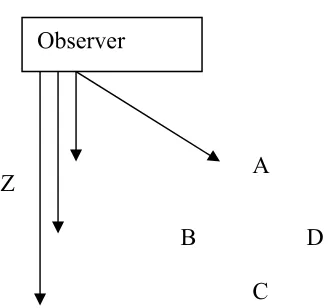
is the angle of deviation of the object from the horizontal ... 2Figure 2: B, C and D are below A from the observer's perspective. ... 5
Figure 3: A representation of behind with A being the observer and behind being behind the circle. ... 5
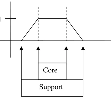
Figure 4: Core and support of a fuzzy set ... 12
Figure 5: convex fuzzy set (left) and non convex ... 13
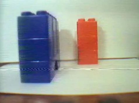
Figure 6: block configuration for the robot's camera (red block is on the right). ... 16
Figure 7: Block configuration with the blue blocks at a slant. ... 16
Figure 8: Triangle formed from distance readings and compass readings from the robot in a bird’s eye view. ... 18
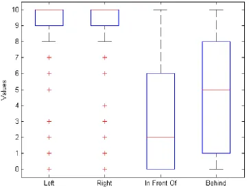
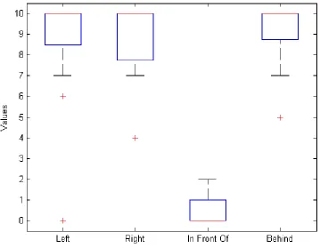
Figure 9: Box plot of survey results. ... 21
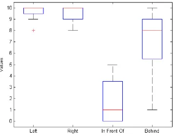
Figure 10: Box plot of survey questions where the block was more "behind" ... 22
Figure 11: Box plot of survey question where blocks were close to "right" and "left". .. 23
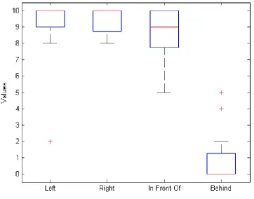
Figure 12: Box plot of survey question answers where the block is more "in front of". . 24
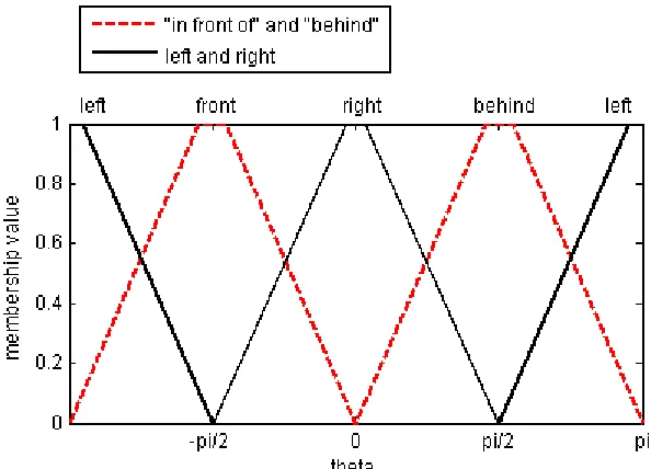
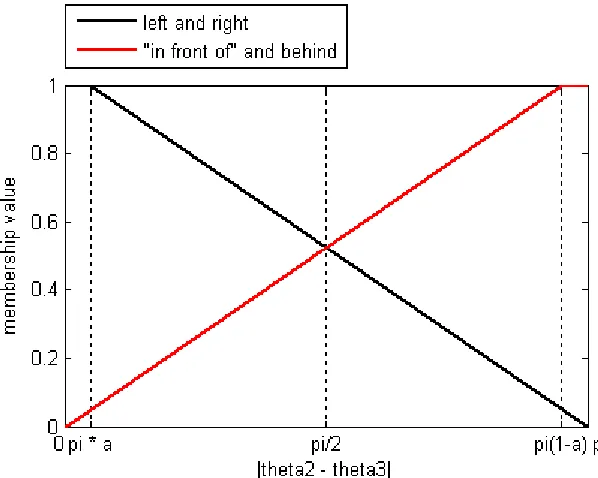
Figure 13: Plot of membership functions as they relate to the angles, traditional method. . ………26
Figure 14: Plot of membership functions reflecting the angles within a triangle ... 27
Figure 15: Angle Aggregation comparison for the relationship “In Front Of” ... 30
Figure 16: Centroid comparison for the relationship “In Front Of” ... 31
Figure 17 - Histogram of Angles comparison for the relationship “In Front Of” ... 31
Figure 18: Example of not "In Front Of". Also an example of “Behind” ... 32
Figure 19: Example of "In Front Of". Also an example of not “Behind” ... 32
Figure 20: Angle Aggregation comparison for the relationship “Behind” ... 34
Figure 21: Centroid comparison for the relationship “Behind” ... 35
Figure 22 - Histogram of Angles comparison for the relationship “Behind” ... 35
Figure 23: Angle Aggregation comparison for the relationship “Right”. ... 36
Figure 24: Centroid comparison for the relationship “Right” ... 37
Figure 25 - Histogram of Angles comparison for the relationship “Right” ... 37
Figure 26: Example of less to the "right". Also an example of less to the "left" ... 39
Figure 27: Example of more to the "right". Also an example of more to the "left". ... 39
1. Introduction
As we attempt to create a new generation of automated helpers to solve problems in the military, in elder assistance, transportation, and other areas, we increasingly find that we need robots that can interact naturally with humans. Ultimately this interaction will have to include more natural language (spoken language) to simplify the communication between human and robot. Consider the scenarios below.
Scenario One: An autonomous robot is searching for survivors after a recent high magnitude earthquake. The robot snakes along in crevices too small or too dangerous for a person. Due to the debris, communication is intermittent with a human operator. At one point deep into the search, all communication is lost, but the robot continues its mission. The robot
periodically calls for survivors that may be hidden from view. The robot detects a shout of a survivor after one of its own calls. The survivor cries out “I’m over here, behind the red drink machine, kind of to the left of the blue support column.” The robot calculates the likely position of the survivor, finds the person, drops off a survival package and heads back to within transmission range to report the location.
forward of it.” After a few minutes the scout robots detect the sniper and the soldier calls in a small missile strike.
As the scenarios above illustrate, spatial relationships are crucial to human robot interaction. Without their use it is almost impossible for a person to direct a robot to move through its environment using spoken language. In the first scenario, the robot would not be able to locate the survivor, and in the second the soldier would not be able to control multiple robots. The challenge here is enabling the robot to understand spatial relationships as a person would.
The scenarios above describe the use of spatial relationships in the real world. Spatial relationships describe the relation of one object to another. Since spatial relationships
typically involve direction and magnitude they naturally lend themselves to the use of vectors [8], where the angle of deviation plays an important role. Typically the angle of deviation is taken from the horizontal reference as in Figure 1, below.
Figure 1 -
α
is the angle of deviation of the object from the horizontalThis thesis identifies and evaluates techniques for determining the spatial relationships between two objects from an observer’s perspective. This will involve triangle geometry and not just one angle from a reference line, as has commonly been assumed in past modeling research.
It is a straightforward task for a human controller to control a robot with a joystick (where a joystick is simply a representative continuous pointing device), in which case the robot has
little autonomy and is simply an extension of the controller. In the first scenario above it is virtually impossible for a human controller to be directly involved because the robot must act autonomously in some situations. In the second scenario, difficulties are exacerbated by the presence of multiple robots that move simultaneously. These robots need to be able to
interpret and act upon spoken commands. In order for this to happen it is crucial for the robot to understand the language of spatial relationships. This presents a challenge since spatial relationships are inherently imprecise. The phrase “the desk to the left of you” can
encompass a rather large area. There are also terms such as “directly to the left” or “to the left and a little in front of” which introduces more uncertainty. Such imprecision often does not lend itself well to rigorous mathematical analysis. The mathematics of fuzzy set theory addresses such imprecision by its use of membership functions. In this paper we will develop and compare three fuzzy logic methods for determining spatial relationships.
A considerable amount of research has been conducted on spatial relationships [1 – 2, 6, 9 – 12, 14]. Much of this research is accomplished by using a bird’s eye view of the scene, which gives complete knowledge of the size and shape of the objects under consideration in a 2d world. The amount of research exploring a person’s or robot’s point of view is not as rich [3, 4, 16]. In these limited viewpoint situations, only knowledge of the size and shape of the part of the object facing the observer is available, which may be only the tip of the iceberg. An observer’s initial assumption about the spatial relationship between two objects may be completely wrong and yet recognizable as being wrong only once the entire object is
observed. And yet that initial assumption is all that is available to begin with. In this research we will compare three different methods of calculating spatial relationships in these
In section 2 we detail spatial relationships, giving a history of previous research and what aspects are important to this research. Section 3 gives a basic survey on other previous research related to robotics and fuzzy logic which gives a general feel for the current state of the science. This section also shows that there is a need for more research in uncertain spatial relationships from an observer’s perspective. Following is a general introduction to fuzzy logic and how it relates to spatial relationships. The three fuzzy logic methods are detailed and how they are modified for the spatial relationships between two objects from an observer’s perspective. From there the general format of the experiments is explained and how the human survey was conducted. Finally the results are presented and analyzed. The thesis ends with a discussion of limitations and possible areas for future research.
2. Background
2.1 Spatial Relationships
In this section we will concentrate on the research that deals with linguistic interpretations and robotics. The semantics of spatial relationships is considered to be of the closed class form, meaning the spatial relationships is one of the foundational organizing structures on which further conceptual material, such as complex language, is built [13]. Closed class forms contain relatively few items and add new members rarely. As a closed class form, spatial relationships have commanded considerable fascination.
Some of the basic research deals with using vector algebra to determine spatial relationships
in language [12]. For instance given two objects A and B and vector AB →
Figure 2: B, C and D are below A from the observer's perspective.
Behind is defined as applying to objects for which the magnitude of a vector from A to the
object is greater than the vector AC →
in Figure 3, and the angle of the vector is less than the
angle of the vector AD →
.
However, this is a restrictive definition, because any object a little bit outside of the angle of
the vector AD →
can still be considered “mostly behind” the circle. The survey data in this research show the limitation of this discrete approach, in practice. Fuzzy logic helps to remedy the restrictiveness.
The acceptability of spatial terms to object diagrams has been explored before. Regier and Carlson [14] give a summary of this research. Earlier research in this area uses spatial templates to categorize linguistic terms based on vector data. Regier and Carlson introduce
Observer
Z A
B
C D
A B
C D
the terms landmark for the object where the spatial relationships are being determined from, and the trajector as the object being used for the spatial relationships to. One of the earliest techniques used for determining spatial relationships is the bounding box method [14]. The bounding box defines an area directly above the landmark which is bounded by area of the landmark for the relationship “above”. This is accomplished by determining the vertical and horizontal centeredness of the trajector with respect to the landmark by using sigmoidal squashing functions. The sigmoidal functions return a value between 0 and 1, 0.5 being ideal for the spatial relationship, with some flatness in the curve around 0.5. The center of mass model calculates the center of mass of the landmark and the trajector and uses the angular deviation from the two objects to determine the relationship. The sigmoidal squashing
function is again used to give the values more of a curve to avoid abrupt transitions from 0 to 1. The proximal method is similar in using angular deviation but uses the point of the
landmark and the trajectory that are closest to each other. The hybrid model uses both the proximal and center of mass methods but also takes into account the height of the two objects. Instead of using a sigmoidal squashing function, a linear function is used that takes into account slope and the y-intercept for the alignment where the slope and y-intercept can take on any value that describes the line describing the relationship, or orientational
alignment. The Attentional Vector Sum (AVS) technique uses research into human
perception to add to the hybrid technique. The AVS method weights the vectors going from the landmark from the trajector by an attentional value. This attentional value is high when the vector is closely aligned to vertical between the landmark and trajectory for the
relationship “above” and low when the vector is less vertically aligned. The weighted vectors are then summed. To represent an attentional drop off they use a function to decay the values which is influenced by the distance between the the two objects.
Regier and Carlson compare the AVS technique with the Bounding Box, Proximity/Center of Mass model and the hybrid model. The AVS model performed the best since it uses
point of view, however, since they assume complete knowledge of the size and shape of the objects.
Using fuzzy logic is a more recent development in computing spatial relationships, starting in the mid 1990’s. I. Bloch gives a good summary of fuzzy logic and spatial relationships in general [2]. Keller and Wang compare three of the methods with simply intuitive
understanding of spatial relationships [10]. The three methods compared in this paper are those used by Keller and Wang, with a change of the compatibility method to a composition method. Most recently, Matsakis and Wendling introduce the concept of force histograms, which parse the objects into longitudinal sections with the thought that the sections of one object forces the object towards the sections of another object [11]. A longitudinal section is considered as being all the points along a vector that intersects an object. The more points in a section that intersect both objects the higher the weight of that section in a weighted mean. In this respect the histogram of forces is similar to the angle aggregation method. The results of the histogram of forces is only evaluated against intuition but seems to give satisfying results.
Gapp [6] uses human survey data to determine the importance of distance and angular data in the perception of spatial relationships. The experiments were designed to allow for the independent evaluation of distance versus angle to determine how much bearing each had in the perception of spatial relationships. Gapp discovered that angular deviation is the critical point in establishing spatial relationships. The scale of the angle is influenced by the
extension of the landmark object from the original size; so the larger the object the larger the area for each spatial relationships relative to the landmark. Also, the “in front of” and
“behind” relationships were rated higher than the “left” and “right” relationships, meaning the participants tended to give more credence to “behind” rather than “right”.
between the robot and other objects for navigation using linguistic descriptions. The simulated robot uses a ring of 16 sonar sensors to detect objects in the environment. The robot does not differentiate between objects and objects that are too close together for the robot to navigate between are considered one object. The vertices of the detected objects are used as the boundaries for input into the algorithm as vectors. Several experiments are performed where the robot is able to generate linguistic expressions such as “The object is forward and slightly to the right of the robot” in a satisfactory manner. The research does not extend to spatial relationships between objects or comparing the force histogram results to human perceptions and are only performed in simulation.
2.2 Other Related Spatial Relationship Research
Keller and Wang [9] attempt to learn spatial relationships using human intuition as a starting point for the training values into a neural network. The methods used as input into the neural networks are the centroid, angle aggregation and compatibility methods. The purpose of this is to learn the best values for the spatial relationships in order to generalize them for practical use. The neural networks performed well, but the researchers conclude that more work is needed with better input for training to find values in line with human perception. Complete knowledge of the objects is given to the algorithms.
Discovering uncertainties in geometric features in objects for possible use in robotics was the focus of work by Durant-Whyte [4]. Each geometric feature is considered a set of stochastic points which is represented by a Gaussian distribution. The distributions represent
uncertainty functions which then can be manipulated or combined. In the research probability distributions are used to find the likely geometric feature of an object based on known
features for use in combining data from different coordinate systems or different sets of sensors or viewing an object from another location.
representation of fuzzy sets is created. Then the fuzzy landscape around the landmark is compared with the trajector. This method works well for structural pattern recognition with imprecise information, such as in identifying patterns in an image such as an MRI or facial recognition. The reasoning behind the approach is that when extracting structures from an image, the structures are inherently imprecise, meaning they do not have well defined boundaries. This situation thus lends itself to fuzzy sets. This method can also be used for 3D images. This research does not extend, however, to cases in which only part of an object can be perceived from an observer’s perspective.
Simultaneous Localization and Mapping (SLAM) is used in the work of Huang et al. [7], where only a camera is used to sense relative positions of object. The motivation here is that most cameras are inherently noisy so object location can be represented by a probability density function. The assumption is that the object position is uniform when distance information is not available. At first the probability density function is uniform, and then is updated as additional information about the environment is discovered, though the spatial relationship between objects is not calculated in this paper.
Dehak et al. [3] propose a system for spatial reasoning with uncertain information where spatial reasoning in this case is relating the relationship of two points given how they relate to a third point. Probability methods are used where only angular data is known. The authors suggest that the application for this research would be for localization, such as a cell phone finding its position in a city where there are two known landmarks nearby.
2.3 Fuzzy Set Theory As Zadeh observed:
“Clearly, the "class of all real numbers which are much greater than 1," or "the class of beautiful women," or "the class of tall men," do not constitute classes or sets
Classical propositional logic deals with true and false, something is true unless it is not true which is false. This also is the law of the excluded middle. Instead fuzzy logic deals with membership grades in fuzzy sets. For instance a man who is 6’1” might be considered tall with a fuzzy value of 0.7. The set is tall men. The fuzzy value is not to be confused with probabilities, the value 0.7 does not mean the man has a 0.7 probability of being tall but that the man has a 0.7 membership grade in the set of tall men. So fuzzy values take on the range of values of [0,1]. A value of 1 means the object absolutely belongs to the set, 0 is absolutely not and everything else in between has varying degrees of membership. To relate fuzzy logic to spatial relationships, a proposition such as “the ball is to the left and slightly in front of you” might actually take on the values of 0.8 for “to the left” and 0.2 for “slightly in front of you”. Traditional sets are also called crisp sets in that values either belong to the crisp set or they don’t. So a fuzzy set memberships function that always returns 0 or 1 for it’s
membership value is a crisp set, or a crisp set can be considered a special case of a fuzzy set [14]. Fuzzy set theory is an extension of crisp set theory and as such expresses the laws of normal set theory since set theory is the basis of most mathematics such as the Indempotent law, Commutative law, Associative law, Distributive law and De Morgan’s law.
Fuzzy set values are calculated using a membership function. These membership functions can take on any shape such as a straight line, triangle, trapezoid or Gaussian distribution. One example of a triangle shaped fuzzy set function is below:
2 , 2 0
2 ( )
2 ,0 2
x x x A x x x
µ
+ − < <
= −
≤ <
(1.1)
µ denotes the fuzzy set membership function where µA( )x is the membership function
The union or intersection of fuzzy sets can be calculated a number of ways, the most typical would being via the max or min operators. The most important consideration when deciding on a union or intersection operation is to take into account the laws of Commutativity, Monotonicity, and Associativity. If the max operator is used for the union operation and the min for the intersection, then an example would be:
( ) {0.1,0.4,0.4,0.3,0.2,1,0.9} ( ) {0.2,0.5,0.3,0.8,0.1,0.4,1}
( ) ( ) ( ) max( ( ), ( )) {0.2,0.5,0.4,0.8,0.2,1,1} A
B
A B A B A B
x
x
x x x x x
µ
µ
µ
∪µ
µ
µ
µ
= = = ∨ = =And intersection would be:
( ) ( ) ( ) min( ( ), ( )) {0.1,0.4,0.3,0.3,0.1,0.4,0.9}
A B x A x B x A x B x
µ ∩ = µ ∧ µ = µ µ =
As noted above the union and intersection operations are equated with disjunction and conjunction respectively. The complement of A, above, is:
( ) 1 A( ) {0.9,0.6,0.6,0.7,0.8,0,0.1}
A x x
µ
= −µ
=Figure 4: Core and support of a fuzzy set
As can be seen from the figure, the support is the full range of the fuzzy set where the value is greater than 0 [5].
The α-cut for a fuzzy set is defined as a division of the fuzzy set. α is established as a value between (0,1] and all fuzzy set values greater than or equal to α are set to 1 and all other membership values for the fuzzy set are set to 0. For instance if we have the crisp set of values:
A = {1.0, 0.9, 0.9, 0.7, 0.5, 0.2, 0.1}
then an α-cut is:
Aα = A0.9 = {1, 1, 1, 0, 0, 0, 0, 0}
Alpha cuts are generally used to decompose fuzzy sets into rectangular regions and can be used to transform a fuzzy set into a crisp set.
A fuzzy set is normal if its maximum fuzzy value is 1. A fuzzy set is convex if the fuzzy set is monotonically increasing or monotonically decreasing or monotonically increasing then monotonically decreasing (Figure 5), or on the relation x < y < z then:
( )y min[ ( ),x ( )]z
A A A
µ
≥µ
µ
. [14]Core
Figure 5: convex fuzzy set (left) and non convex
t-norms are a generalized form of the 2-valued conjunction for fuzzy logic and can be used for intersection operations as in crisp sets. So the t-norm function is T:[0,1] x [0,1] →[0,1] and satisfies the properties of Commutativity, Monotonicity, Associativity. The t-conorm is a generalized form of the logical disjunction for fuzzy logic and can be used for union operations. The t-conorm satisfies the properties of Commutativity, Monotonicity, Associativity and identity element. [2]
Fuzzy sets use symbols to represent an entire set. For the discrete set an example of a single value of a fuzzy set is: 0.3/5 which simply states for the value 5 the fuzzy value is 0.3. The generalized version is: µA( )/x x which states for the value x the fuzzy value is µA( )x on the set
A. For a discrete set the general case is represented as follows:
( )1 ( )2 ( )
...
1 2
1
( )
n x x
xn
A A A
A i x x xn
i
x
µ
µ
µ
µ
= + + +=
∑
(1.2)And for the continuous case:
( )/
A
A
x
i
x
i
x
µ
=
∫
(1.3)
In a real world example the discrete case would look like:
0.4 0.3 0.1 0.3 1
1 4 2 4 6
The “/” and “+” above are not literally division and addition symbols but are used as separators [5].
Linguistic hedges are terms such as “very”, “slightly”, or “a lot” that modify or intensify another term such as “old”, “young”, “tall”, etc. In fuzzy logic these are described as “concentrations”. To calculate such terms in fuzzy logic a modifier is added to the calculation, for instance, if the original fuzzy set is represented by A, then adding the modifier “very” to A might be used as follows:
(
)
22
"Very"A A ( ) /x x i
x
µ
= =
∫
(1.4)There are some standard forms of linguistic hedges such as “very” shown above, but the exact calculation modifier chosen may depend on the application and can be somewhat subjective. There are certain categories for the calculation of linguistic hedges. Dilations stretch, or increase the membership value in the fuzzy set. Erosion decreases the membership in the fuzzy set. [17]
The extension principle maps one fuzzy set to another by way of a mapping function. If we have fuzzy sets A and B with function f:X→Y where X is in A and Y is in B, then to relate the fuzzy sets:
-1 sup ( ) ( ) f ( ) ( )
( ) -1
0 f ( )
x y
A y f x y f A y
µ
µ
≠ ∅ = = = ∅ (1.5)Where f−1( )y is the inverse image of B by f. For instance if you have the following fuzzy set and function:
4
1
0.1 0.4 0.8 0.2 ( )
2 3 4 5
( ) 2 2
A i
x
f x x
µ
=
= + + +
= +
Then f(x) can be considered a mapping function into Y which creates:
4
1
0.1 0.4 0.8 0.2
( )
6 8 10 12
A i x
µ
= = + + +∑
The above fuzzy set could also be read as “about 10” and the previous one as “about 4”.
An application of the extension principle is the compatibility of fuzzy sets as used in the histogram of angles – compatibility method [5].
The composition of fuzzy relations is defined as:
( )y max[ ( )x ( , )]x y
A R x X A R
µ
o = ∈µ
∧µ
(1.6)Where A is a fuzzy set on X and R is a fuzzy relation on X ×Y. The composition of A and R, denoted A oR, is a fuzzy set on Y. If the fuzzy relation is represented as a matrix and the fuzzy set as a vector then the composition can be illustrated as follows:
1 2 1
1 2 3
( ) ( ) ( ) ( ) ( ) ( )
2 3
y y x d e x x x
a b c x f g a d b f c h a e b g c i h i x = ∧ ∨ ∧ ∨ ∧ ∧ ∨ ∧ ∨ ∧ o
Where the ∧ is often calculated using the min operation and the ∨ is often calculated using the max operation. [14]
3. Generating the robot sensor data
For this experiment there were two blocks. One was a long, rectangular, blue block; the other was a shorter, square, red block. The blue block was three time longer than the red block and both were the same width. The two blocks were placed in a total of 30 different
straight line towards the robot. The advancements were performed six times until the red block was approximately one red block length in front of the blue block. After the six advancements the blue block was rotated by approximately 18 degrees and the advancement of the red block was repeated as before. This continued until the blue block was at a 90 degree angle from its former position.
Below are two pictures taken from the robot that illustrate the blocks and the configurations.
Figure 6: block configuration for the robot's camera (red block is on the right).
Figure 7: Triangle formed from distance readings and compass readings from the robot in a bird’s eye view.
1.record compass reading
2.Take a snapshot for survey picture 3.Identify red object
4.Calculate rotation needed to center on left edge of red object
5.Rotate to left edge 6.If within threshold
a.record compass reading b.record distance reading
7.else
a.repeat 4-7
8.Repeat 4-8 for center and right points 9.Repeat 3 – 8 for blue object
One additional control was added to reduce the noise in the sensor data. The compass sensor was averaged over ten readings, as it tended to vary by small amounts between individual readings. The infrared distance sensor was tested for volatility of the readings. Five distance readings were compared and if any two or more differed from the others by more than 20mm then the readings were discarded and new ones were acquired. The distance readings were also averaged once an acceptable set of five were obtained, discarding the outlier if it existed.
As shown in Figure 8, below the readings form part of a triangle. The robot is represented by the green colored rectangle at the bottom. The initial two distance readings are r1 and r2 and
Figure 8: Triangle formed from distance readings and compass readings from the robot in a bird’s eye view.
Object A contains the points { , , }al ac ar and like wise object B contains the points
{ ,bl bc,br} where l, c, and r represent left, center and right respectively. There are a total of
9 pairs of angles to consider between all the points on objects A and B.
1
θ
andθ
2 are calculated from triangle formula to find an angle as follows:2 2 2
2 3 1
, arccos
1 2 2 2 3
r r r
r r
θ θ
+ −
= (1.7)
2
r is calculated from the triangle formula to find the third side of a triangle as follows:
2 2 2 cos( )
3 1 2 1 2 3
r = r +r − r r θ
(1.8)
4. Generating the Survey Data for Validation
The purpose of human subject testing is to compare the three fuzzy logic methods interpretation of the spatial relationships with human perception in order to validate the methods. This was accomplished by using the pictures of objects taken by the robot and presented to survey participants. For this survey 30 pictures were chosen with various configurations of the 2 objects. The first page of the survey reads as follows:
Spatial Relationships Survey
• This is a short survey for research into spatial relationships and robotics
• You will be shown a series of 31 images each with 4 questions asking you to rate
how well the question describes a picture on a scale of 0-10. 0 being the worst and 10 being the best.
• Treat each image independently, in other words don't wait for a best or worst, it may not exist. Just pick the most appropriate rating for the question based on the current image.
• 0 means the sentence does not apply.
• Simply use your best judgment.
• DO NOT go back to change an answer.
• Take the survey only once!
• Once you start, please try to complete the survey in its entirety
• The survey should take at most 20 minutes to complete.
Thank You for you participation.
How well does each of the questions below describe the picture above, 0 being the worst and 10 being the best:
The red blocks are to the right of the blue blocks:
0 1 2 3 4 5 6 7 8 9 10
The red blocks are in front of the blue blocks:
0 1 2 3 4 5 6 7 8 9 10
The red blocks are in back of the blue blocks:
0 1 2 3 4 5 6 7 8 9 10
The blue blocks are to the left of the red blocks:
0 1 2 3 4 5 6 7 8 9 10
Figure 9: Box plot of survey results.
Figure 10: Box plot of survey questions where the block was more "behind"
Figure 11: Box plot of survey question where blocks were close to "right" and "left".
Figure 12: Box plot of survey question answers where the block is more "in front of".
Figure 12 shows a box plot of a survey question’s answers where the block is more “in front of” the other. Once again the answers are pretty consistent. There is one extreme outlier on “left” that may be due to not understanding the question. Here human judgment is not quite as certain of “in front of” as in “behind” in figure 10. There is no explanation for this, but the difference is small enough that it is still reasonable and intuitive.
5. Predicting the Spatial Relationships
5.1 Angle Aggregation Method of Fuzzy Values
The Angle Aggregation method is outlined in [10] but will be repeated here for
apex, or maximum value, of the spatial relationship is considered to be around 0 for the relation “right” with the other relations moving counterclockwise around the axis. Based on this definition most spatial relationships can be defined in terms of angular measurements. If we define two points A and B where A is on object one and B is on object two then θ would normally be the angle between the line AB and the horizontal axis. However, since we are determining angles in the triangle from the robot’s perspective the fuzzy membership function changes from:
1 / 2
/ 2
( ) / 2 / 2
/ 2(1 )
0 / 2
a a RIGHT a a
θ
π
π
θ
µ
θ
π
π
θ
π
θ
π
< − = − ≤ ≤ > (1.9) To: 1 2 1 21 2 1 2
1 2 1 ( ) (1 ) 0 , a a RIGHT a
θ
θ
π
π
θ
θ
µ
θ θ
π
π
θ
θ
π
θ
θ
π π
− < − −= − ≤ − <
− = −
(1.10)
they become less to the right or to the left of each other and more “in front of” or behind. The relationship for left is the same since they are symmetric within the confines of the triangle, in other words if one object one is to the left of object two then object two is to the right of object one by the same degree or BRIGHTA = ALEFTB.
The function for “in front of” and “behind” is:
1 (1 ) 1 2
1 2
( , ) 0 (1 )
_ _ 1 2 (1 ) 1 2
0 1 2 0
a
a n
IN FRONT OF a
π θ θ θ θ µ θ θ π θ θ π θ θ
− < − −
= − < − ≤ −
− =
(1.11)
The membership functions can be graphed as Figure 13 shows in the traditional sense with negative values for angles.
Figure 13: Plot of membership functions as they relate to the angles, traditional method.
Figure 14: Plot of membership functions reflecting the angles within a triangle
To compute the aggregated angles consider A and B as two image regions (i.e. the two object in the robots vision) the fuzzy value for each pair of members θ(a,b) is computed,
( ( , ))
_ _ a b
A REL B
µ θ . Then an aggregation operator is used to calculate the fuzzy
relationship for each pair. There are many such aggregation operators. The one used here is the generalized mean operator defined as:
1
( ,...,1 ; , 1,..., ) 1
1 1
p
n p n
g n p w wn wi i where wi
i i
µ
µ
µ
= ∑ ∑ =
= = (1.12)
5.2 Centroid Method
The method used here to calculate the centroid method is the simplest where a characteristic point is chosen from each object, in this case the center to center, and the angles in the triangle used to calculate the relationship. [2] Let cA and cB represent the object centroids of objects A and B. Then the fuzzy membership function in the normal usage for the relation is defined as:
( ) ( ( , ))
B A c c
A B
RIGHT right
µ = µ θ (1.13)
In the triangle where the spatial relationship is between two observed objects the formula becomes:
( ) ( , )1 2
B A
RIGHT right
µ = µ θ θ (1.14)
Where the difference between the two angles is computed in the membership function. Once again it is important to distinguish which object is the landmark and which is the trajector for the left and right relationships.
5.3
Histogram of Angles – Composition Method
The composition method is closely related to the compatibility method except that
composition of the fuzzy distribution with the fuzzy relation is used instead of compatibility as explained below. For this method the membership functions are given by trigonometric
functions calculated from the angle difference between θ2 and θ1. The original research [10] uses the formula for the relationship RIGHT:
2
cos / 2 0 / 2
( ) 0 RIGHT otherwise θ π π µ θ − ≤ ≤ = (1.15)
2 1 2
cos / 2 0 / 2
2 ( , )1 2
0 RIGHT otherwise θ θ π π µ θ θ − − ≤ ≤ = (1.16)
The difference of the angles must be divided by 2 as it can approach
π
. The same formula is used for LEFT but with the angles reversed. The membership function for IN FRONT OF is:_ _
2 1 2
sin / 2 0 / 2
2 ( , )1 2
0
IN FRONT OF
otherwise θ θ π π µ θ θ − − ≤ ≤ = (1.17)
BEHIND is defined similarly.
Let Θ represents the collection of the difference of all angles θ θ(1 − θ2) where
1
θ represents the angle on object A and θ2represents the angle on object B. There may be
angle values within Θ that are the same. The angle values were rounded to two digits to create multiple angles of the same value. The frequency of each angle is counted resulting in a histogram of angles H(A,B) = {(θ,f)}, where f is the frequency of the angle. The frequency
of the angles in the histogram is then divided by the maximum frequency to normalize the values.
6. Results
6.1 Robustness to Sensor Noise
One of the issues that can arise in the application of a theoretical transformation technique to physical data is sensitivity to noise. If sensor readings are all within a narrow band, then a given transformation technique may produce reliable results, but outside that band it may not. Our first test of the fuzzy techniques is of this possibility.
For comparison purposes a theoretical model of the angle values was created. The theoretical model represents the measurements if the robot was able to obtain ideal measurements. The theoretical model is then compared with the robot sensor data. If the difference between the two models is great, then it may have indicated a flaw in the way the robot gathered sensor readings.
Below are graphs for the three fuzzy logic methods comparing theoretical model, sensor model and survey data for the spatial relationship “In Front Of”.
Figure 16: Centroid comparison for the relationship “In Front Of”
The trial numbers on the x axis represents each of the configurations of blocks. Each trial number corresponds to a particular configuration of the blocks.
Figure 18: Example of not "In Front Of". Also an example of “Behind”
Figure 19: Example of "In Front Of". Also an example of not “Behind”
As can be seen in the graphs, there is not a marked difference between the robot sensor data and the theoretical model. The difference between the models that does exist can be
attributed to the uncertain readings of the robot sensor data.
visible to the robot in this set of trials, only a slim section of the side is visible. However this side of the blocks is apparent in the pictures as can be seen in Figure 18, above. This effect of not seeing the side of the blocks minimizes the angles that point towards the relationship of “in front of”, mostly in the early trials when the long side of the blocks has the smallest profile to the robot.
The next apparent feature is the histogram of angles method comes closer to matching the human survey data than the centroid or angle aggregation methods. The histogram of angles tends to give a more optimistic view of the data. If we take a particular instance of a trial such as trial 18 (the highest spike) and look at the actual data we can see the logic behind this. The trial 18 data is as follows:
Normalized histogram: H = [1 1 1 1 1 1 1 1]
Fuzzy Relationship:
R = [0.296208 0.53973 0.82248 0.257214 0.481956 0.769586 0.182512 0.382734 0.681592]
Then taking the composition H o R:
[(1 0.296208) (1 0.53973) (1 0.82248) (1 0.257214) (1 0.481956) (1 0.769586) (1 0.182512) (1 0.382734) (1 0.681592)] 0.82248
∧ ∨ ∧ ∨ ∧ ∨ ∧ ∨
∧ ∨ ∧ ∨ ∧ ∨ ∧ ∨
∧ =
This is an extreme case as each angle value only occurred once but it displays the general optimism of the histogram of angles – composition method. With only nine angles in the set the highest occurrence of an angle in any one set was three. In a few of the trials each angle only occurred once. The composition method favors the fuzzy values for angles that occur more frequently.
method chooses the center point on object A to the center point on object B as the characteristic point which ends up closely resembling the angle aggregation method.
Figure 21: Centroid comparison for the relationship “Behind”
Above are the comparisons of the various fuzzy logic techniques of the theoretical and robot models for the spatial relationship “behind”. Once again the composition (histogram of angles) method seems to most closely resemble the survey data. This is due to the composition method favoring the angles that occur most frequently as explained above.
In this instance the theoretical model actually performs worse than the actual robot sensor data. Again this is due to the robot not sensing the side of object A (the blue blocks on the left) which give a larger contrast between the angles from A to B. The right point of the theoretical model is on the right side of object A that the robot can not detect thus giving less of a contrast between the angles.
Figure 24: Centroid comparison for the relationship “Right”
Above are the comparisons of the various fuzzy logic techniques of the theoretical and robot models for the spatial relationship “right”. In the robot sensor model the peaks and valleys in the graph for the fuzzy logic techniques are much more pronounced than in the previous spatial relationships. Once again this is mostly due to the pronounced difference in angles of the robot’s inability to detect the side of the blue, A block on the left. The theoretical model does a better job of predicting the survey data since the right side point is on the side the robot cannot detect. This is apparent in Figure 18, above.
The histogram of angles method gives a slightly lower estimation on the robot sensor data in
trial one in Figure 25, above. This is caused by the use of the cos2
θ
formula. Around trials 7 and 8 the histogram method peaks much higher than the centroid or angle aggregation techniques. The angle data for the difference between the right point on object A and the points on object B is much smaller than the other points, giving a larger value for the2
cos
θ
formula. The centroid method does not use these points for its characteristic points and the mean of the angle aggregation technique mitigates the contrast in the values.Figure 26: Example of less to the "right". Also an example of less to the "left"
6.2 Sum of Squared Errors Analysis
Table 1: Sum of Squared Errors computed against the survey data.
Sensor Data Theoretical “In Front Of”
1. Angle Aggregation 2. Centroid
3. Histogram of Angles
1.826 2.119 1.122 2.332 2.889 1.267 “Behind”
1. Angle Aggregation 2. Centroid
3. Histogram of Angles
0.929 0.748 0.783 2.801 2.246 2.224 “Right”
1. Angle Aggregation 2. Centroid
3. Histogram of Angles
3.911 4.207 2.883 1.239 1.485 0.259 “Left”
1. Angle Aggregation 2. Centroid
3. Histogram of Angles
3.851 4.125 2.951 1.188 1.427 0.266
For the sum of squared errors, the difference was computed between the models above with the survey data. The important fact to remember is that we are trying to come as close as possible to how a person might perceive the spatial relationships in the picture.
The first obvious feature of the table above is how much better the sensor data performs than the theoretical model on the spatial relationship “behind”. This is especially true on the first set of trials where the longer blue block on the left is facing straight towards the observer. Here the robot can not detect the longer side of the blue block (Figure 18), so all
measurements are from the front of the block. This gives a larger deviation in the angles from one block to the other, thus giving a better match on “behind”. In later trials this effect is less pronounced but is still apparent.
point, in this case the center point that was computed by the robot. This point typically gives a larger deviation for the angle then averaging or composing all the angles. This is the only place the centroid method performs well, all other places in either model the centroid method does not perform well.
None of the fuzzy logic methods performs very well with the left and right spatial
relationships. Here human perception comes into play. As long as one object is within the bounds of another object, a person gives significant credence to right and left relationships as show in figure 28.
Figure 28: As long as one object is in the bounds of another, a person will classify as "right" or "left" with a high degree of confidence.
The angle measurements, however, create a deviation that prevents the classification with such a high level of probability.
The final apparent attribute to the sum of square errors analysis is the performance of the histogram of angles. This is due to the optimistic behavior of the composition of the histogram with the fuzzy set relationship as explained the in previous section.
7. Conclusions
perceptions. This paper compared three fuzzy logic techniques with human survey data to find if any of the techniques performed acceptably against human perception. These techniques have been used for allocentric, or bird’s eye, views in previous research but not with egocentric views which creates uncertain data.
In general human perception places an object to the right or the left of another with a high degree of certainty when the object is to the right or left even when the object is slightly in front or behind as well. This creates a marked difference in the fuzzy logic techniques with the survey data as the curve used by fuzzy logic techniques on the angle values puts the objects to the left or right with a lower fuzzy value. This will have to be addressed in future research to modify or create a technique that gives a more optimistic value in such cases. Also using more accurate sensors or vision capabilities on the robot could help as well in detecting the full observable area of the object. Part of the effect could be due to the
observations in [6] where the “in front of” and “behind” relationships had more emphasis to an observer in a bird’s eye view. In this case it could be possible that the “left” and “right” had more emphasis in the first person view.
In general, the histogram of angles – composition method gave the most satisfying results with favoring angles that occur more frequently and in giving more optimistic results,
especially with the “In front of” and “behind” spatial relationships. However, with the “right” and “left” relationships the histogram of angles still gave results that were somewhat
inconsistent with human perception. More work needs to be performed to find how these techniques and others behave when presented with more complex configurations of objects in the field of view.
8. Future Work
has discovered techniques in some of the other areas. One of the areas is in machine vision. One challenge is when one object is in front of another how does the robot distinguish one object from the other, especially if they are of similar color. This sort of machine vision research must be combined with the spatial relationship research in order to give a more complete picture of the environment.
Only four of the primitive spatial relationships were used here, there are many more that need to be addressed as well before a useful vocabulary can be utilized. Some of these
relationships are near, far, surround, inside, outside and with three dimensional scenes above and below. This should be considered the minimum before a meaningful exchange can occur between human and robot. There has been previous research into these relationships as well, some of which is addressed in the papers cited herein.
One more aspect for future research is what is the minimum amount of information the robot must know of the environment before being able to make accurate predictions about the spatial relationships for any given algorithm. Here we used three points on each object, left, center and right. With more points some the algorithms here may have had better
performance. Discovering an algorithm that uses a minimum of information is essential to speed a robot’s understanding of its environment.
The work presented here compares relatively straightforward methods of determining spatial relationships given the current scene available. But if the robot moves a new scene is
presented and any information from previous scenes is not incorporated into the current calculations of spatial relationships. This could play a part in determining spatial
9. References
1. Bloch, I.. "Fuzzy Relative Position Between Objects in Image Processing: A Morphological Approach." Pattern Analysis and Machine Intelligence, IEEE Transactions On 21.7 (1999): 657-664.
2. Bloch, I.. "Fuzzy Spatial Relationships for Image Processing and Interpretation: A Review." Image and Vision Computing 27.9 (2005): 89-110.
3. Dehak, S. M. R., Bloch, I., and Maitre, H.. "Spatial Reasoning with Incomplete Information on Relative Positioning." Pattern Analysis and Machine Intelligence, IEEE Transactions On 27.9 (2005): 1473-1484.
4. Durrant-Whyte, H.F.. "Uncertain Geometry in Robotics." Robotics and Automation, IEEE Journal Of 4.1 (1988): 23-31.
5. Dubois, D., and H. Prade. Fuzzy Sets and Systems: Theory and Applications. New York, NY: Academic Press, Inc., 1980.
6. Gapp, K. “An Empirically Validated Model for Computing Spatial Relations.” In Proceedings of the 19th Annual German Conference on Artificial intelligence: Advances in Artificial intelligence (September 11 - 13, 1995). I. Wachsmuth, C. Rollinger, and W. Brauer, Eds. Lecture Notes In Computer Science, vol. 981. Springer-Verlag, London, (1995) 245-256
7. Huang, Henry, Marie Frederic, and Narongdech Keeratipranon. "An Improved Probability Density Function for Representing Landmark Positions in Bearing-Only SLAM
8. Jones, Huw. Computer Graphics Through Key Mathematics. London: Springer, 2001.
9. Keller, J.M., and X. Wang. "Learning Spatial Relationships in Computer Vision." Proceedings of the Fifth IEEE International Conference On 1 (1996): 118-124.
10. Keller, J. M. and Wang, X. 1995. “Comparison of Spatial Relation Definitions in Computer Vision.” In Proceedings of the 3rd international Symposium on
Uncertainty Modelling and Analysis (March 17 - 20, 1995). ISUMA. IEEE Computer Society, Washington, DC, 679.
11. Matsakis, P., and L. Wendling. "A New Way to Represent the Relative Position Between Areal Objects." Pattern Analysis and Machine Intelligence, IEEE Transactions On 21.7 (1999): 634-643.
12. O'Keefe, J.. "The Spatial Prepositions in English, Vector Grammar, and the Cognitive Map Theory." Language and Space. Ed. P. Bloom. Cambridge, MA: MIT Press, 1996. 167-181.
13. Regier, T.. The Human Semantic Potential: Spatial Language and Constrained Connectionism. Cambridge, MA: MIT Press, 1996.
14. Regier, T., and L.A. Carlson. "Grounding Spatial Language in Perception: An Empirical and Computational Investigation." Journal of Experimental Psychology: General (1997).
16. Skubic, M.; Chronis, G.; Matsakis, P.; Keller, J., "Generating linguistic spatial descriptions from sonar readings using the histogram of forces," Robotics and Automation, 2001. Proceedings 2001 ICRA. IEEE International Conference on , vol.1, pp. 485-490, (2001).
17. Tanaka, K. An Introduction to Fuzzy Logic for Practical Applications. Niimura, T. New York, NY: Springer-Verlag, 1996
A.1 LEGO™ NXT Mindstorms
The Mindstorms NXT is a programmable robotics it released by LEGO™ in late 2006. It comes with the NXT brick, which is the main processor, four sensors: an ultrasound distance sensor, a touch sensor, a light sensor and a sound sensor, and three motors. The technical specifications for the NXT brick are as follows [1]:
• 32-bit ARM7 microcontroller
• 256 Kbytes FLASH, 64 Kbytes RAM • 8-bit AVR microcontroller
• 4 Kbytes FLASH, 512 Byte RAM
• Bluetooth wireless communication (Bluetooth Class II V2.0 compliant) • USB full speed port (12 Mbit/s)
• 4 input ports, 6-wire cable digital platform (One port includes a IEC 61158 Type
4/EN 50 170 compliant expansion port for future use) • 3 output ports, 6-wire cable digital platform
• 100 x 64 pixel LCD graphical display
• Loudspeaker - 8 kHz sound quality. Sound channel with 8-bit resolution and 2-16
KHz sample rate.
• Power source: 6 AA batteries
The ultrasound distance sensor was used for verification of the distance data. The Ultrasonic Sensor measures distance in centimeters and in inches. It is able to measure distances from 0 to 255 centimeters with a precision of +/- 3 cm. The Ultrasonic Sensor uses the same
Two motors were used to control the movement of the NXT. Each motor has a built-in Rotation Sensor. This allows precise control of the robot’s movements. The Rotation Sensor measures motor rotations in degrees or full rotations [accuracy of +/- one degree]. One rotation is equal to 360 degrees, so if a motor is set to turn 180 degrees, its output shaft will make half a turn. The built-in Rotation Sensor in each motor also allows different speeds for the motors and acceleration and deceleration parameters. The motors can also be
synchronized. [1]
In addition, two sensors from mindsenosrs.com™ were used, a compass sensor and an infrared distance sensor. CMPS-Nx is a digital magnetic compass specifically designed for NXT. The compass can be used as a digital sensor on NXT to detect deviation from magnetic north pole (heading). The compass sensor can be used to track a certain heading or follow paths with reference to magnetic north. This compass uses orthogonal two-axis magnetic sensor from Honeywell (HMC1052). The technical specifications are as follows [2]:
• CMPS-Nx V2.0 works with NXT-G, NBC/NXC, LeJOS and RobotC • Multiple reading modes (Byte/Int/Float)
• Dual sampling frequency (European/North American) • Resolution of 0.1 degrees with NBC and RobotC • Resolution of 1.44 degrees with NXT-G
• Intuitive command interface
• Maximum power consumption: 11.5mA at 4.7V
The infrared distance sensor was used as the main distance sensor for the experiments as its readings were found to be more accurate than the ultrasound sensor. Its technical
specifications are as follows [3]:
• Uses I2C bus digital interface to connect to NXT • Maximum current consumption: 30mA at 4.7V
For vision a NTSC wireless camera was mounted on the NXT and a USB digitizer was used to translate the picture to the PC.
Bluetooth communication was used to control the NXT from a PC, the PC being the master with the NXT as the slave. Bluetooth communication with the NXT is accomplished through the use of direct commands which are hex codes sent to the NXT using the I2C
communication protocol. The figure below shows the general telegram architecture [4]:
Byte 0 Byte 1 Byte 2 Byte 3 Byte N
Byte 0 – Command Type. The 7th lowest bit of this byte is used for identifying the command type. Currently the system has the following command types that need to be identified. Bit 7 (MSB) is used for indentifying whether the command should give a reply message or not.
• 0x00: Direct Command, reply required • 0x01: System Command, reply required • 0x02: Reply Command
• 0x80: Direct Command, reply not required • 0x81: System Command, reply not required
Byte 1 – Command byte. Used by the loader module to identify what should happen with the data. Open, Read, Write, Delete data, Direct communication with NXT.
Byte 2 – N – These bytes offer additional information.
Below is an example of the SETOUTPUTSTATE direct command which is used for controlling the motors [5]:
Byte 1: 0x04
Byte 2: Output port (Range: 0 – 2: 0xFF is special value meaning ‘all’ for simple control purposes)
Byte 3: Power set point (Range: -100 – 100) Byte 4: Mode byte (Bit-field)
Byte 5: Regulation mode (UBYTE; enumerated) Byte 6: Turn Ratio (SBYTE; -100 – 100)
Byte 7: RunState (UBYTE; enumerated)
Byte 8 – 12: TachoLimit (ULONG; 0: runforever)
Return Package Byte 0: 0x02 Byte1: 0x04 Byte 2: Status Byte
Valid enumeration for “Mode”;
MOTORON 0x01 Turn on the specified motor
BRAKE 0x02 Use run/brake instead of run/float in PWM REGULATED 0x04 Turns on the regulation
Valid enumeration for “Regulation Mode”;
REGULATION_MODE_IDLE 0x00 No regulation will be enabled REGULATION_MODE_MOTOR_SPEED 0x01 Power control will be enabled on
specified output
REGULATION_MODE_MOTOR_SYNC 0x02 Synchronization will be enabled (Needs enabled on two outputs)
Valid enumeration for “RunState”;
MOTOR_RUN_STATE_RAMPUP 0x10 Output will ramp-up MOTOR_RUN_STATE_RUNNING 0x20 Output will be running MOTOR_RUN_STATE_RAMPDOWN 0x40 Output will ramp-down
A.2 NXT++ for the LEGO® MINDSTORMS® NXT
NXT++ is an open source library of C++ code for controlling the MINDSTORMS® NXT via Bluetooth from a PC (nxtpp.sourceforge.net). The following functions were developed and donated to the NXT++ project during this thesis:
/* Writes a command to the I2C register for the specified port */
void writeI2C(int port, ViUInt8 command[], int replySz, int tx_length);
/* reads an I2C reply from the register for the specified port */
ViUInt8* readI2C(int port);
/* sets the port for a Mindsensors® compass using the 0.1 degree precision
*/
void SetCmpsNx(int port);
/* Sets the port for a Mindsenors® long range infrafred distance sensor on
the specified port */
void SetDistNx(int port);
/* Gets the average value for the specified number of readings, waiting the waitTime amount of time between each reading */
int GetAvgCmpsNxValue(int port, int numValues, int waitTime);
/* Get a single value from the compass */
int GetCmpsNxValue(int port);
/* Get a single value from the distance sensor */
/* The distance readings can sometimes be volatile. This function
rejects and reading below 200mm (the minimum for an accurate reading) and
takes five readings, removes any values that are too high or too low from
the majority of the values, then takes the average of the rest */
int GetCleanDistNxValue(int port);
/* controls the Mindsensors® NxtCam camera for the MINDSTORMS® NXT */
namespace NxtCam
{
/* Flushes the registers on the camera */
void NxtCamFlush(int port);
/* Sends a command to the camera on the specified port */
void NxtCamCmd(int port, ViUInt8 command[], int tx_length);
/* Initializes the camera on the port */
void NxtCamInit(int port);
/* returns a vector of the coordinates and colors of the detected
objects that are greater than a minimum area */
std::vector<std::vector<int>> GetNxtCamObjects(int port, int
minArea);
/* retrieves the number of detected objects */
int GetNxtCamNumObjects(int port);
}
A.3 MATLAB® Cod
e
Ultimately all code for controlling the MINDSTORMS® NXT and the fuzzy logic
Most of the programming for the NXT was performed using the free, downloadable library of functions from http://www.mathworks.com/programs/lego/. In addition, the following functions were created for needed functionality:
/* Initializes the compass sensor on the given port for the NXT object */ function obj = compassSensor(nxtIntObj, portid)
/* two of the following functions exist, one for the compass sensor and
another for the distance sensor. Retrieves a reading for the sensor */
function val = getdata(obj)
/* Get the average value for 10 readings of the compass sensor */
function val = getavg(obj)
/* Initializes the distance sensor on the given port for the NXT object */
function obj = distNXSensor(nxtIntObj, portid)
/* The distance readings can sometimes be volatile. This function rejects and reading below 200mm (the minimum for an accurate reading) and takes
five readings, removes any values that are too high or too low from the
majority of the values, then takes the average of the rest. Is is called
getavg to standardize the calling with the compass function, above. */
function val = getavg(obj)
/* Intializes the NxtCam from mindsensors.com™ */
function obj = nxtCam(nxtIntObj, portid)
/* returns an array of the object coordinates and colors detected by the
NxtCam that are over 100 in area */
function val = getdata(obj)
/* synchronizes two of the NXT’s motors for the given power, turning