Unit Root Tests in Time Series and Stochastic Volatility Models

ABSTRACT

Sen, Kapildeb. Unit Root Tests in Time Series and Stochastic Volatility Models (Under the direction of Dr Sastry G. Pantula).

Providing appropriate forecasts of time series data into the future depends crucially on whether the time series under consideration is non-stationary (i.e. has a unit root) or stationary. In the context of a Stochastic Volatility Model (SVM), the presence of a unit root in financial data has important implications for the pricing of various financial instruments. We propose a unit root test for the volatility process based on the Simulation-Extrapolation (SIMEX) approach. We express the SVM as a measurement error model and propose a Simulation-Extrapolation (SIMEX)-based approach to test for the unit root hypothesis. The asymptotic theory of the Ordinary Least Squares (OLS) and Weighted Symmetric (WS) estimators are exploited to obtain SIMEX-based tests and simulation studies are provided to demonstrate that the SIMEX-based test compares favorably with some of the well known unit root tests already available in the literature.

We also propose a unit root test based on the maximum order statistic in a simple autoregressive (AR) model of order 1. The asymptotic distribution of the test statistic under the null hypothesis is derived and the approximate percentiles are also provided. Through simulation studies, the proposed test is compared with the Dickey-Fuller (DF) test under various specifications for the error distributions.

UNIT ROOT TESTS IN TIME SERIES AND STOCHASTIC VOLATILITY MODELS

by

KAPILDEB SEN

A dissertation submitted to the Graduate Faculty of North Carolina State University

in partial fulfillment of the requirements for the Degree of

Doctor of Philosophy

STATISTICS

Raleigh, 2002

APPROVED BY:

______________________ ________________________

Sastry G. Pantula Leonard A. Stefanski

(Chair of Advisory Committee)

______________________ ________________________

BIOGRAPHY

Kapildeb Sen was born to Basudeb Sen and Pramita Sen on November 21, 1976 in Calcutta, India. He moved along with his family to Bombay, the financial capital of India in 1983.

ACKNOWLEDGEMENTS

I would like to take this opportunity to express my deepest gratitude to my professors at NCSU. In particular, I am indebted to Professor Sastry Pantula for providing me with every opportunity to broaden, develop and enhance my knowledge and skills throughout my academic pursuit at NCSU. I consider myself extremely fortunate to have been a beneficiary of his innovative research ideas. Working under the guidance of Prof. Pantula has been one of my most memorable experiences.

I am thankful to Prof. Leonard Stefanski for his invaluable suggestions and constructive critiques on my dissertation proposal and seminar presentations. His insights were of immense help in charting the course of this dissertation. Prof. David Dickey’s repository of amazing SAS programming techniques was instrumental in the successful completion of the simulation studies in this document. Learning about Dickey-Fuller tests from Prof. Dickey himself was a treat that I will always cherish. His teaching and encouraging words have been a constant source of inspiration for me. I would also like to thank Prof. Atsushi Inoue for expressing interest in my research work and providing me with valuable feedback on my draft that resulted in a better presentation of my work. I am grateful to Janice Gaddy for assisting me with an uncountable number of important tasks.

CONTENTS

LIST OF TABLES... VI

LIST OF FIGURES...X

CHAPTER 1 SIMEX-BASED UNIT ROOT TEST FOR STOCHASTIC VOLATILITY MODELS . 1

SECTION 1. INTRODUCTION... 1

SECTION 2. STANDARD UNIT ROOT TESTS FOR VOLATILITY... 5

SECTION 3. APPLYING THE SIMEX METHOD TO TEST THE UNIT ROOT HYPOTHESIS... 9

SECTION 4. PERFORMANCE OF SIMEX-BASED TEST USING A DIFFERENT MECHANISM TO GENERATE PSEUDO-ERRORS... 23

SECTION 5. COMPARING SIMEX, ADF AND INSTRUMENTAL VARIABLES APPROACH... 29

SECTION 6. SIMEX APPLIED TO THE IV ESTIMATOR... 32

SECTION 7. A SIMEX TEST BASED ON P-VALUES... 35

SECTION 8. EXTRAPOLATING FUNCTION BASED ON ASYMPTOTIC THEORY... 39

SECTION 9. PERFORMANCE OF SIMEX-BASED TEST WHEN σ_η2 IS ESTIMATED... 50

SECTION 10. COMBINING THE TWO PROMISING EXTRAPOLATING FUNCTIONS... 55

SECTION 11. CONCLUSION... 61

CHAPTER 2 A UNIT ROOT TEST BASED ON THE MAXIMUM ORDER STATISTIC ... 62

SECTION 1. INTRODUCTION... 62

SECTION 2. THE TEST STATISTIC... 63

SECTION 3. FINITE SAMPLE AND ASYMPTOTIC PERCENTILES... 64

SECTION 4. COMPARATIVE POWER STUDY... 72

SECTION 5. CONCLUSIONS... 84

CHAPTER 3 TESTING THE NULL HYPOTHESIS OF STATIONARITY USING INTERSECTION-UNION PRINCIPLE ... 85

SECTION 1. INTRODUCTION... 85

SECTION 2. INTERSECTION UNION TEST FOR NEAR UNIT ROOT HYPOTHESIS... 87

SECTION 3. ASYMPTOTIC THEORY... 91

SECTION 4. MONTE CARLO STUDY... 93

SECTION 5. A DIFFERENT SEQUENCE OF HYPOTHESIS... 107

SECTION 6. CONCLUSIONS... 112

List of Tables

Table 1-1: P

(

τˆ_OLS < −2.90φ φ= ₀

)

and P

(

τˆ_WS < −2.55φ φ= ₀

)

, 100n= ... 9 Table 1-2: P

(

τˆ_{SIMEX OLS,} < −2.90φ φ= ₀

)

when 2 ₁

η

σ = , 100n= ... 18 Table 1-3: P

(

τˆ_{SIMEX OLS,} < −2.90φ φ= ₀

)

when 2 _1.5

η

σ = , 100n= ... 18 Table 1-4: P

(

τˆ_{SIMEX OLS,} < −2.90φ φ= ₀

)

when 2 ₂

η

σ = , 100n= ... 18 Table 1-5: P

(

τˆ_{SIMEX OLS,} < −2.90φ φ= ₀

)

when 2 ₁₀

η

σ = , 100n= ... 19 Table 1-6: P

(

τˆ_{SIMEX OLS,} < −2.90φ φ= ₀

)

when 2 _0.5

η

σ = , 100n= ... 20 Table 1-7: P

(

τˆ_{SIMEX OLS,} < −2.90φ φ= ₀

)

when 2 _0.1

η

σ = , 100n= ... 20 Table 1-8: P

(

τˆ_{SIMEX WS,} < −2.55φ φ= ₀

)

when 2 ₁

η

σ = , 100n= ... 21 Table 1-9: P

(

τˆ_{SIMEX WS,} < −2.55φ φ= ₀

)

when 2 _1.5

η

σ = , 100n= ... 21 Table 1-10: P

(

τˆ_{SIMEX WS,} < −2.55φ φ= ₀

)

when 2 ₂

η

σ = , 100n= ... 21 Table 1-11: P

(

τˆ_{SIMEX WS,} < −2.55φ φ= ₀

)

when 2 ₁₀

η

σ = , 100n= ... 22 Table 1-12: P

(

τˆ_{SIMEX WS,} < −2.55φ φ= ₀

)

when 2 _0.5

η

σ = , 100n= ... 22 Table 1-13: P

(

τˆ_{SIMEX WS,} < −2.55φ φ= ₀

)

when 2 _0.1

η

σ = , 100n= ... 23 Table 1-14: P

(

τˆ_{SIMEX OLS,} < −2.90φ φ= ₀

)

when 2 ₁

η

σ = , 100n= ... 24 Table 1-15: P

(

τˆ_{SIMEX OLS,} < −2.90φ φ= ₀

)

when 2 _1.5

η

σ = , 100n= ... 25 Table 1-16: P

(

τˆ_{SIMEX OLS,} < −2.90φ φ= ₀

)

when 2 ₂

η

σ = , 100n= ... 25 Table 1-17: P

(

τˆ_{SIMEX OLS,} < −2.90φ φ= ₀

)

when 2 ₁₀

η

σ = , 100n= ... 25 Table 1-18: P

(

τˆ_{SIMEX OLS,} < −2.90φ φ= ₀

)

when 2 _0.5

η

σ = , 100n= ... 26 Table 1-19: P

(

τˆ_{SIMEX OLS,} < −2.90φ φ= ₀

)

when 2 _0.1

η

σ = , 100n= ... 26 Table 1-20: P

(

τˆ_{SIMEX WS,} < −2.55φ φ= ₀

)

when 2 ₁

η

σ = , 100n= ... 27 Table 1-21: P

(

τˆ_{SIMEX WS,} < −2.55φ φ= ₀

)

when 2 _1.5

η

σ = , 100n= ... 27 Table 1-22: P

(

τˆ_{SIMEX WS,} < −2.55φ φ= ₀

)

when 2 ₂

η

σ = , 100n= ... 28 Table 1-23: P

(

τˆ_{SIMEX WS,} < −2.55φ φ= ₀

)

when 2 ₁₀

η

σ = , 100n= ... 28 Table 1-24: P

(

τˆ_{SIMEX WS,} < −2.55φ φ= ₀

)

when 2 _0.5

η

σ = , 100n= ... 28 Table 1-25: P

(

τˆ_{SIMEX WS,} < −2.55φ φ= ₀

)

when 2 _0.1

η

Table 1-26: Comparing ADF, IV and SIMEX-based unit root test when 2 ₁

η

σ = , 100n=

... 32 Table 1-27: SIMEX applied to the IV estimator, n=100... 35 Table 1-28: Rejection frequencies when SIMEX is applied to p-values

(

λ −approach

)

,

100

n= ... 37 Table 1-29: Rejection frequencies when SIMEX is applied to p-values

(

Non− −λ approach

)

, 100n= ... 37 Table 1-30: Comparison of ADF, IV and SIMEX-based tests for different values of 2

η

σ , 100

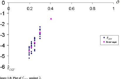
n= ... 42 Table 1-31: Relationship between 2

η

σ and δ ... 43 Table 1-32: Power of SIMEX-based test using _{a b+ δ}c_{as the extrapolating function}

(

2 _0.1,0.2,0.3

)

η

σ = , 100n= ... 47 Table 1-33: Power of SIMEX-based test using _{a b+ δ}c_{as the extrapolating function}

(

2 _0.4,0.5,0.6

)

η

σ = , 100n= ... 47 Table 1-34: Power of SIMEX-based test using _{a b+ δ}c_{as the extrapolating function}

(

2 _0.7,0.8,0.9

)

η

σ = , 100n= ... 47 Table 1-35: Power of SIMEX-based test using _{a b+ δ}c_{as the extrapolating function}

(

2 _{1, 2,3}

)

η

σ = , 100n= ... 48 Table 1-36: Power of SIMEX-based test using _{a b+ δ}c_{as the extrapolating function}

(

2 _4,5,10

)

η

σ = , 100n= ... 48 Table 1-37: Power of SIMEX-based test using _{a b+ δ}c_{as the extrapolating function}

(

2 _50,100

)

η

σ = , 100n= ... 48 Table 1-38: Performance of _{a b+ δ}1.2_{for different values of 2}

1

η

σ ≥ , 100n= ... 49 Table 1-39: Performance of _{a b+ δ}1.2_{for different values of 2}

1

η

σ < , 100n= ... 50 Table 1-40: Power of SIMEX-based test using _{a b}ˆc

λ

δ

+ as extrapolating function

(

2 _0.1,0.2,0.3

)

η

σ = , 100n= ... 51 Table 1-41: Power of SIMEX-based test using _{a b}ˆc

λ

δ

+ as extrapolating function

(

2 _0.4,0.5,0.6

)

η

σ = , 100n= ... 52 Table 1-42: Power of SIMEX-based test using _{a b}ˆc

λ

δ

+ as extrapolating function

(

2 _{0.7,0.8,0.9,1}

)

η

σ = , 100n= ... 52 Table 1-43: Power of SIMEX-based test using _{a b}ˆc

λ

δ

+ as extrapolating function

(

2 _2,3

)

η

Table 1-44: Power of SIMEX-based test using _{a b}ˆc

λ

δ

+ as extrapolating function

(

2 _4,5,8

)

η

σ = , 100n= ... 53

Table 1-45: Power of SIMEX-based test using _{a b}ˆc λ δ + as extrapolating function

(

2 _10,100

)

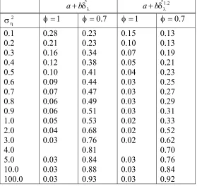
η σ = , 100n= ... 53

Table 1-46: Comparing a b+ δˆ_λ and _{a b}ˆ1.2 λ δ + as extrapolating functions, n=100... 54

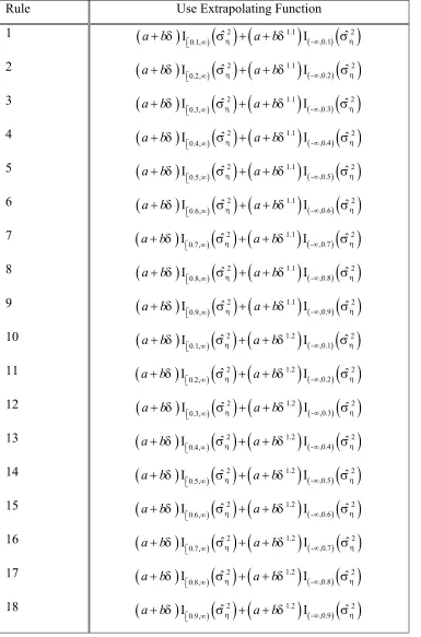
Table 1-47: Different rules for combining the extrapolating functions a b+ δˆ_λ and 1.2 ˆ a b+ δ_λ ... 56

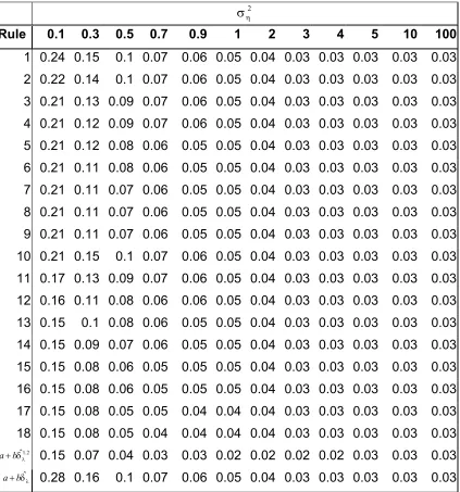
Table 1-48: Estimated size of the SIMEX test using different rules , n=100 ... 58

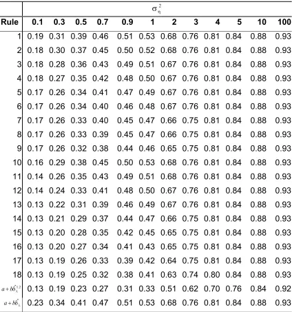
Table 1-49: Estimated power of the SIMEX test using different rules at H₁:φ =0.7, 100 n= ... 59

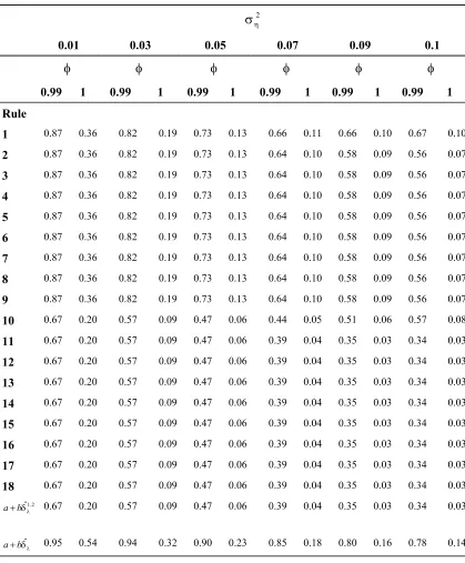
Table 1-50: Power and Size of various rules when Sample Size n=1000 and 2 0.01≤σ_η ≤0.10... 60

Table 2-1: Percentiles from the Simulated distribution of τ ... 64

Table 2-2: Power Comparison for n=25 ... 65

Table 2-3: Power Comparison for n=100... 65

Table 2-4: Power Comparison for n=1000... 65

Table 2-5: Asymptotic Percentiles of τ ... 72

Table 2-6: Size and Power based on Finite Sample Percentiles under various specifications for the Error distribution ... 78

Table 2-7: Size and Power based on Asymptotic Percentiles under various specifications for the Error distribution ... 79

Table 2-8: Size and Power based on Finite Sample Percentiles under centered Skew-Normal, Skew-t, Uniform and Exponential distributions. ... 80

Table 2-9: Size and Power based on Asymptotic Percentiles under centered Skew-Normal, Skew-t, Uniform and Exponential distributions. ... 81

Table 2-10: Rejection Probabilities when e_t ~

{

Exponential

( )

1 -1 or

}

Uniform

(

−0.5,0.5

)

, 25 n= based on asymptotic percentiles... 82

Table 2-11: Rejection Probabilities when e_t ~

{

Exponential

( )

1 -1 or

}

Uniform

(

−0.5,0.5

)

, based on finite sample (n=25) percentiles... 82

Table 2-12: Rejection Probabilities when e_t ~

{

Exponential

( )

1 -1 or

}

Uniform

(

−0.5,0.5

)

, 50 n= based on asymptotic percentiles... 82

Table 2-13: Rejection Probabilities when e_t ~

{

Exponential

( )

1 -1 or

}

Uniform

(

−0.5,0.5

)

, based on finite sample (n=50) percentiles... 83

Table 2-14: Rejection probabilities when the error distribution is given by the cone-shaped distribution (2.5.1) and the sample size n=50 ... 84

Table 2-15: Rejection probabilities when the error distribution is given by the cone-shaped distribution (2.5.1) and the sample size n=25 ... 84

Table 3-1: 95th percentile based on OLS statistic (2) , OLS n τ ... 93

Table 3-3: 95th percentile based on OLS statistic (1) ,

WS n

τ ... 94

Table 3-4: 5th _{percentile based on OLS statistic} (2) , WS n τ ... 95

Table 3-5: Size and Power of the IUT based on OLS, n=100... 97

Table 3-6: Size and Power of IUT based on OLS, n=500 ... 97

Table 3-7: Size and Power based of IUT based on OLS, n=1000 ... 97

Table 3-8: Size and Power based on WS statistic, n=100... 98

Table 3-9: Size and Power based on WS statistic, n=500 ... 99

Table 3-10: Size and Power based on WS statistic, n=1000... 99

Table 3-11: Asymptotic Percentiles corresponding to various values of γ ... 101

Table 3-12: Rejection probabilities under the null and alternative hypothesis based on asymptotic percentiles... 102

Table 3-13: Size and Power of TS1 for seven different DC and three different sample sizes... 105

Table 3-14: Size and Power of TS2 for seven different DC and three different sample sizes... 105

Table 3-15: Size and Power of TS3 for seven different DC and three different sample sizes... 106

Table 3-16: Size and Power of TS4 for seven different DC and three different sample sizes... 106

Table 3-17: Size and Power of TS5 for seven different DC and three different sample sizes... 106

Table 3-18: 95th percentile based on the distribution of (1) , OLS n τ ... 108

Table 3-19: 5th percentile based on the distribution of (2) , OLS n τ ... 109

Table 3-20: 95th percentile based on the distribution of (1) , ws n τ ... 109

Table 3-21: 5th percentile based on the distribution of (2) , ws n τ ... 109

Table 3-22: Size and Power of the IUT based on (1) , OLS n τ and (2) , OLS n τ , 100n= ... 111

Table 3-23: Size and Power of the IUT based on (1) , OLS n τ and (2) , OLS n τ , 500n= ... 111

List of Figures

Figure 1-1: Linear extrapolating function a b+ λ ... 15

Figure 1-2: A quadratic extrapolating function _{a b+ λ+cλ}2 _{... 16}

Figure 1-3: The extrapolating function a b+

(

λ+2

)

... 16

Figure 1-4: (a) Sample Plot of Z_{b IV,} ( )λ against λ ... 33

Figure 1-5: (b) Sample Plot of Z_{b IV,} ( )λ against λ ... 33

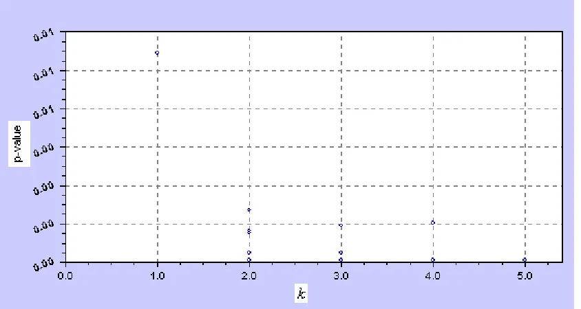
Figure 1-6: (a) Plot of p-values against : # of measurement errorsk ... 36

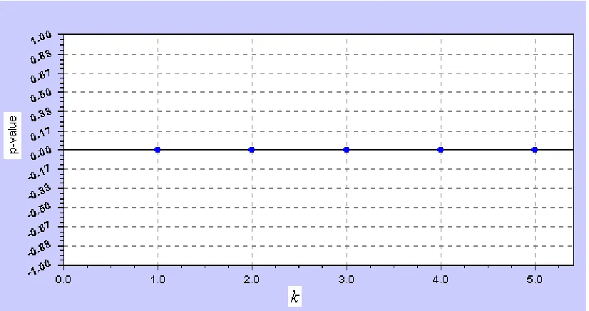
Figure 1-7: (b) Plot of p-values against : # of measurement errorsk ... 38

Figure 1-8: Plot of ˆτ_OLS against λ... 45

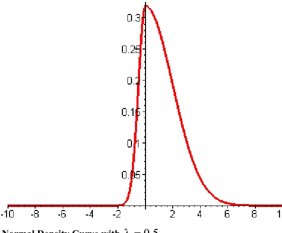
Figure 2-1:Skew-Normal Density Curve with λ =0.5 ... 73

Figure 2-2: Skew-Normal Density with λ =1.5 ... 74

Figure 2-3: Skew t-distribution with 10 d.f. and λ =1... 74

Figure 2-4: Skew-t distribution with 10 d.f. and λ =0.5... 75

Figure 2-5: Skew-t distribution with 10 d.f. and λ =1.5 ... 75

Chapter 1 SIMEX -BASED UNIT ROOT

TEST FOR STOCHASTIC

VOLATILITY MODELS

Section 1. Introduction

Modeling the volatility of the price of an asset is central to the determination of the price of various financial instruments. Engle (1982) proposed the Autoregressive Conditional Heteroskedasticity (ARCH) models to analyze economic times series. In the ARCH models, the conditional variance of the white noise process is allowed to change over time. This aspect of time-dependent conditional variance is the consequence of modeling the square of the white noise error process as an Autoregressive (AR) process. The lack of parsimonious ARCH models led to the development of generalized autoregressive conditionally heteroscedastic (GARCH) models. Bollerslev (1986) proposed the GARCH models that model the square of the white noise process as an Autoregressive Moving Average (ARMA) process.

Stochastic Volatility Model (SVM) serves as an alternative to ARCH and GARCH models. Taylor (1982) introduced the first discrete-time SVM in which the observed time series is expressed in terms of an unobserved variance component and an independent and identically distributed (i.i.d.) error.

Let r_t be an observed time series (e.g. stock returns). Then we consider the following SVM for r_t:

(

)

1

exp 2 ,

( ) ( ) , 1,..., ,

t t t

t t t

r u h

h µ φ h₋ µ η t n

=

where u_t and η_t are zero-mean white noise with variance 1 and 2

η

σ , respectively. Also,

t

u and η_t are assumed to be stochastically independent.

Equation (1.1.1) shows that the unobserved variance component h_t has been modeled as an autoregressive process with mean µand AR parameter φ.

In equation (1.1.1), if φ=1 then the SVM is non-stationary (unit root process) and volatility is said to be persistent. On the other hand, if the magnitude of φ is less than one, the volatility is said to be transient in nature implying that the effect of a shock on the future volatility will eventually die out.

So, Lam and Li (1997) addressed the issue of persistence of volatility in seven Southeast Asian markets, by the SVM defined in (1.1.1). They concluded that the shocks to volatility are transient in the whole period (1980-91) in all the seven Southeast Asian indices. A Bayesian approach to testing for a unit-root in SVM was proposed by So and Li (1999). They applied their method to the seven indices of So et al. (1997) and the S & P 500 data. Their method leads to slightly different results as compared with the ADF tests. The null hypothesis of nonstationarity is rejected in all cases according to the classical test. Using the posterior odds ratio, they found strong evidence favoring stationary volatility for most of the market indices they considered.

In this paper, we focus on unit root tests for the volatility process based on a frequentist approach. The stochastic volatility model implies that the log of the squared time series, i.e., _{log( )}2

t

r is an ARMA (1,1) process with the autoregressive root being the same as the autoregressive root of the volatility process h_t. One may test for a unit root in the unobserved volatility process h_t by testing for a unit root in the log of the squared time series _{log( )}2

t

r . Unfortunately, for small values of 2

η

σ , the MA parameter in _{log( )}2

t

r

process has a large negative moving average root and the standard unit root tests are known to suffer from extreme size distortions in the presence of negative MA roots as shown in Pantula (1991). Because the standard unit root tests reject the null hypothesis of a unit root too often when the moving average parameter is very close to one, they are unreliable. In this paper, our goal is to investigate whether the procedure of testing for a unit root in the _{log( )}2

t

r process based on ordinary least squares (OLS), weighted symmetric estimators (WS) and instrumental variables (IV) can be modified to obtain test procedures which maintain the correct level of significance and still deliver enough power to differentiate between the stationary and non-stationary series. Towards that end, we view model (1.1.1) as a model with measurement error. On taking logarithms on both sides of the representation of 2

t

r in (1.1.1), we get _{log( )}2 _{log( )}2

t t t

r = +h u . Note that the observed data _{log( )}2

t

the error _{log( )}2

t

u (in the measurement of _{log( )}2

t

r ). The regression model is given by the second equation in (1.1.1), (h_t −µ)=φ(h_t−1−µ η)+ _t.

Cook and Stefanski (1994) developed the Simulation–Extrapolation (SIMEX) procedure in response to the need for fitting nonstandard, generalized linear measurement error models. It is a simulation-based method of estimating and reducing bias due to measurement error. In this method, estimates are obtained by adding additional measurement error to the data, identifying a trend in the measurement error-induced statistic and extrapolating this trend back to the case of no measurement error. In this article, we investigate SIMEX-based procedures for testing H₀:φ =1against H₁:φ <1.

The remainder of the article is organized into seven sections. The next section discusses the application of the standard unit root tests to the volatility process and presents two estimation methods used by several of these tests. Section 3 describes the SIMEX procedure and how it can be used to derive a unit root test for the SVM. Section 4 presents an alternative way to generate the pseudo-errors in the SIMEX procedure. Section 5 presents the IV-based unit root test and the ADF test and compares their performance with the SIMEX-based test. Section 6 explores the applicability of the SIMEX method to the IV estimator. In Section 7, an attempt is made to apply the SIMEX procedure to the p-values instead of the test statistic values. Section 8 draws insight from asymptotic theory of OLS and WS estimators in ARMA models to specify an extrapolating function that would be valid irrespective of the value of 2

η

σ . In practice, the value of 2

η

σ will seldom be known and so Section 9 attempts to validate the SIMEX-based test in situations that require the estimation of 2

η

σ . To optimize the size and power performance of the SIMEX-based test, the simulation results of Section 9 suggest the use of different extrapolating functions depending on whether 2

η

σ is less than 1 or not. Section 10 seeks to address this issue by evaluating different rules of selecting an extrapolating function based on an estimate of 2

η

Section 2. Standard unit root tests for volatility

Note that on taking logarithm on both sides of the first equation in (1.1.1), we get,

2 2

log( )r_t = +h_t log( )u_t . It follows that _{log( )}2

t

r has the same covariance structure as that of a stationary ARMA(1, 1) process,

2 2

1 1

(log( )r_t −µ)=φ(log(r_t− )−µ)+ −ε θε_{t t−} ,φ <1. (1.2.1) But if φ =1, _{log( )}2

t

r is an ARIMA(0,1,1) process,

2 2

1 1

(log( )r_t −µ) (log(= r_t− )−µ)+ −ε θε_{t t−}, (1.2.2) where the ε_t’s are white noise with variance _σ2_{. If we let log( )}2

t t

e = u , then the mean and the variance of e_t are known to be approximately –1.2704 and _π2 _{2 respectively;}

see Abramovitz & Stegun (1970, Pg 943). We can compute the values of the parameters

θ and _σ2 _{in the model (1.2.2) by solving the equations} 2

2 2

2 2 2 and .

1 2

e

e e η

σ

θ _{θσ σ}

θ σ σ

−

= =

+ + (1.2.3)

Based on the ARMA representation in (1.2.1), we may use any one of the unit root tests available in the literature to test for a unit root in _{log( )}2

t

We now present two pivotal test statistics associated with two different kinds of estimators that exist in the literature for testing the null hypothesis H₀:φ =1, against the alternative hypothesis H_a:φ <1 in the AR model

(

)

2

1 , 0 0, ~ (0, ).

t t t t

Y − =µ φ Y₋ −µ +ε Y = ε NID σ (1.2.4)

The following two statistics are not appropriate for testing the hypothesis of nonstationarity in the _{log( )}2

t

r process because _{log( )}2

t

r follows an ARMA structure. But we present them to serve two purposes. The first purpose is to illustrate the size distortion of such tests when the ARMA(1,1) model is incorrectly specified to be a first-order AR process. The second purpose is to show, in a later section, how the SIMEX method applied to these statistics, controls the size distortion.

1. The ordinary least squares (OLS) statistic τˆ_OLS

It follows from equation (1.2.4) that Y_t =µ(1− +φ) φY_t−1+ =ε_t θ₀+φY_t−1+ε_t where

0 (1 )

θ =µ −φ . The regression t statistic for testing that the coefficient of Y_t−1 is 1 in the regression of Y_t on ‘1’ and Y_t−1 is,

1 2

1 2

1 1

2

ˆ

ˆ_OLS n _t ( 1),

t

s y

τ − φ

− =

 

= _{ } −



∑

 (1.2.5)

where

2 1 2

1 1

2

ˆ

( 2) n ( _{t t} )

t

s n − y φy

− =

= −

∑

−

and

1 2

1 1

2 2

ˆ n n

t t t t t

y y y

φ

−

− −

= =

 

=  

and

1

1 , n

t t t

t

y Y y y Y

n =

= − =

∑

2. The weighted symmetric (WS) statistic τˆ_ws

The WS estimator is a member of the class of symmetric estimators—the symmetry referring to the fact that if a normal stationary AR process satisfies (1.2.4), then it also

satisfies the equation

(

)

2

1 , ~ (0, )

t t t t

Y µ φ Y µ ε∗ ε∗ NID σ

+

− = − + . The WS estimator of φ,

given by

1 2 1

2 1 2

2 1

ˆ _,

n t t t

ws n n t t t t

y y

y n y

φ = − − − = = = +

∑

∑

∑

(1.2.6)

was studied by Park and Fuller (1993). It is obtained by minimizing

1

2 2

1 1 1

2 1

( ) n ( ) n (1 )( )

w t t t t t t

t t

Q φ w y φy₋ − w₊ y φy₊

= =

=

∑

− +

∑

− − , where 1_{( 1)}

t

w =n t− − , 2,3,...,t= n,

t t

y = −Y yand 1 1

n t t

y n− Y

=

=

∑

.

The pivotal statistic corresponding to ˆφ_ws is given by

1/ 2 1

2 1 2 1

2 1

ˆ

ˆ_{ws ws} 1 ,n _t n _t ˆ_ws

t t

y n y

τ φ − − σ−

= =

 

 

=_ − _ + _

 

∑

∑

 (1.2.7)

where

2 1 ˆ

ˆ_ws (n 2) Q_w( _ws)

σ _{= −} − φ _(1.2.8)

Monte Carlo study

2 2

1

log( ) log( )

( ) ( ) , 1,..., ,

t t t

t t t

r h u

h µ φ h₋ µ η t n

= +

− = − + = (1.2.9)

where u_t and η_t are zero-mean white noise with variance 1 and 2

η

σ , respectively. Also,

t

u and η_t are assumed to be stochastically independent.

We let h₀ =0 and µ =0. The RANNOR function in SAS (V8) was used to generate the

t

η ’s as independent standard normal variables ( 2 ₁

η

σ = ). The same function was used again to generate the u_t’s as independent standard normal variables independent of theη_t’s. We generated samples of size n=100 with φ =0.8,0.85,0.9,0.95,0.98. The two statistics ˆτ_OLS and ˆτ_wswere then computed by plugging in _{log( )}2

t t

Y = r in each of the expressions (1.2.5) and (1.2.7).

The finite sample (n=100) critical values (for a 5%-level test of H₀:φ =1 against

: 1

a

H φ < when the true process follows the AR model (1.2.4), are computed to be –2.90 and -2.55 (Tables 10.A.2 and 10.A.4 in Fuller (1996)) for ˆτ_OLS and ˆτ_ws respectively. These are the critical values that we used to test H₀:φ =1 against H_a:φ <1in the ARMA model for _{log( )}2

t

Table 1-1: P

(

τˆ_OLS < −2.90φ φ= ₀

)

and P

(

τˆ_WS < −2.55φ φ= ₀

)

, n=100

0

φ

Test Statistic _{1 0.98 0.95 0.90 0.85 0.80}

ˆ_OLS

τ 0.76 0.91 0.97 0.99 1.00 1.00

ˆ_WS

τ 0.80 0.95 0.99 0.99 1.00 1.00

As is evident from Table 1, both the OLS and the WS statistics have severe size distortions. More specifically, the WS statistic wrongly rejects the null hypothesis of nonstationarity more often than the OLS statistic does. Hence these tests are not reliable even though they produce high power at values of φ very close to 1.

For the above simulations, 2 ₁

η

σ = and 2 2 ₂

e

σ =π . Using equations (1.2.3), we get 0.6399

θ = − (we use the value of θ that is less than 1 in absolute value so that we have an invertible process) and _{σ =}2 _{7.71183. As shown in Pantula (1991), such size}

distortions become worse as the moving average parameter θ in the ARMA model (1.2.2) becomes closer to 1.

Section 3. Applying the SIMEX method to test the unit root hypothesis

measurement error modeling. We will first present the SIMEX procedure in a formal setting and then show how our model (1.2.9) can be fitted into the SIMEX framework. We will borrow heavily from Cook and Stefanski (1994) to formally describe the SIMEX method.

Let , , Y V U and Xdenote the response variable, a covariate measured without error, the true predictor, and the measured predictor. Assume that the true predictor and the measured predictor are related by the following equation:

X U= +σZ

where Z is a standard normal random variable independent of , and U V X and _σ2_{is the}

known measurement error variance. Suppose that the observed data is given by

1

{ , , }n i i i

Y V X .

Let

1

ˆ ({ , , } )n

true T Y V Ui i i

τ =

be an estimator of the parameter τ . ˆτ_true is not an estimator in the strict sense since it depends on the unknown { }₁n

i

U . But it is useful to have a notation for the random quantity.

For 0λ ≥ , define

1 2

,( ) ,,

b i i b i

X λ =X +λ σZ

where { _{, 1}}n b i

Z are mutually independent, independent of { , , , }₁n i i i i

Y V U X and identically distributed standard normal random variables. Define

, 1

ˆ ( ) ({ , , ( )})n b T Y V Xi i b i

τ λ = λ

and

1

ˆ( ) ( ( ) { , ,ˆ } );n b i i i

E Y V X

τ λ = τ λ

The expectation above is with respect to the distribution of { _{, 1}}n b i

Exact determination of ˆ( )τ λ for λ >0 is generally not feasible, but it can always be estimated arbitrarily well by generating a large number of independent measurement error vectors, {{ _,} }n₁ B₁

b i i b

Z _{= =} , computing ˆ ( )τ λ_b for b=1,...,B, and approximating ˆ( )τ λ by the sample mean of { ( )}ˆ ₁B

b

τ λ . { _,}n₁ b i i

Z ₌ are called pseudo-errors. This is the simulation component of the SIMEX method.

The extrapolation part of the method comprises modeling ˆ( )τ λ as a function of λ for 0

λ ≥ and using the model to extrapolate back to λ = −1. This yields the simulation extrapolation estimator, denoted by ˆτ_SIMEX. Here, λ = −1 corresponds to no measurement error in the model.

Assuming that ˆτ_true, ˆ ( )τ λ_b and ˆ( )τ λ have finite expectations and that a weak law of large number applies, each statistic converges in probability to its expectation. One can regard

ˆ ( ( ))_b

E τ λ to be a function of the true estimand τ₀ and the variance of the total

measurement error in X_i( )λ ; that is 2

,

( _{i b i}) (1 )

Var Z +σ λZ =σ +λ . If we denote this

function by 2

0

( , (1 ))

T τ σ +λ , then ˆ ( )τ λ_b converges in probability to 2 0

( , (1 ))

T τ σ +λ . Also, if _{σ =}2 _{0(i.e., if there is no measurement error), then ˆ}

true

τ = ˆ ( )τ λ_b = ˆ( )τ λ (almost surely). So if ˆτ_true is a consistent estimator of τ₀, then τ₀ =T( ,0)τ₀ . Now, provided

(.,.)

T is a continuous function, we are also led to the conclusion that

2

0 0 0

1 ˆ 1 ˆ 1

lim ( ( )) lim ( ( )) lim ( ,E E _b T (1 )) T( ,0) λ→− τ λ =λ→− τ λ =λ→− τ σ +λ = τ =τ .

Thus the extrapolation of the fitted model to λ = −1, which is ˆτ_SIMEX, is an approximately consistent estimator of τ₀. The SIMEX estimator is only approximately consistent in general, because the estimated extrapolation function is generally an approximation.

2 2

2

ln log( )

( ( 1.27)) (log( ) ( 1.27))

t t t

t t

t t

r h u

h u

h∗ e

= +

= + − + − −

= +

where _(ln 2_{) 1.27}

t

E u = − and _ln 2 _1.27

t t

e = u + are independent _log(χ2_{)variables with}

mean zero and variance _π2 _2.

So h_t∗_{can be viewed as the true variate subject to measurement error,}

t

e , and _{log( )}2

t

r

can be looked upon as the measurement of h_t∗_{. Let log( )}2

t t

Y = r . Then Y_t is an ARMA(1,1) process satisfying (1) (1) (1)

1 1

t t t t

Y =Y₋ +ε −θ ε₋ , (1)

t

ε being white noise with variance (1)

2 ε σ . Define 1 1

, n

t t t

t

h h h h n− h

= ′ = − =

∑

1/ 2 2 1 2 1/ 2 1

2 1 2 1

2 1

ˆ ₁

ˆ

ˆ

ˆ

ˆ 1 ˆ

n OLS OLS t t OLS n n

ws ws t t ws t t

h

h n h

φ τ σ τ φ σ − = − − − = = −  _′  = _{ }       ′ ′ =_ − _ + _   

∑

∑

∑

where 1 2 1 1 2 2

2 1 2

1 2

1 2 1

2 1 2

2 1

ˆ

ˆ

ˆ ( 2) ( )

ˆ

n n OLS t t t

t t n

OLS t OLS t t

n t t t

ws n n t t t t

h h h

n h h

h h

h n h

2 1

1

2 2

1 1 1

2 1

ˆ

ˆ ( 2) ( )

( ) ( ) (1 )( ) .

ws w ws

n n

w t t t t t t

t t

n Q

Q w h h w h h

σ φ φ φ φ − − − + + = = = − ′ ′ ′ ′ =

∑

− +

∑

− − ˆ_OLS

τ and ˆτ_WS are the OLS and WS statistics respectively based on the unknown { }₁n t

h . They are akin to the ˆτ_true estimator defined above in the description of the SIMEX procedure. Next, we define

,( ) ,, 0

1, 2,..,

b t t b t

Y Y e

b B

λ = + λ λ>

= (1.3.1)

where e_{b t,} are independent _log(χ2_{)variables with mean zero and variance π}2 _2.

Just as we had defined ˆ ( )τ λ_b above, similarly we define

1 2

, 2

, , 1

2 ,

ˆ _{( ) 1}

ˆ ( ) ( )

ˆ

n b OLS

b OLS b t t b OLS y φ λ τ λ λ σ − = −   = _{ }



∑

 (1.3.2)

and

1/ 2 1

2 1 2 1

, , , , ,

2 1

ˆ

ˆ_{b ws}( ) _{b ws}( ) 1 ( )n _{b t} n _{b t}( ) ˆ_{b ws}

t t

y n y

τ λ φ λ − λ − λ σ−

= =

 

 

=_ − _ + _

 

∑

∑

 (1.3.3)

where φˆ_{b OLS,} ( )λ , φˆ_{b WS,} ( )λ , σˆ_{b OLS,} and 1 ,

ˆ_{b ws}

σ− _{are now based on}

,( ) ,( ) , ( )

b t b t b t

y λ =Y λ −Y λ

and 1

, ,

1

( ) n ( )

b t b t t

Y λ n− Y λ

=

For 0λ > , we can generate a large number of independent pseudo-errors {{ } }_, n₁ B₁ b t t b

e _{= =} and compute τˆ_{b OLS,} ( )λ and τˆ_{b ws,} ( )λ for b=1, 2,...,B. The final step of the SIMEX method calls for modeling τˆ_{b OLS,} ( )λ and τˆ_{b ws,} ( )λ as functions of λ for λ ≥0 and using the model to extrapolate back to λ = −1. This yields τˆ_{SIMXEX OLS,} and τˆ_{SIMXEX ws,} as estimates of

ˆ_OLS

τ and ˆτ_ws respectively. We can now compare τˆ_{SIMXEX OLS,} and τˆ_{SIMXEX ws,} with the percentiles given in Fuller (1996), for ˆτ_µ and ˆτ_w respectively to either reject or fail to reject H₀:φ =1.

Monte Carlo Study:

In this simulation study, we again set h₀ =0 andµ =0 in the model (1.2.9). The η_t’s are generated as independent standard normal variables using the RANNOR function in SAS (V8). To generate 'e s_t as independent _log(χ2_{)variables with mean zero and variance}

2 ₂

π , the u_t’s were first generated as independent standard normal variables independent of the η_t’s and then the value 1.2704 was subtracted from the log of the

square of each u_t. We generated samples of size n=100 with

0.8,0.85,0.9,0.95,0.98,1

φ = . The two statistics ˆτ_µ and ˆτ_ws were then computed from the expressions (1.2.5) and (1.2.7) respectively. Note that so far, we have just computed what we would usually compute when using the standard unit root test (based on OLS and WS) on the _ln 2

t

r process.

The next step is the simulation-step of the SIMEX method. The e_{b t,} ’s for each b were generated as independent _log(χ2_{)variables with mean zero and variance π}2 _{2 in the}

same way as the e_t’s were generated. For λ =0.5,1.5, 2.5 and 3.5, we then generated samples of size 100 on the variables 10

, 1

{Y_{b t}( )}λ _b= using equation (1.3.1) and computed

10

, 1

ˆ

{τ_{b OLS}( )}λ _b= and 10

, 1

ˆ

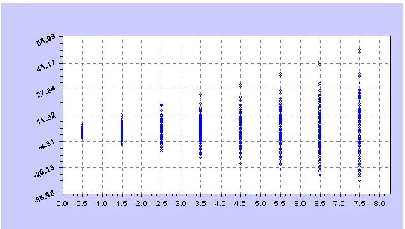
Figure 1-1: Linear extrapolating function a b+ λ

The extrapolation step of the SIMEX method required some preliminary investigation. We set φ =1 and performed a few replications of the entire procedure described in the previous two paragraphs and plotted 10

, 1

ˆ

{τ_{b OLS}( )}λ _b= and 10

, 1

ˆ

{τ_{b ws}( )}λ _b= against λ. Figure 1-1 and Figure 1-2 show the fit of the linear (a b+ λ) and quadratic fit (_{a b+ λ+cλ}2_{) to a}

representative plot of 10

, 1

ˆ

{τ_{b OLS}( )}λ _b= . Figure 1-3 shows the fit of the curve, a b+ (λ+2) to the same plot. Note that the lone value plotted at λ =0 corresponds to the statistic for

2

log( )

t t

Figure 1-2: A quadratic extrapolating function a b+ λ+cλ2

Figure 1-3: The extrapolating function a b+

(

λ+2

)

proportion of times the null hypothesis H₀:φ =1 was rejected and (b) the proportion of times the null hypothesis of no lack-of-fit was rejected for each of the three regression models, when the data was generated using φ =0.8,0.85,0.9,0.95,0.98,1.

Regression curves similar to the ones obtained in figures 1, 2 and 3, were also obtained

for 10

, 1

ˆ

{τ_{b ws}( )}λ _b= . Again, all the three regression models were applied and in each case,

,

ˆ_{b ws}( )

τ λ was extrapolated at λ = −1. The null hypothesis H₀:φ =1 was rejected if the extrapolated value was less than –2.55.

From the following tables of simulated power computations and Lack-of-fit tests, we observe that the results for the OLS estimator are very much similar to those for the WS estimator. When 2 ₁

η

σ = , the regression function a b+ (λ+2) provides the best fit to the OLS and the WS statistic for any value of φ and also maintains the size close to the nominal significance level of 0.05. While in the OLS case, the simulated size falls within

3σ limits,

(

0.05 3 0.05 0.95 5000,0.05 3 0.05 0.95 5000− ∗ + ∗

)

= (0.041, 0.059) of 0.05, the simulated size in the WS case is 0.063, slightly above the upper 3σ limit, 0.059.

As we let 2

η

σ assume larger values, the fit of the regression function

( 2)

a b+ λ+ deteriorates for values of φ, closer to 1. The simulated size of the test using this regression function also falls well below the lower 3σ limit, 0.041. In contrast to the performance of the inverse linear relationship, the performance of the linear and the quadratic polynomials improve as 2

η

σ increases from 1 to 10. When 2 _1.5

η

σ = or 2 ₂

η

σ = , none of the regression functions considered here yield a size close to the nominal size, 0.05. On one hand, the linear polynomial function delivers a rejection rate that is too high under the unit root null hypothesis to produce a reliable test and on the other hand, the inverse linear function, a b+ (λ+2) delivers a rejection rate that is too low to produce a test with sufficient power. The quadratic polynomial provides the best fit to the OLS and the WS statistics when 2 ₂

η

Table 1-2: P

(

τˆ_{SIMEX OLS,} < −2.90φ φ= ₀

)

when σ =_η2 1, n=100

0

φ

Regression 0.70 0.80 0.85 0.90 0.93 0.95 0.98 1.00

a b+ λ 1.000 1.000 1.000 0.997 0.982 0.957 0.874 0.690

Lack-of-fit 0.027 0.035 0.042 0.050 0.036 0.057 0.053 0.048

2

a b+ λ+cλ 0.996 0.983 0.955 0.881 0.798 0.716 0.567 0.400

Lack-of-fit 0.061 0.078 0.090 0.105 0.113 0.118 0.114 0.101

( 2)

a b+ λ+ 0.640 0.467 0.354 0.232 0.168 0.129 0.081 0.051

Lack-of-fit 0.000 0.000 0.000 0.000 0.000 0.000 0.000 0.002

Table 1-3: P

(

τˆ_{SIMEX OLS,} < −2.90φ φ= ₀

)

when σ =_η2 1.5, n=100

0

φ

Regression 0.70 0.80 0.85 0.90 0.93 0.95 0.98 1.00

a b+ λ 1.000 1.000 0.997 0.976 0.928 0.869 0.728 0.522

Lack-of-fit 0.039 0.047 0.053 0.058 0.060 0.060 0.054 0.0428

2

a b+ λ+cλ 0.986 0.935 0.854 0.714 0.600 0.503 0.358 0.235

Lack-of-fit 0.087 0.109 0.152 0.126 0.126 0.125 0.113 0.096

( 2)

a b+ λ+ 0.396 0.226 0.154 0.083 0.054 0.037 0.023 0.014

Lack-of-fit 0.000 0.000 0.000 0.000 0.000 0.001 0.001 0.005

Table 1-4: P

(

τˆ_{SIMEX OLS,} < −2.90φ φ= ₀

)

when σ =_η2 2, n=100

0

φ

Regression 0.70 0.80 0.85 0.90 0.93 0.95 0.98 1.00

a b+ λ 1.000 0.998 0.986 0.935 0.846 0.759 0.585 0.393

Lack-of-fit 0.045 0.053 0.054 0.060 0.060 0.055 0.049 0.038

2

a b+ λ+cλ 0.963 0.852 0.735 0.562 0.441 0.350 0.231 0.149

Lack-of-fit 0.103 0.121 0.127 0.127 0.125 0.123 0.107 0.086

( 2)

a b+ λ+ 0.239 0.113 0.065 0.033 0.020 0.014 0.008 0.005

If we set 2 ₁₀

η

σ = , the empirical size obtained by employing the first-degree polynomial in

λ is 0.035—still falls outside the 3σ -interval but the test yields higher power than that obtained by the other two regression functions, at lower values of φ.

While the fit provided by the function a b+ λ to the OLS or the WS statistic when

2 ₁₀

η

σ = is not as good a fit as that provided by a b+ (λ+2) when 2 ₁

η

σ = , the power obtained by a b+ λ when 2 ₁₀

η

σ = is much higher than that obtained by

( 2)

a b+ λ+ when 2 ₁

η

σ = .

We also performed simulations by setting 2 _0.5

η

σ = , 0.1. For both these cases, although the fit provided by some of the regression functions considered are very good, the proportion of false rejections obtained at φ =1 is much larger than the nominal significance level.

Table 1-5: P

(

τˆ_{SIMEX OLS,} < −2.90φ φ= ₀

)

when σ =_η2 10, n=100

0

φ

Regression 0.70 0.80 0.85 0.90 0.93 0.95 0.98 1.00

a b+ λ 0.947 0.667 0.425 0.210 0.116 0.079 0.045 0.035

Lack-of-fit 0.009 0.008 0.007 0.006 0.004 0.005 0.006 0.007

2

a b+ λ+cλ 0.628 0.247 0.119 0.044 0.024 0.014 0.009 0.017

Lack-of-fit 0.023 0.021 0.021 0.018 0.017 0.017 0.014 0.017

( 2)

a b+ λ+ 0.002 0.000 0.000 0.000 0.000 0.000 0.000 0.000

Table 1-6: P

(

τˆ_{SIMEX OLS,} < −2.90φ φ= ₀

)

when σ =_η2 0.5, n=100

0

φ

Regression 0.7 1

a b+ λ 1.000 0.860

Lack-of-fit 0.009 0.060

2

a b+ λ+cλ 1.000 0.720

Lack-of-fit 0.021 0.082

( 2)

a b+ λ+ 0.896 0.200

Lack-of-fit 0.000 0.000

2

( 2)

a b+ λ+ 0.350 0.060

Lack-of-fit 0.000 0.000

Table 1-7: P

(

τˆ_{SIMEX OLS,} < −2.90φ φ= ₀

)

when σ =_η2 0.1, n=100

0

φ

Regression 0.70 1.00

a b+ λ 1.000 1.000

Lack-of-fit 0.000 0.000

2

a b+ λ+cλ 1.000 1.000

Lack-of-fit 0.000 0.010

( 2)

a b+ λ+ 1.000 0.849

Lack-of-fit 0.000 0.000

2

( 2)

a b+ λ+ 0.912 0.456

Lack-of-fit 0.000 0.000

The following tables report the power of the SIMEX test based on the WS estimator and the results of the lack-of-fit test on the basis of 5000 replications, for various values of

2

η

Table 1-8: P

(

τˆ_{SIMEX WS,} < −2.55φ φ= ₀

)

when σ =_η2 1, n=100

0

φ

Regression 0.70 0.80 0.85 0.90 0.93 0.95 0.98 1.00

a b+ λ 1.000 1.000 1.000 0.986 0.981 0.972 0.845 0.673

Lack-of-fit 0.022 0.023 0.040 0.051 0.052 0.059 0.057 0.046

2

a b+ λ+cλ 0.992 0.989 0.945 0.865 0.801 0.742 0.543 0.367

Lack-of-fit 0.071 0.071 0.104 0.104 0.111 0.118 0.122 0.101

( 2)

a b+ λ+ 0.766 0.579 0.451 0.310 0.223 0.170 0.102 0.063

Lack-of-fit 0.000 0.000 0.000 0.000 0.000 0.000 0.000 0.001

Table 1-9: P

(

τˆ_{SIMEX WS,} < −2.55φ φ= ₀

)

when σ =_η2 1.5, n=100

0

φ

Regression 0.70 0.80 0.85 0.90 0.93 0.95 0.98 1.00

a b+ λ 1.000 1.000 1.000 0.986 0.900 0.896 0.706 0.542

Lack-of-fit 0.033 0.059 0.066 0.055 0.089 0.061 0.044 0.015

2

a b+ λ+cλ 0.956 0.922 0.841 0.722 0.615 0.509 0.351 0.237

Lack-of-fit 0.086 0.108 0.154 0.136 0.116 0.111 0.112 0.083

( 2)

a b+ λ+ 0.398 0.2522 0.156 0.088 0.054 0.040 0.012 0.015

Lack-of-fit 0.000 0.000 0.000 0.000 0.000 0.0010 0.001 0.005

Table 1-10: P

(

τˆ_{SIMEX WS,} < −2.55φ φ= ₀

)

when σ =_η2 2, n=100

0

φ

Regression 0.70 0.80 0.85 0.90 0.93 0.95 0.98 1.00

a b+ λ

1.000 0.998 0.956 0.932 0.880 0.746 0.555 0.336

Lack-of-fit _{0.043 0.052 0.054 0.063 0.065 0.055 0.048 0.039}

2

a b+ λ+cλ

0.950 0.851 0.715 0.587 0.492 0.356 0.200 0.160

Lack-of-fit

0.101 0.103 0.127 0.127 0.110 0.138 0.160 0.084

( 2)

a b+ λ+

0.225 0.135 0.066 0.032 0.022 0.014 0.005 0.005

Lack-of-fit

Table 1-11: P

(

τˆ_{SIMEX WS,} < −2.55φ φ= ₀

)

when σ =_η2 10, n=100

0

φ

Regression 0.70 0.80 0.85 0.90 0.93 0.95 0.98 1.00

a b+ λ

0.948 0.662 0.455 0.228 0.120 0.088 0.046 0.035

Lack-of-fit

0.009 0.008 0.007 0.006 0.004 0.004 0.005 0.007

2

a b+ λ+cλ

0.628 0.247 0.119 0.044 0.024 0.014 0.009 0.017

Lack-of-fit _{0.021 0.022 0.025 0.020 0.016 0.020 0.015 0.017}

( 2)

a b+ λ+ _{0.002 0.000 0.000 0.000 0.000 0.000 0.000 0.000}

Lack-of-fit

0.001 0.001 0.005 0.013 0.020 0.022 0.036 0.048

Table 1-12: P

(

τˆ_{SIMEX WS,} < −2.55φ φ= ₀

)

when σ =_η2 0.5, n=100

0

φ

Regression 0.70 1.00

a b+ λ _{1.00 0.89}

Lack-of-fit _{0.00 0.03}

2

a b+ λ+cλ _{1.00 0.77}

Lack-of-fit _{0.00 0.08}

( 2)

a b+ λ+ _{0.96 0.25}

Lack-of-fit _{0.00 0.00}

2

( 2)

a b+ λ+ 0.40 0.09

Table 1-13: P

(

τˆ_{SIMEX WS,} < −2.55φ φ= ₀

)

when σ =_η2 0.1, n=100

0

φ

Regression 0.70 1.00

a b+ λ _{1.00 1.00}

Lack-of-fit _{0.00 0.00}

2

a b+ λ+cλ _{1.00 1.00}

Lack-of-fit _{0.00 0.00}

( 2)

a b+ λ+ _{1.00 0.86}

Lack-of-fit _{0.00 0.00}

2

( 2)

a b+ λ+ 0.89 0.51

Lack-of-fit _{0.00 0.00}

Section 4. Performance of SIMEX-based test using a different mechanism to generate pseudo-errors

The method of adding additional measurement errors to the original data according to (1.3.1) can be slightly modified. We shall refer to the following procedure as the non-lambda approach in the later sections. Let us define (1) 2

, log( )

b t t

Y = r and subsequently the following:

( ) ( 1) ( )

, , , , 2,3,....

k k k b t b t b t

Y ₌Y − ₊e k_{= (1.4.1)}

where ( ) ,

k b t

e are independent _log(χ2_{)variables with mean zero and variance} 2

2

π _.

( ) ,k

b t

Y is the result of adding ‘k’additional independent measurement errors to *

t

h . Let us denote the OLS and the WS statistics based on ( )

,

k b t

Y by ( ) ,

ˆk b OLS

τ and ( ) ,

ˆk b ws

τ respectively, for 1, 2,...,

b= B. For k =2,3,..., we can generate a large number of independent pseudo-errors ( )

, 1 1

{{ k } }n B b t t b

e _{= =} and compute ( ) ,

ˆk b OLS

τ and ( )

,

ˆk b ws

τ for b=1, 2,...,B. Finally, ( ) ,

ˆk b OLS

τ and

( ) ,

ˆk b ws

τ can be modeled as functions of k for k =1, 2,3,... . To get the SIMEX estimators

,

ˆ_{SIMXEX OLS}

that the case k=0 corresponds to the unobserved *

t

h that is devoid of any measurement error. At the nominal significance level of 0.05, we compare τˆ_{SIMXEX OLS,} and τˆ_{SIMXEX ws,} with the percentiles –2.90 (for ˆτ_OLS) and –2.55 (for ˆτ_ws) respectively to either reject or fail to reject H₀:φ =1.

The power computations for the OLS and the WS estimators based on the above approach of genearting pseudo-errors, are given below. The results are very similar to the ones obtained in the previous section.

For 2 ₁

η

σ = , the regression function a b+ (1+k)provides the best fit to the OLS as well as the WS statistics. Again, the simulated size of 0.0558 in the case of OLS falls within the 3σ limits of the nominal size of 0.05. In the case of WS, the simulated size is 0.0652 which falls outside the 3σ limits of the nominal size of 0.05.

Table 1-14: P

(

τˆ_{SIMEX OLS,} < −2.90φ φ= ₀

)

when σ =_η2 1, n=100

0

φ

Regression 0.70 0.80 0.85 0.90 0.93 0.95 0.98 1.00

a bk+ 1.000 1.000 1.000 0.999 0.994 0.980 0.920 0.759

Lack-of-fit 0.021 0.031 0.037 0.044 0.047 0.049 0.050 0.046

2

a bk ck+ + 0.997 0.984 0.961 0.896 0.825 0.754 0.615 0.445

Lack-of-fit 0.062 0.075 0.086 0.103 0.108 0.114 0.115 0.105

(1 )

a b+ +k 0.636 0.471 0.364 0.253 0.181 0.141 0.083 0.056

Table 1-15: P

(

τˆ_{SIMEX OLS,} < −2.90φ φ= ₀

)

when σ =_η2 1.5, n=100

0

φ

Regression 0.70 0.80 0.85 0.90 0.93 0.95 0.98 1.00

a bk+ 1.000 1.000 0.999 0.991 0.965 0.921 0.803 0.602

Lack-of-fit 0.033 0.044 0.047 0.053 0.053 0.053 0.050 0.043

2

a bk ck+ + 0.986 0.939 0.879 0.754 0.650 0.562 0.413 0.277

Lack-of-fit _{0.079 0.010 0.109 0.121 0.125 0.127 0.119 0.101}

(1 )

a b+ +k _{0.415 0.251 0.167 0.096 0.065 0.048 0.026 0.015}

Lack-of-fit _{0.000 0.000 0.000 0.001 0.001 0.002 0.006 0.022}

Table 1-16: P

(

τˆ_{SIMEX OLS,} < −2.90φ φ= ₀

)

when σ =_η2 2, n=100

0

φ

Regression 0.70 0.80 0.85 0.90 0.93 0.95 0.98 1.00

a bk+ 1.000 0.999 0.997 0.969 0.912 0.840 0.681 0.474

Lack-of-fit 0.041 0.0482 0.051 0.052 0.052 0.050 0.048 0.043

2

a bk ck+ + 0.965 0.876 0.774 0.619 0.492 0.409 0.276 0.178

Lack-of-fit 0.094 0.111 0.120 0.128 0.129 0.126 0.113 0.094

(1 )

a b+ +k 0.257 0.125 0.079 0.039 0.022 0.015 0.010 0.006

Lack-of-fit 0.000 0.000 0.000 0.001 0.003 0.004 0.012 0.033

Table 1-17: P

(

τˆ_{SIMEX OLS,} < −2.90φ φ= ₀

)

when σ =_η2 10, n=100

0

φ

Regression 0.70 0.80 0.85 0.90 0.93 0.95 0.98 1.00

a bk+ 0.975 0.768 0.548 0.301 0.200 0.123 0.068 0.051

Lack-of-fit 0.011 0.014 0.015 0.014 0.013 0.012 0.011 0.0132

2

a bk ck+ + 0.665 0.306 0.159 0.066 0.041 0.023 0.015 0.019

Lack-of-fit 0.036 0.038 0.039 0.038 0.034 0.035 0.034 0.034

(1 )

a b+ +k 0.002 0.000 0.000 0.000 0.000 0.000 0.000 0.000

Table 1-18: P

(

τˆ_{SIMEX OLS,} < −2.90φ φ= ₀

)

when σ =_η2 0.5, n=100

0

φ

Regression 0.70 1.00

a bk+ 1.000 0.751

Lack-of-fit 0.000 0.050

2

a bk ck+ + 1.000 0.551

Lack-of-fit 0.000 0.050

(1 )

a b+ +k 0.900 0.151

Lack-of-fit 0.000 0.000

2

(1 )

a b+ +k 0.252 0.100

Lack-of-fit 0.000 0.000

Table 1-19: P

(

τˆ_{SIMEX OLS,} < −2.90φ φ= ₀

)

when σ =_η2 0.1, n=100

0

φ

Regression 0.70 1.00

a bk+ _{1.000 0.946}

Lack-of-fit _{0.000 0.001}

2

a bk ck+ + _{0.976 0.941}

Lack-of-fit _{0.000 0.001}

(1 )

a b+ +k _{0.968 0.701}

Lack-of-fit _{0.000 0.000}

2

(1 )

a b+ +k 0.801 0.300

Lack-of-fit _{0.000 0.000}

For the cases 2 _1.5

η

σ = and 2 ₂

η

σ = , the regression function, a b+ (1+k) provides the best fit to both, the OLS and the WS statistics. But, using this function to get the SIMEX estimate results in gross under-estimation of the nominal significance level.

Finally, when 2 ₁₀

η

function is not as good as the fit of a b+ (1+k) when 2 ₁

η

σ = . For the cases, 2 _0.1

η

σ =

and 2 _0.5

η

σ = , none of the regression functions considered here yielded any favorable results.

Table 1-20: P

(

τˆ_{SIMEX WS,} < −2.55φ φ= ₀

)

when σ =_η2 1, n=100

0

φ

Regression 0.70 0.80 0.85 0.90 0.93 0.95 0.98 1.00

a bk+ 1.000 1.000 1.000 1.000 1.000 0.994 0.960 0.806

Lack-of-fit 0.025 0.029 0.0384 0.047 0.050 0.053 0.057 0.058

2

a bk ck+ + 0.999 0.996 0.982 0.948 0.900 0.849 0.705 0.496

Lack-of-fit 0.065 0.079 0.095 0.109 0.116 0.120 0.128 0.136

(1 )

a b+ +k 0.715 0.553 0.436 0.311 0.231 0.180 0.107 0.065

Lack-of-fit 0.000 0.003 0.000 0.000 0.001 0.001 0.003 0.010

Table 1-21: P

(

τˆ_{SIMEX WS,} < −2.55φ φ= ₀

)

when σ =_η2 1.5, n=100

0

φ

Regression 0.70 0.80 0.85 0.90 0.93 0.95 0.98 1.00

a bk+ 1.000 1.000 0.998 0.995 0.955 0.945 0.813 0.602

Lack-of-fit 0.032 0.043 0.047 0.052 0.057 0.052 0.052 0.040

2

a bk ck+ + 0.960 0.947 0.888 0.739 0.658 0.562 0.423 0.260

Lack-of-fit _{0.076 0.090 0.129 0.132 0.124 0.127 0.104 0.111}

(1 )

a b+ +k _{0.398 0.246 0.124 0.097 0.056 0.047 0.027 0.015}

Table 1-22: P

(

τˆ_{SIMEX WS,} < −2.55φ φ= ₀

)

when σ =_η2 2, n=100

0

φ

Regression 0.70 0.80 0.85 0.90 0.93 0.95 0.98 1.00

a bk+ 1.000 1.000 0.967 0.930 0.911 0.800 0.646 0.480

Lack-of-fit 0.041 0.042 0.055 0.055 0.048 0.050 0.045 0.041

2

a bk ck+ + 0.985 0.896 0.751 0.625 0.491 0.423 0.255 0.187

Lack-of-fit 0.015 0.111 0.116 0.134 0.129 0.130 0.112 0.094

(1 )

a b+ +k 0.260 0.134 0.068 0.040 0.040 0.012 0.010 0.006

Lack-of-fit 0.000 0.000 0.000 0.001 0.002 0.004 0.012 0.032

Table 1-23: P

(

τˆ_{SIMEX WS,} < −2.55φ φ= ₀

)

when σ =_η2 10, n=100

0

φ

Regression 0.70 0.80 0.85 0.90 0.93 0.95 0.98 1.00

a bk+ 0.978 0.770 0.512 0.311 0.220 0.130 0.056 0.051

Lack-of-fit 0.010 0.014 0.015 0.011 0.011 0.013 0.011 0.012

2

a bk ck+ + 0.667 0.359 0.154 0.059 0.043 0.012 0.015 0.017

Lack-of-fit 0.038 0.034 0.039 0.032 0.044 0.035 0.039 0.033

(1 )

a b+ +k 0.002 0.000 0.000 0.000 0.000 0.000 0.000 0.000

Lack-of-fit 0.006 0.026 0.045 0.072 0.094 0.112 0.140 0.141

Table 1-24: P

(

τˆ_{SIMEX WS,} < −2.55φ φ= ₀

)

when σ =_η2 0.5, n=100

0

φ

Regression 0.70 1.00

a bk+ 1.000 0.765

Lack-of-fit 0.000 0.050

2

a bk ck+ + 0.980 0.551

Lack-of-fit 0.000 0.052

(1 )

a b+ +k 0.911 0.160

Lack-of-fit 0.000 0.000

2

(1 )

a b+ +k 0.250 0.091