Algorithms & implementation of advanced video coding standards

(1)

University of Windsor University of Windsor

Scholarship at UWindsor

Electronic Theses and Dissertations Theses, Dissertations, and Major Papers

2010

Algorithms & implementation of advanced video coding

standards

Jianjun Li

University of Windsor

Follow this and additional works at: https://scholar.uwindsor.ca/etd

Recommended Citation Recommended Citation

Li, Jianjun, "Algorithms & implementation of advanced video coding standards" (2010). Electronic Theses and Dissertations. 8125.

https://scholar.uwindsor.ca/etd/8125

(2)

Algorithms & Implementation

of Advanced Video Coding Standards

by

Jianjun Li

A Dissertation

Submitted to the Faculty of Graduate Studies

through the Department of Electrical and Computer Engineering in Partial Fulfilment of the Requirements for

the Degree of Doctor of Philosophy at the University of Windsor

Windsor, Ontario, Canada

(3)

1 * 1

Canada Library and Archives Published Heritage Branch Biblioth£que et Archives Canada Direction du

Patrimoine de l'6dition

395 Wellington Street Ottawa ON K1A 0N4 Canada

395, rue Wellington Ottawa ON K1A 0N4 Canada

Your file Votre reference ISBN: 978-0-494-62760-0

Our file Notre r6f6rence ISBN: 978-0-494-62760-0

NOTICE: AVIS:

The author has granted a

non-exclusive license allowing Library and Archives Canada to reproduce, publish, archive, preserve, conserve, communicate to the public by

telecommunication or on the Internet, loan, distribute and sell theses

worldwide, for commercial or non-commercial purposes, in microform, paper, electronic and/or any other formats.

L'auteur a accorde une licence non exclusive permettant a la Biblioth&que et Archives Canada de reproduire, publier, archiver, sauvegarder, conserver, transmettre au public par telecommunication ou par I'lnternet, preter, distribuer et vendre des theses partout dans le monde, a des fins commerciales ou autres, sur support microforme, papier, electronique et/ou autres formats.

The author retains copyright ownership and moral rights in this thesis. Neither the thesis nor substantial extracts from it may be printed or otherwise reproduced without the author's permission.

L'auteur conserve la propriete du droit d'auteur et des droits moraux qui protege cette these. Ni la these ni des extraits substantiels de celle-ci ne doivent etre imprimes ou autrement

reproduits sans son autorisation.

In compliance with the Canadian Privacy Act some supporting forms may have been removed from this thesis.

While these forms may be included in the document page count, their removal does not represent any loss of content from the thesis.

Conformement a la loi canadienne sur la protection de la vie privee, quelques formulaires secondaires ont ete enleves de cette these.

Bien que ces formulaires aient inclus dans la pagination, il n'y aura aucun contenu manquant.

1 * 1

(4)

in a retreival system or transmitted in any form, on any medium by any means without prior

(5)

Abstract

Advanced video coding standards have become widely deployed coding techniques used in

nu-merous products, such as broadcast, video conference, mobile television and blu-ray disc, etc.

New compression techniques are gradually included in video coding standards so that a 50%

compression rate reduction is achievable every five years. However, the trend also has brought

many problems, such as, dramatically increased computational complexity, co-existing multiple

standards and gradually increased development time. To solve the above problems, this thesis

intends to investigate efficient algorithms for the latest video coding standard, H.264/AVC.

Two aspects of H.264/AVC standard are inspected in this thesis: (1) Speeding up intra4x4

prediction with parallel architecture. (2) Applying an efficient rate control algorithm based

on deviation measure to intra frame. Another aim of this thesis is to work on low-complexity

algorithms for MPEG-2 to H.264/AVC transcoder. Three main mapping algorithms and a

computational complexity reduction algorithm are focused by this thesis: motion vector

map-ping, block mapmap-ping, field-frame mapping and efficient modes ranking algorithms. Finally,

a new video coding framework methodology to reduce development time is examined. This

thesis explores the implementation of MPEG-4 simple profile with the RVC framework. A

key technique of automatically generating variable length decoder table is solved in this

the-sis. Moreover, another important video coding standard, DV/DVCPRO, is further modeled

by RVC framework. Consequently, besides the available MPEG-4 simple profile and China

audio/video standard, a new member is therefore added into the RVC framework family.

A part of the research work presented in this thesis is targeted algorithms and

implementa-tion of video coding standards. In the wide topic, three main problems are investigated. The

(6)

Acknowledgements

The research that has gone into this thesis has been thoroughly enjoyable. That enjoyment is

largely a result of the interaction that I have had with my supervisors, committee members

and colleagues.

I feel very privileged to have worked with my supervisor, Dr. Esam Abdel-Raheem. I

would like to thank him for sharing his sorrows and happiness with me. We spent long hours

together in writing papers. It is remarkable that we have worked together for as long as 12

hours a day. I am grateful to him for his moral support during my difficult days of my life.

I am very grateful to my committee members Dr. Mahmoud El-Sakka, Dr. Huapeng Wu,

Dr. Mohmmad Khalid and Dr. Bubaker Boufama. To each of them I owe a great debt of

gratitude for their patience, inspiration and participation in this work. I would also like to

thank our graduate student chair Dr. Xiang Chen for giving me an opportunity to become a

proud student of this university. I would also like to thank Dr. Maher Sid-Ahmed for always

asking me to work hard to graduate as soon as possible. I spent many enjoyable hours with

department members and fellow students chatting about my latest crazy ideas over a cup of

coffee. Without this rich environment I doubt that many of my ideas would have come to be

real.

Thanks also to my brother who has been extremely understanding and supportive of my

studies. I feel very lucky to have a wonderful family. They share my enthusiasm for academic

pursuits.

Windsor, April 2010

(7)

CONTENTS

List of Figures

1.1 Multimedia systems 1 1.2 Thesis structure 4

2.1 Image/Video coding standards development roadmap 9

2.2 Picture types 15

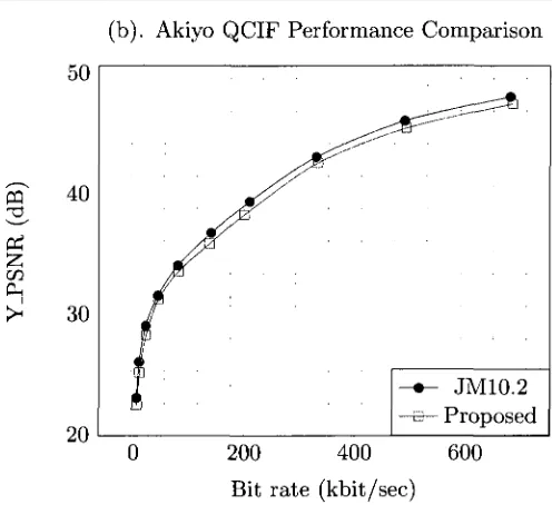
3.1 Intra4x4 prediction order 21 3.2 Intra4x4 prediction modes 22 3.3 Intra4x4 prediction process 23 3.4 Intra4x4 prediction architecture 24 3.5 Redundancy reduction algorithm 28 3.6 Comparison of SDS and SATD costs 30 3.7 News & Akiyo performance comparison 32

4.1 Relationship between bit rate and QP 35

4.2 Relationship of R C / Q P / R D O 37

4.3 Best initial QPs 41 4.4 Bit rates with different deviation 42

4.5 Intelligent grouping by deviation 44 4.6 QPs determination by deviation 46

4.7 Slice rate control 48 4.8 Comparisons of bitrate and performance of "Fancb" 50

4.9 Visual comparison of scene change 52

5.1 Storage system using MPEG-2 to H.264/AVC transcoding 54

5.2 MPEG-2 to H.264/AVC transcoding architecture 55

5.3 Field to frame motion vector mapping 59 5.4 Reference picture mapping of motion vector: P to P mapping 60

5.5 Reference picture mapping of motion vector: B to P mapping 61 5.6 Deriving motion vectors for inter_16x8 macroblock partitions with DWA 62

5.7 Deriving motion vectors for inter_8xl6 macroblock partitions with DWA 63 5.8 Deriving motion vectors for inter_8x8 macroblock partitions with DWA 64

5.9 EWA weighting masks 64 5.10 Error-variance weighted mapping for inter_8x8 block 65

5.11 Number of test modes vs. accuracy. 68

(11)

LIST OF FIGURES

5.15 Motion mapping with B performance 74

6.1 RVC framework 79 6.2 RVC VLD binary searching tree 82

6.3 RVC CAL model of MPEG-4 simple profile 84

6.4 RVC VLD function unit 84 6.5 XSLT transformation process: BSDL to CAL 86

7.1 DV data type 92 7.2 DV decoder data processing block diagram 92

7.3 DV-FU partition &z implementation 94

(12)

LIST OF TABLES

List of Tables

2.1 H.264/AVC profiles 13

3.1 Reducing intra4x4 prediction redundancy 25

3.2 Execution cycles for each MB 32

4.1 Performance & mismatch comparison 51

5.1 Performances comparison 75

6.1 VLC table of MPEG B-6 83 6.2 Generated VLC table of MPEG B-6 83

7.1 Formats of DV standards 91 7.2 FUs reusability of DV 96 7.3 Comparison between C code and RVC-CAL 97

B.l Definition of intra4x4 prediction modes 113

(13)

LIST OF TABLES

List of Abbreviations

3 G P P 3rd Generation Partnership Project

A A U X Audio Auxiliary Information

AS AAUX Source

A S C AAUX Source Control

ASO Arbitrary Slice Ordering

AVC Advanced Video Coding

B Bidirectional Frame

B G Binary Group

B P H.264/AVC Baseline Profile

B P P Bit Rate Per Picture

B S D L Bitstream Syntax Description Language

CAL Caltrop Actor Language

C A B A C Context-Adaptive Binary Arithmetic Coding

CAVLC Context-Adaptive Variable-Length Coding

C B R Constant Bit Rate

C B P Coded Block Pattern

D C T Digital Cosine Transfer

D D L Decoded Description Language

D I F Digital Interface

D V Digital Video

(14)

LIST OF TABLES

D W A Distance Weighted Average

EI Entropy Information

EWA Error-variance Weighted Average

F C B R Frame based Constant Bit Rate

F M O Flexible Macroblock Ordering

F S M Finite State Machine

F U Function Units

G O P Group of Picture

H . 2 6 4 / A V C Advanced Video Coding standard

H D High Definition

H D - T V High Definition TV

I D C T Inverse Digital Cosine Transfer

I Intra Frame

IM Intral6 DC Mode

IQ Inverse Quantization

IRSL Image and Remote Sensing Laboratory

I T U International Telecommunication Union

J V T Joint Video Team

LOC Lines Of Code

LoG Laplacian of Gaussian

M A D Mean Absolute Different

M B Macro Block

M B A F F MacroBlock Adaptive Frame/Field

M C Motion Compression

M E Motion Estimation

M P H.264/AVC Main Profile

M P E G ISO/IEC Moving Picture Experts Group

(15)

LIST OF TABLES

M R F Multiple Reference Frames

M S E Mean Square Error

M V Motion Vector

M V C Multiview Video Coding Standard

N A L Network Adaptation

N T S C National Television System Committee

P Predicted Frame

PAL Phase Alternating Line

P D A Personal Digital Assistant

P S N R Peak Signal to Noise Ratio

Q Quantization

QP Quatization Parameter

Q S M C Quarter Sub-pixel Mmotion Compensation

R-Q Rate-Quantization

R C Rate Control

R D O Rate-Distortion Optimized

RS Redundant Slices

RTL Register Transfer Level

RVC Reconfigurable Video Coding

S A D Sum of Absolute Different

SD Standard Definition

SI switching intra

SP switching predictive

SSD Sum of Squared Distortion

STAD Sum of Transformation Absolute Distortion

SVC Scalable Video Coding Standard, the scalable extension of H.264/AVC

T C Time Code

(16)

LIST OF TABLES

V A U X Video Auxiliary Information

V B R Variable Bit Rate

V B S Variable Block Size

V C E G Video Coding Experts Group

V C E G ITU-T Video Coding Expert Group

VCL Video Coding Layer

V L C Variable Length Coding

V L D Variable Length Decoding

X M L Extensible Markup Language

VS VAUX Source

V S C VAUX Source Control

X P H.264/AVC Extended Profile

XSL Extensible Stylesheet Language

XSLT Extensible Stylesheet Language Transformations

(17)

Chapter 1 Introduction

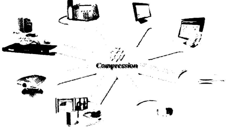
Digital multimedia systems, such as digital television and video streaming over the Internet,

belong to the everyday life of many people as shown in Fig. 1.1. Due to the fact that

uncom-pressed video requires a huge bandwidth, the input video is comuncom-pressed by the source coder

to a desired bit rate. The encoder performs lossy video signal compression. Then, the data

is transmitted to the receiver side via a transmission channel. The receiver performs inverse

operations to obtain a reconstructed video signal for display.

-r /- /

* f t / _{4 fSf}

/

&

^ / /

(18)

1.1. MOTIVATIONS & CONTRIBUTIONS

Continuous emergence of video coding standards on one side, and the growth in

develop-ment and impledevelop-mentation technology for them on the other side, have undoubtedly created a

whole new world of multimedia. So far, contributions to video coding technology have mainly

focused on improving coding efficiency. The challenges remain: not only to find efficient

cod-ing algorithms which require both simplification and high performance but also to reduce the

design time and avoid repeating design. This thesis starts with finding efficient algorithms for

the latest video coding standard, H.264/AVC, and then moves on a transition methodology

from the most prevalent video coding standard, MPEG-2, to the most efficient video coding

standard, H.264/AVC. Finally, a reconfigurable video coding framework is presented to reduce

development time.

1.1 Motivations & Contributions

Video coding standard is a large scope and it is impossible for a thesis work to overcome all

the issues. In this thesis, three major problems are emphasized: Low-complexity and efficient

H.264/AVC algorithms, MPEG-2/H.264 transcoding methodology and reconfigurable video

coding framework implementation.

At first, the latest video coding standard, H.264/AVC, is getting more attention due to its

high compression efficiency. However, higher computational complexity has to be paid for the

advantage. Being four times higher computational complexity than its counterpart, MPEG-2,

is considered an obstacle to implement it in real-time. Therefore, many research works focus on

how to reduce the computational complexity of H.264/AVC. The intra4x4 prediction is main

contribution of H.264/AVC. The available research results do not make full use of the features

of the intra4x4 prediction so that processing time is increased and is not suitable for real-time

process. The thesis proposes a new parallel processing structure to reduce the processing time

by carefully analysing the feature of H.264/AVC intra4x4 prediction [1], On the other hand,

rate control is playing a crucial role with limited bandwidth. How to improve video quality

in constant bit rate (CBR) is a great concern. In this thesis, a deviation based rate control

algorithm reasonably solves this problem for intra frame [2]. Two new encoder schemes are

also proposed in this thesis.

(19)

1.2. THESIS ORGANIZATION

is still used prevalently when the newer standard emerges. Apparently, to deal with this

problem, the transcoding algorithms are required. A universal transcoder, which can transcode

between any video formats, is not realistic. In this thesis, the methodology to transcode the

most prevalent video format, MPEG-2, to the latest video format, H.264/AVC, is presented

[3-5],

Finally, multiple codec standards need to be supported because more and more video

stan-dards are deployed. Although different, all coding stanstan-dards use the same or very similar

coding tools and hence share similar architectures and implementations. Unfortunately, the

way in which the existing coding standards are specified lacks flexibility to adapt performances

and complexity when new applications emerge. Therefore, repeating design and long

develop-ment time are imperative. A framework methodology using tools library has been proposed

by MPEG organization. The reconfigurable video coding (RVC) standard intends to create a

framework containing existing coding technology for developing, beside current standard

de-coders, new configurations for satisfying specific application constraints. However, some issues

still exist in that it is a brand new standard, such as, how to separate the variable length

de-coding (VLD) from the decoder parser unit? how to implement a new video de-coding standard

with RVC framework, and how to utilize the available function units (FUs) in design? the

author contributes an efficient data flow based implementation of the variable length decoding

(VLD) process particularly adapted for the instantiation and synthesis of CAL parses in the

MPEG RVC framework in the paper [6]. Three contributions [7-9] have been adopted by

MPEG RVC CAL reference code. The research work also models DV/DVCPRO video coding

standard with the MPEG RVC framework [10].

1.2 Thesis Organization

The research work presented in this thesis is categorized into four parts as shown in Fig. 1.2.

There are eight chapters included in this thesis. Chapter 1 introduces the motivation of this

thesis. The video coding standards are reviewed in Chapter 2, the focus being on those

features that are relevant for the thesis. The second part of this thesis presents how to reduce

the computational complexity and implement efficient rate control process for H.264/AVC.

(20)

1.2. THESIS ORGANIZATION

Thesis Structure

I f } 1

Introduction & H.264/AVC

Background Algorithms

Transcoding Reconfigurable video coding

I 1

Chapterl Chapter2 Chapter3 Chapter4 Thesis Video coding Intra 4x4 H.264/AVC introduction background prediction rate control

Chapter5 Chapter6 Chapter7 MPEG-2/H.264 MPEG-4 SP DV/DVCPRO

transcoding RVC RVC

Figure 1.2: Thesis structure.

process methodology. Chapter 4 deals with an efficient rate control algorithm of H.264/AVC. The rate control algorithm is the most important part in H.264/AVC standard, particularly in today, when the video is transmitted on net with limited bandwidth. The third part implements MPEG-2 to H.264/AVC transcoding. The main issues and methodologies of transcoding are presented in Chapter 5. The fourth part launches a new video coding standard, a framework video coding process, which is being developed by MPEG organization. In this part, Chapter 6 presents novel methodology to automatically generating variable length decoding table for RVC. Chapter 7 successfully implements DV/DVCPRO video coding standard with RVC-CAL. In the end, Chapter 8 provides a summary of this work. Some future research directions have been proposed in the same chapter.

(21)

Chapter 2 Background

In this chapter, some background knowledge about video compression is provided. A more

complete discussion on this subject can be found in books [11-15] and specifications [16-21],

such as, video compression methods, video coding standards, profile, level, motion vector,

macroblock, and peak signal-to-noise ratio (PSNR).

2.1 Video Coding Compression Principle

2 . 1 . 1 E x p l o i t i n g T e m p o r a l R e d u n d a n c i e s

Since a video is essentially a sequence of pictures sampled at a discrete frame rate, two

suc-cessive frames in a video sequence look largely similar. The extent of similarity between two

successive frames depends on how closely they are sampled (frame interval) and the motion of

the objects in the scene. Exploiting the temporal redundancies accounts for majority of the

compression gains in video encoding.

Since two successive frames are similar, taking the difference between the two frames results

in a smaller amount of data to be encoded. In general, the video coding technique that uses

the data from a previously coded frame to predict the current frame is called predictive coding

technique. The computation of the prediction is the key to efficient video compression. The

simplest form of predictive coding is frame difference coding, where, the previous frame is

(22)

2.1. VIDEO CODING COMPRESSION PRINCIPLE

sequence increases resulting in a loss of correlation between collocated pixels in two successive

frames.

Object motion is common in video and even a small motion of 1 to 2 pixels can lead to

loss of correlation between corresponding pixels in successive frames. Motion compensation

(MC) is used in video compression to reduce the correlation lost due to object motion [11].

The object motion in the real world is complex but for the purpose of video compression, a

simple translational motion is assumed.

2.1.1.1 Block B a s e d Motion Estimation

If we observe two successive frames of a video, the amount of changes within small NxN pixel

regions of an image are small. Assuming a translational motion, the NxN regions can be

better predicted from a previous frame by displacing the NxN region in the previous image

by an amount representing the object motion. The amount of this displacement depends on

relative motion between the two frames. For example, if there is a 5 pixel horizontal motion

between the frames, it is likely that a small NxN region will have a better prediction if the

prediction comes from a NxN block in the previous image displaced by 5 pixels. The process

of finding a predicted block that minimizes the difference between the original and predicted

blocks is called motion estimation (ME) and the resulting relative displacement is called a

motion vector [11]. When motion compensation is applied to the prediction, the motion vector

is also coded along with the pixel differences.

Video frames are typically coded one block at a time to take advantage of the motion

compensation applied to small NxN blocks. As the block size decreases, the amount of changes

within a block also typically decrease and the likelihood of finding a better prediction improves.

Similarly, as the block size increases, the prediction accuracy decreases. The downside to using

a smaller block size is that the total number of blocks in an image increases. Since each of the

blocks also has to include a motion vector to indicate the relative displacement, the amount

of motion vector information increases for smaller block sizes.

The best prediction for a given block can be found if the motion of the block relative to

a reference picture can be determined. Since translational motion is assumed, the estimated

(23)

process of forming a prediction thus requires estimating the relative motion of a given NxN

block. A simple approach to estimating the motion is to consider all possible displacements

in a reference picture and determine which of these displacements gives the best prediction.

The best prediction will be very similar to the original block and is usually determined using a

metric such the minimum sum of absolute differences (SAD) of pixels or the minimum sum of

squared differences (SSD) of pixels. The SAD has lower computational complexity compared

to the SSD computation and equally good in estimating the best prediction. The number

of possible displacements (motion vectors) of a given block is a function of the maximum

displacement allowed for motion estimation. Fast motion estimation (FME) [22] has been an

active area of research and a number of efficient algorithms have been developed.

2.1.1.2 Block B a s e d Motion Compensation

Motion compensation describes a picture in terms of the transformation of a reference picture

to the current picture. The reference picture may be previous in time or even from the future.

When images can be accurately synthesized from previously transmitted/stored images, the

compression efficiency can be improved. Motion compensation exploits the fact that, often,

for many frames of a movie, the only difference between one frame and another is the result of

either the camera moving or an object in the frame moving. In reference to a video file, this

means much of the information that represents one frame will be the same as the information

used in the next frame. Motion compensation takes advantage of this to provide a way to

create frames of a movie from a reference frame [12].

In block motion compensation (BMC), the frames are partitioned in blocks of pixels (e.g.

macroblocks of 16x16 pixels in MPEG). Each block is predicted from a block of equal size in

the reference frame. The blocks are not transformed in any way apart from being shifted to

the position of the predicted block. This shift is represented by a motion vector.

To exploit the redundancy between neighboring block vectors, (e.g. for a single moving

object covered by multiple blocks) it is common to encode only the difference between the

current and previous motion vector in the bit stream. The result of this differencing process

(24)

distribution of the motion vectors around the zero vector to reduce the output size.

2 . 1 . 2 E x p l o i t i n g S p a t i a l R e d u n d a n c i e s

In natural images, there exists a significant correlation between neighboring pixels. Small

areas within a picture are usually similar. Redundancies exist even after motion compensation.

Exploiting these redundancies will reduce the amount of information to be coded. Prediction

based on neighboring pixels, called intra prediction [11], is also used to reduce the spatial

redundancies. Transform techniques are used to reduce the spatial redundancies substantially.

The spatial redundancy exploiting transforms such as the discrete cosine transform (DCT),

transform a NxN picture block into NxN block of coefficients in another domain called the

frequency domain [23], The key properties of these transforms that make them suitable for

video compression are energy compaction and de-correlation. When the transform is applied,

the energy of a NxN pixel block is compacted into a few transformed coefficients and the

correlation between the transformed coefficients is also reduced substantially. This implies

that significant amount of information can be recovered by using just a few coefficients. The

transform coefficients in the frequency domain can be roughly classified into low, medium,

and high spatial frequencies [13]. Since the human visual system is not sensitive to the high

spatial frequencies, the transform coefficients corresponding to the high frequencies can be

discarded without affecting the perceptual quality of the reconstructed image. As the number of

discarded coefficients increases, the compression increases, and the video quality decreases. The

coefficient dropping is in fact exploiting the perceptual redundancies. Another way of reducing

the perceptual redundancies is by quantizing the transform coefficients. The quantization

process reduces the number of levels [21] while still retaining the video quality. As with

coefficient dropping, as the quantization step size increases, the compression increases, and the

video quality decreases.

2 . 1 . 3 E x p l o i t i n g S t a t i s t i c a l R e d u n d a n c i e s

The transform coefficients, motion vectors, and other data have to be encoded using binary

codes in the last stage of video compression. The simplest way to code these values is by using

(25)

2.2. IMAGE/VIDEO CODING ROADMAP

and using fixed length codes is wasteful. Average code length can be reduced by assigning

shorter code words to values with higher probability. Variable length coding is used to exploit

these statistical redundancies and increase compression efficiency further.

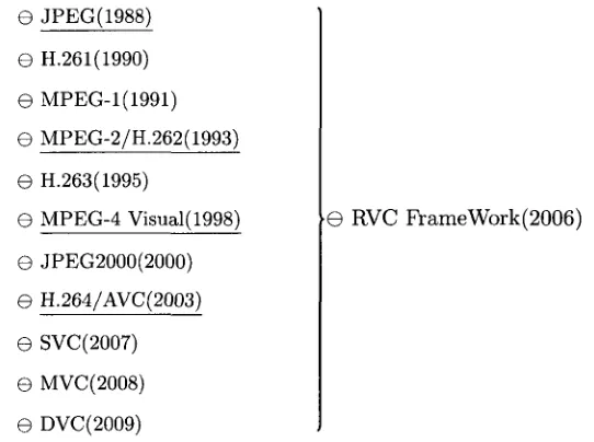
2.2 Image/Video Coding Roadmap

The multimedia compression standards have been developing for decades as shown in Fig.2.1.

The Moorse's law [24] of compression shows that the performance has been doubled every five

years, which means the standard is able to obtain roughly 50% gain in about five years. In the

mean time, the computational complexity also increases dramatically.

G H.261(1990)

RVC FrameWork(2006)

Figure 2.1: Image/Video coding standards development roadmap.

2.3 Video Coding Standards Overview

2 . 3 . 1 H . 2 6 1 / H . 2 6 3

The H.261 [17] and H.263 [19] are not international standards but only recommendations of

the ITU. They are both based on the same technique as the MPEG standards and can be seen

as simplified versions of MPEG video compression. They were originally designed for video

(26)

2.3. VIDEO CODING STANDARDS OVERVIEW

use. The conclusion is therefore that H.261 and H.263 are not suitable for usage in general

digital video coding.

2 . 3 . 2 M P E G - 1

The first public standard of the MPEG committee was the MPEG-1, ISO/IEC 11172 [16],

whose first parts were released in 1993. MPEG-1 video compression is based upon the same

technique that is used in JPEG. In addition to that, it also includes techniques for efficient

coding of a video sequence. In Motion JPEG/Motion JPEG 2000, each picture in the sequence

is coded as a separate unique picture resulting in the same sequence as the original one. In

MPEG video, only the new parts of the video sequence is included together with information

of the moving parts. MPEG-1 is focused on bit streams of about 1.5 Mbps and originally

for storage of digital video on CDs. The focus is on compression ratio rather than picture

quality. It can be considered as traditional VCR quality but digital instead. It is important to

note that the MPEG-1 standard, as well as MPEG-2, MPEG-4 and H.264 that are described

below, defines the syntax of an encoded video stream together with the method of decoding

this bit stream. Thus, only the decoder is actually standardized. A MPEG encoder can be

implemented in different way and a vendor may choose to implement only a subset of the

syntax, providing it provides a bit stream that is compliant with the standard. This allows

for optimization of the technology and for reducing complexity in implementations. However,

it also means that there are no guarantees for quality - different vendors implement MPEG

encoders that produce video streams that differ in quality.

2 . 3 . 3 M P E G - 2

The MPEG-2 project focused on extending the compression technique of MPEG-1 to cover

larger pictures and higher quality at the expense of a higher bandwidth usage. MPEG-2,

ISO/IEC 13818 [18], also provides more advanced techniques to enhance the video quality at

the same bit rate. The expense is the need for far more complex equipment. As a note, DVD

(27)

2 . 3 . 4 M P E G - 3

The next version of the MPEG standard, MPEG-3 was designed to handle HDTV, however,

it was discovered that the MPEG-2 standard could be slightly modified and then achieve the

same results as the planned MPEG-3 standard. Consequently, the work on MPEG-3 was

discontinued.

2 . 3 . 5 M P E G - 4

The next generation of MPEG, MPEG-4, is based upon the same technique as MPEG-1 and

MPEG-2. Once again, the new standard focused on new applications. The most important new

features of MPEG-4, ISO/IEC 14496 [20] and concerning video compression are the support

of even lower bandwidth consuming applications, e.g. mobile devices like cell phones, and on

the other hand applications with extremely high quality and almost unlimited bandwidth. In

general the MPEG-4 standard is wider than the previous standards. It also allows for any frame

rate, while MPEG-2 was locked to 25 frames per second in PAL and 30 frames per second in

national television system committee (NTSC). When "MPEG-4" is mentioned in surveillance

applications today it is usually 4 part 2 that is referred to. This is the "classic"

MPEG-4 video streaming standard, a.k.a. MPEG-MPEG-4 Visual. Some network video streaming systems

specify support for "MPEG-4 short header", which is a H.263 video stream encapsulated with

MPEG-4 video stream headers. MPEG-4 short header does not take advantage of any of the

additional tools specified in the MPEG-4 standard, which gives a lower quality level than both

MPEG-2 and MPEG-4 at a given bit rate.

2 . 3 . 6 H . 2 6 4 / A V C

H.264/AVC is the latest generation standard for video encoding. This initiative has many goals.

It should provide good video quality at substantially lower bit rates than previous standards

and with better error robustness - or better video quality at an unchanged bit rate. The

standard is further designed to give lower latency as well as better quality for higher latency.

(28)

allow the standard to be applied to a wide variety of applications: for both low and high bit

rates, for low and high resolution video, and with high and low demands on latency. The

following three profiles were defined in the original standard, and remain unchanged in the

latest version:

• Baseline Profile (BP): Primarily for low-cost applications that require additional data

loss robustness, this profile is used in some videoconferencing and mobile applications.

This profile includes all features that are supported in the Constrained Baseline Profile,

plus three additional features that can be used for loss robustness (or for other purposes

such as low-delay multi-point video stream composition).

• Extended Profile (XP): This profile is used for standard-definition digital TV broadcasts

that use the MPEG-4 format as defined in the DVB standard [25]. It is not, however,

used for high-definition television broadcasts, as the importance of this profile faded when

the High Profile was developed in 2004 for that application.

• Main Profile (MP): Intended as the streaming video profile, this profile has relatively

high compression capability and some extra tricks for robustness to data losses and

server stream switching.

Table 2.1 gives a high-level summary of the coding tools included in these profiles. The

baseline profile includes intra (I) and predictive (P)-slices, some enhanced error resilience tools

(flexible macroblock ordering (FMO), arbitrary slice ordering (ASO), and redundant slices

(RS)), and context adaptive variable length coding (CAVLC). It does not contain bidirectional

(B), switching predictive (SP), and switching intra (SI) slices, interlace coding tools or

context-adaptive binary arithmetic coding (CABAC) entropy coding. The extended profile is a

super-set of baseline, adding B, SP and Si-slices and interlace coding tools to the super-set of baseline

profile coding tools and adding further error resilience support in the form of data partitioning

(DP). It does not include CABAC. The main profile includes I, P and B-slices, interlace coding

tools, CAVLC and CABAC. It does not include enhanced error resilience tools (FMO, ASO,

(29)

Table 2.1: H.264/AVC profiles.

Coding Tools Baseline Main E x t e n d e d

I and P Slices / / /

CAVLC / / /

CABAC /

B Slices / /

Interlaced Coding (PicAFF, MBAFF) / /

Enhanced Error Resil. (FMO, ASO, RS) / /

Further Enh. Error Resil (DP) /

SP and SI Slices /

2 . 3 . 7 M P E G - 7

MPEG-7 [26] is a different kind of standard as it is a multimedia content description standard,

and does not deal with the actual encoding of moving pictures and audio. With

MPEG-7, the content of the video (or any other multimedia) is described and associated with the

content itself, for example to allow fast and efficient searching in the material. MPEG-7 uses

extensible markup language (XML) to store metadata, and it can be attached to a timecode

in order to tag particular events in a stream. Although MPEG-7 is independent of the actual

encoding technique of the multimedia, the representation that is defined within MPEG-4, i.e.

the representation of audio visual data in terms of objects, is very well suited to the MPEG-7

standard. MPEG-7 is relevant for video surveillance since it could be used for example to tag

the contents and events of video streams for more intelligent processing in video management

software or video analytics applications.

2 . 3 . 8 M P E G - 2 1

MPEG-21 [27] is a standard that defines means of sharing digital rights, permissions, and

restrictions for digital content. It aims at defining an open framework for multimedia

ap-plications. MPEG-21 is ratified in the standards ISO/IEC 21000 - Multimedia framework

(MPEG-21). MPEG-21 is a XML-based standard, and is developed to counter illegitimate

distribution of digital content.

MPEG-21 is based on two essential concepts: the definition of a fundamental unit of

(30)

2.4. FRAME TYPES

with them. Digital items can be considered the kernel of the multimedia framework and the

users can be considered as who interacts with them inside the multimedia framework. At its

most basic level, MPEG-21 provides a framework in which one user interacts with another one,

and the object of that interaction is a digital item. Due to that, we could say that the main

objective of the MPEG-21 is to define the technology needed to support users to exchange,

access, consume, trade or manipulate digital items in an efficient and transparent way.

2.4 Frame Types

The basic principle for video compression is the image-to-image prediction. The first image

is called an I-frame and is self-contained, having no dependency outside of that image. The

following frames may use part of the first image as a reference. An image that is predicted

from one reference image is called a P-frame and an image that is bidirectionally predicted

from two reference images is called a B-frame.

1. I-frames: Intra predicted, self-contained;

2. P-frames: Predicted from last I or P reference frame;

3. B-frames: Bidirectional; predicted from two references one in the past and one in the

future, and thus out of order decoding is needed;

Figure 2.2 shows how a typical sequence with I-, B-, and P-frames may look. Note that

a P-frame may only reference a preceding I- or P-frame, while a B-frame may reference both

preceding and succeeding I- and P-frames. The video decoder restores the video by decoding

the bit stream frame by frame. Decoding must always start with an I-frame, which can be

decoded independently, while P- and B-frames must be decoded together with current reference

image(s).

2.5 Group of Pictures

One parameter that can be adjusted in MPEG-4 is the Group of Pictures (GOP) length and

structure, also referred to as Group of Video (GOV) in some MPEG standards. It is normally

repeated in a fixed pattern, for example:

(31)

2.6. VARIABLE AND CONSTANT BIT RATE

Figure 2.2: Picture types.

1. GOV = 4, e.g. I P P P I P P P ... ;

2. GOV = 15, e.g. I P P P P P P P P P P P P P P I P P P P P P P P P P P P P P ... ;

3. GOV = 8, e.g. IBPBPBPB IBPBPBPB ... ;

The appropriate GOP depends on the application. By decreasing the frequency of I-frames,

the bit rate can be reduced. By removing the B-frames, latency can be reduced. The number

of frames between two I-frames, can be adjusted to fit the application.

2.6 Variable and Constant Bit Rate

Another important aspect of MPEG is the bit rate mode that is used. In most MPEG

sys-tems, it is possible to select the mode, constant bit rate (CBR) or variable bit rate (VBR).

The optimal selection depends on the application and available network infrastructure. With

limited bandwidth available, the preferred mode is normally CBR as this mode generates a

constant and predefined bit rate. The disadvantage with CBR is that image quality will vary.

While the quality will remain relatively high when there is no motion in a scene, it will

signif-icantly decrease with increased motion. With VBR,, a predefined level of image quality can be

maintained regardless of motion or the lack of it in a scene. This is often desirable in video

surveillance applications where there is a need for high quality, particularly if there is motion

in a scene. Since the bit rate in VBR may vary even when an average target bit rate is defined

(32)

2.7. MPEG STANDARDS COMPARISON

capacity.

2.7 MPEG Standards Comparison

Looking at MPEG-2 and later standards, it is important to bear in mind that they are not

backwards compatible, i.e. strict MPEG-2 decoders/encoders will not work with MPEG-1.

Neither will H.264 encoders/decoders work with MPEG-2 or previous versions of MPEG-4,

unless specifically designed to handle multiple formats. However, there are various solutions

available where streams encoded with newer standards can sometimes be packetized inside

older standardization formats to work with older distribution systems. Since both

MPEG-2 and MPEG-4 cover a wide range of picture sizes, picture rates and bandwidth usage, the

MPEG-2 introduces a concept called Profile@Level [21]. This is created to make it possible to

communicate compatibilities among applications. For example, the studio profile of MPEG-4

is not suitable for a PDA and vice versa. Note that: MPEG-2, MPEG-4 and H.264/AVC are

all subject to licensing fees.

Since the H.261/H.263 recommendations are neither international standards nor offer any

compression enhancements compared to MPEG standards, they are not of any real interest and

are not recommended as suitable techniques for video surveillance. MPEG-1 is considered, in

most cases, more effective than Motion JPEG. However, for just a slightly higher cost, MPEG-2

provides even more advantages and supports better image quality, comprising of frame rate and

resolution. On the other hand, MPEG-2 requires more network bandwidth consumption and

is a technique of greater complexity. MPEG-4 is developed to offer a compression technique

for applications demanding less image quality and bandwidth. It is also able to deliver video

compression similar to MPEG-1 and MPEG-2, i.e. higher image quality at higher bandwidth

consumption.

If the available network bandwidth is limited, or if video is to be recorded at a high frame

rate and there are storage space restraints, MPEG may be the preferred option rather than

motion JPEG. It provides a relatively high image quality at a lower bit rate (bandwidth

usage). Still, the lower bandwidth demands come at the cost of higher complexity in encoding

and decoding, which in turn contributes to a higher latency when compared to motion JPEG.

(33)

2.8. PERFORMANCE METRIC

of motion pictures in many application areas, including video surveillance. As mentioned

above, it has already been implemented in as diverse areas as high-definition DVD (HD-DVD

and Blu-ray), for digital video broadcasting including high-definition TV (HDTV), in the 3rd

generation partnership project (3GPP) standard for the third generation mobile telephony and

in software such as QuickTime and Apple Computer's MacOS X operating system.

H.264 is now a widely adopted standard, and represents the first time that the ITU, ISO

and IEC have come together on a common, international standard for video compression [21],

H.264 entails significant improvements in coding efficiency, latency, complexity and robustness.

It provides new possibilities for creating better video encoders and decoders that provide higher

quality video streams at maintained bit rate (compared to previous standards), or, conversely,

the same quality video at a lower bit rate.

There will always be a market need for better image quality, higher frame rates, and higher

resolutions with minimized bandwidth consumption. H.264 offers this, and as the H.264 format

becomes more broadly available in network cameras, video encoders and video management

software, system designers and integrators will need to make sure that the products and vendors

they choose support this new open standard. And for the time being, network video products

that support several compression formats are ideal for maximum flexibility and integration

possibilities.

2.8 Performance Metric

Distortion measures the difference between the decoded image and the original image. Peak

signal to noise ratio (PSNR) is normally used to evaluated the distortion. PSNR is defined by

the following formula.

m—1n— 1

i=0 j=0

PSNR = 20 x logw( 255

(34)

2.9. CONCLUSIONS

Where, EMSE is the mean square error between an original m x n image I and its decoded

image I.

2.9 Conclusions

In this chapter, the video coding fundamentals have been presented. It starts with video coding

standards. Some basic terminologies and performance metric are also defined in this chapter.

These concepts help to understand the following chapters.

(35)

Chapter 3 Fast Implementation of H.264 4x4

Intra Prediction

3.1 Introduction

The Joint Video Team (JVT) of ISO/IEC MPEG and ITU-VCEG jointly developed a new video

compression standard H.264/AVC [21]. Compared to previous standards, such as MPEG-2,

H.263 and MPEG-4, aggressive compression techniques are employed in H.264/AVC standard.

As a result, its performance is greatly improved in terms of the compression efficiency, however,

this is achieved at the expense of increasing the computational complexity.

Intra prediction utilizes the spatial correlation in an image to predict the block being

en-coded from its nearby pixels. It is recognized to be one of the main factors contributing the

success of H.264/AVC [21]. To select the best prediction mode, the encoder has to search

all possible prediction modes exhaustively in order to encode blocks. As a result, the

com-putational complexity in H.264/AVC is extremely high. Some previous approaches to reduce

computation complexity of H.264/AVC intra prediction by optimizing and speeding up are

presented in [28-36].

In this chapter, a novel parallel architecture to achieve fast intra prediction is presented.

The remaining sections are organized as follows: In Section 3.2, the H.264/AVC intra prediction

is briefly introduced. Section 3.3 presents the proposed architecture, a redundancy reduction

(36)

3.2. H.264/AVC INTRA PREDICTION

of intra frame prediction. Section 3.4 provides simulation results and conclusions are addressed

in Section 3.5.

3.2 H.264/AVC Intra Prediction

In H.264/AVC baseline intra coding, two intra prediction modes for luminance component

are supported in each profile [21]. One is intra4x4 mode and the other is intral6xl6 mode.

The intra8x8 is a new prediction type defined in H.264/AVC FRExt [37]. For intra4x4 mode,

each MB is divided into sixteen non-overlapping 4x4 blocks. Each block can select one of

nine prediction modes. For intral6xl6 mode, four prediction modes are available for each

MB. Chroma intra prediction is independent to luminance prediction mode. Two chroma

components are simultaneously predicted with the same mode. The intra4x4 is more accurate

than intral6xl6, however it requires more bits to be coded. Hence, intra4x4 is used for highly

textured regions while intral6xl6 is used for plain regions.

From the complexity perspective, H.264/AVC encodes macroblocks (MBs) by iterating all

the luminance intra decisions for each possible chroma intra prediction mode to achieve the

best coding efficiency. Therefore, the number of mode combination for luminance and chroma

components in a MB is C8 x (L4 x 16 + L16), where C8, L4, and L16 represent the number

of modes for chroma prediction, 4x4 luminance prediction, and 16x16 luminance prediction

respectively. This means that, 4 x (9 x 16 + 4) = 592 different rate distortion optimization

(RDO) costs have to be calculated before a best mode can be determined. If the 8x8 luminance

prediction in H.264/AVC FRExt is included, the number of mode combination is C8 x (L4

x 16 + L8 x 4 + L16) = 4 x ( 9 x l 6 + 9 x 4 + 4) = 736. Even in low complexity

mode [38], 9 x 1 6 + 4 + 4 x 2 = 156 mode decisions are needed. Although low complexity

mode can greatly reduce computational load, encoding time still needs to be reduced for some

applications requiring very low delay. If the target application is high definition TV (HDTV),

each frame needs (1920 x 1080 x 592) / 256 = 4,795,200 calculations, which is not feasible for

real-time implementation. Thus, speeding up intra coding process is essentially required.

In H.264/AVC [21], intra prediction is performed in two modes, intra4x4 and intral6xl6

mode. The luminance samples in a MB is divided into sixteen 4x4 blocks. Then these blocks

(37)

3.2. H.264/AVC INTRA PREDICTION

0 4

y 7 5

/

<

1 2 y

- f

1 0 /

/

1 4 /

/

- k 5

Figure 3.1: Intra4x4 prediction order.

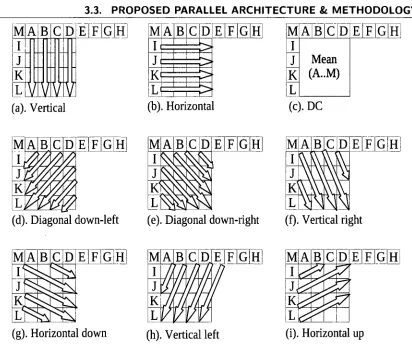
There are nine prediction modes for each 4x4 block in intra4x4 prediction mode as shown in

Fig. 3.2. They are one DC mode (mode2) and eight directional modes, e.g. vertical (modeO),

horizontal (model), diagonal down left (mode3), diagonal down right (mode4), vertical right

(mode5), horizontal down (mode6), vertical left (mode7) and horizontal up (mode8). To reflect

the edge trend of the block, the prediction for the current 4x4 block is calculated using the

boundary pixels of the previously decoded blocks above and to the left of it. Since the pixels

along the direction of the local edge have similar values, an accurate prediction can be achieved

if the direction of the prediction mode is the same as the edge direction of the block. In this

figure, neighboring samples used for prediction are labeled with capital letters A M. The 16

grey grids are the predicted samples called predictors. Each predictor is extrapolated from the

neighboring pixels A M. The extrapolation process is specified by H.264/AVC [21]. Definitions

of extrapolation equations for nine prediction modes are listed in Table B.l. Because each 4x4

block use neighboring samples to form predictors, the encoder needs to reconstruct the current

block before moves to the next block. Therefore, in the intra4x4 prediction, the block in the

upper left corner is processed at first and the lower right corner is processed at last. The intra

prediction for each block uses the pixels in its left and top sides as reference pixels. A block

thus can not be predicted until its previous block has been reconstructed. The reconstruction

includes discrete cosine transform (DCT), quantization (Q), inverse quantization (IQ), and

(38)

3.3. PROPOSED PARALLEL ARCHITECTURE &. METHODOLOGY

M A B

K

WN

E F G H

(a). Vertical

M A B C i D E F G H

t | —

KH

i r '

(b). Horizontal

M A B C D E F G H I

J K L

Mean (A..M)

(c). DC

(g). Horizontal down (h). Vertical left

(d). Diagonal down-left (e). Diagonal down-right (f). Vertical right

M A B C D E|F|G[H] I

J<

K, L r ^ L

(i). Horizontal up

Figure 3.2: Intra4x4 prediction modes.

3.3 Proposed Parallel Architecture & Methodology

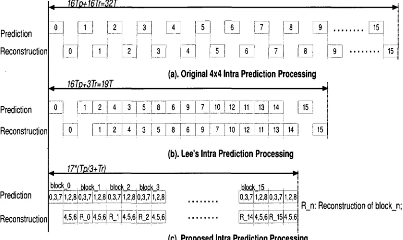
The original process handles blocks in serial, which is not efficient as illustrated in Fig. 3.3

(a). Efficient architectures have been reported in [28-31], however, they all have drawbacks

either with the pipelining architecture or in compression gains. Huang's work [28] has bubbles

between Intra4x4 predictions because of the low throughput of reconstruction process so that

the prediction has to wait for the completion of reconstruction. Lee's work [29] perfectly

pipelines the intra prediction and reconstruction process shown as Fig. 3.3 (b), however, it

requires that both intra prediction and reconstruction have exact equal processing cycles.

It also reduces some prediction modes in some blocks in order to enforce pipelining, hence,

the video quality is degraded. Jin's work [30] proposes both partially and fully pipelined

architectures for intra4x4 prediction and has the same drawback as the approach in [29].

Moreover, the architectures add dependency graph process in order to improve gains, however,

(39)

this increases hardware overhead. It takes 25 cycles to process each block, which is too long

for high throughput reconstruction. Suh's work [31] is similar to Huang's work, which takes

34 cycles to process each block. The thesis proposes an efficient parallel architecture followed

by a redundancy reduction algorithm to speed up the intra4x4 prediction.

Prediction

Reconstruction

Prediction

Reconstruction

16Tp+16Tr=32T

3 | | _ 4

tn

7J

16To+3Tr=19T

(a). Original 4x4 Intra Prediction Processing

Prediction 0 1 2 4 3 5 8 6 9 7 10 12 11 13 14 15

Reconstruction 0 1 2 4 3 5 8 6 9 7 10 12 11 13 14 15

(b). Lee's Intra Prediction Processing

17*(Tp/3+Tr)

block.0 block 1 _ block 2 block 3 0,3,7 1,2,8 0,3,7 1,2,8 0,3,7 1,2,8 0,3,7] 1,2,8

4,5,6 R 0 4,5,6 R_1 4,5,6 R_2 4,5,6

block 15 0,3,7 1,2,8 0,3,7 1,2,8

R_14 4,5,6 R_15 4,5,6

R_n: Reconstruction of block_n;

(c). Proposed Intra Prediction Processing

Figure 3.3: Intra4x4 prediction process.

3 . 3 . 1 P a r a l l e l A r c h i t e c t u r e

Although a data dependency truly exists among blocks in intra4x4 prediction, we can state,

after careful observation, that such data dependency does not exist in some intra4x4 prediction

modes. Therefore, they are able to be processed without waiting for their previous blocks to

be reconstructed, i.e., modeO, 3, and 7 of the current block can be simultaneously predicted

when its previous block is being reconstructed. After the reconstruction of its previous block

is complete, the rest of modes, i.e., model, 2, 8 and mode4, 5, 6 of the current block, shown

as Fig. 3.3 (c) can be predicted in parallel. The same procedure follows in the rest of the

blocks. To sum up, we divide nine prediction modes into three groups, and each group has

(40)

3.3. PROPOSED PARALLEL ARCHITECTURE & METHODOLOGY

The proposed architecture has four advantages compared to previous works. The first

advantage is that the proposed process does not ignore any prediction modes. The second

advantage is that the encoder follows that order specified in H.264/AVC standard to guarantee

the consistency between the encoder and the decoder. The third advantage is that it does not

require the processing cycles of intra prediction and reconstruction to be exact the same. The

last advantage is that the proposed architecture can reduce total processing time of each MB

to 17 x (1/3TP + Tr) if high throughput reconstruction is adopted, where Tp is prediction time

and Tr is reconstruction time.

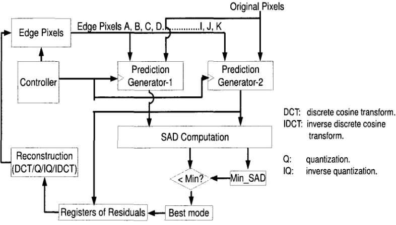
As shown in Fig. 3.4, the Iuma4x4 prediction unit mainly consists of five functional blocks

for Prediction Generator-1, Prediction Generator-2, SAD (sum of absolute difference)

Com-putation, Reconstruction, and Controller. Prediction Generator-1 and Prediction Generator-2

calculate the predicted pixel values for all the intra modes. SAD Computation block calculates

SAD values for each mode in order to make mode decision. Reconstruction block recovers the

prediction pixels of the best mode by the reconstruction process (DCT, Q, IQ, and IDCT). The

Controller block selects the right pixels from Edge Pixels buffer and feeds them into Prediction

Generator blocks.

Figure 3.4: Intra4x4 prediction architecture.

(41)

In the first step, the Generator-1 is parallel with the reconstruction process and the first

group (modeO, 3 and 7) are predicted in this step. In the second step, the Generator-1 and

Generator-2 are parallel to process the second group (model, 2, and 8) and the third group

(mode4, 5 and 6). The output of Edge Pixels unit are selected by the controller. Each group

has its own best mode by calculating SAD. The final best mode is obtained by comparing the

best mode of each group. Meanwhile, the residuals of this block with the best mode are written

into the register. The reconstruction process implements DCT, Q, IQ and IDCT based on the

residuals. After added to the values of prediction, the reconstructed edges pixels are stored in

the buffer for being used for predicting the next block.

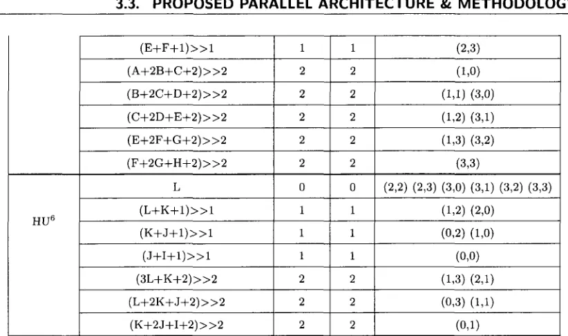
3 . 3 . 2 R e d u n d a n c y R e d u c t i o n A l g o r i t h m

Considering the definition of the nine intra4x4 prediction modes of H.264/AVC [21] as shown

in Appendix Table B.l, there are some identical parts in calculating the predicted values. It is

possible to reduce memory access and improve prediction time by eliminating these redundancy

computations. A detailed summary is listed in Table 3.1. In this table, identical prediction

items exist not only in different pixels of the same mode, but also in different pixels of different

modes, for example, the predicted value of both pixels (1, 0) and (0, 1) in diagonal down left

prediction mode is equal to the value in pixel (3, 0) of diagonal down right prediction mode.

Therefore, the redundancy computations are able to be reduced.

Table 3.1: Reducing intra4x4 prediction redundancy.

M o d e Equation R o u n d Shift Positions (x, y )

A 0 0 (0,0) (1,0) (2,0) (3,0) Vertical

B 0 0 (0,1) (1,1) (2,1) (3,1) Vertical

C 0 0 (0,2) (1,2) (2,2) (3,2) D 0 0 (0,3) (1,3) (2,3) (3,3) I 0 0 (0,0) (0,1) (0,2) (0,3) Horizontal

J 0 0 (1,0) (1,1) (1,2) (1,3) Horizontal

K 0 0 (2,0) (2,1) (2,2) (2,3) L 0 0 (3,0) (3,1) (3,2) (3,3) DC ( I + J + K + L + A + B + C + D + 4 ) » 3 4 3 ALL

( A + 2 B + C + 2 ) » 2 2 2 (0.0) n m 1

(42)

( C + 2 D + E + 2 ) » 2 2 2 (0,2) (1,1) (2,0) ( D + 2 E + F + 2 ) » 2 2 2 (0,3) (1,2) (2,1) (3,0) ( E + 2 F + G + 2 ) » 2 2 2 (1,3) (2,2) (3,1) ( F - ( - 2 G + H + 2 ) » 2 2 2 (2,3) (3,2)

( G + 3 H + 2 ) » 2 2 2 (3,3) ( L + 2 K + J + 2 ) » 2 2 2 (3,0) DDR2

( K + 2 J + I + 2 ) » 2 2 2 (2,0) (3,1) DDR2

( J + 2 I + M + 2 ) > > 2 2 2 (1,0) (2,1) (3,2) ( I + 2 M + A + 2 ) » 2 2 2 (0,0) (1,1) (2,2) (3,3) ( M + 2 A + B + 2 ) » 2 2 2 (0,1) (1,2) (2,3) ( A + 2 B + C + 2 ) » 2 2 2 (1.3) ( B + 2 C + D + 2 ) » 2 2 2 (0,3)

( M + A + l ) » l 1 1 (0,0) (2,1) VR3

( A + B + l ) » l 1 1 (0,1) (2,2) VR3

( B + C + l ) » l 1 1 (0,2) (2,3) ( C + D + l ) » l 1 1 (0,3) ( K + 2 J + I + 2 ) » 2 2 2 (3,0) ( J + 2 I + M + 2 ) » 2 2 2 (2,0) ( I + 2 M + A + 2 ) » 2 2 2 (1,0) (3,1) ( M + 2 A + B + 2 ) » 2 2 2 _{(1.1) (3,2)} ( A + 2 B + C + 2 ) » 2 2 2 (1,2) (3,3) ( B + 2 C + D + 2 ) » 2 2 2 (1.3)

( L + K + l ) » l 1 1 (3,0) HD4

( K + J + l ) » l 1 1 (2,0) (3,2) HD4

( J + I + l ) » l 1 1 (1,0) (2,2) ( I + M + l ) » l 1 1 (0,0) (1,2) ( L + 2 K + J + 2 ) » 2 2 2 (3,1)

( K + 2 J + I + 2 ) » 2 2 2 (2,1) (3,3) ( J + 2 I + M + 2 ) » 2 2 2 _{(1.1) (2,3)} ( I + 2 M + A + 2 ) » 2 2 2 (0,1) (1,3) ( M + 2 A + B + 2 ) » 2 2 2 (0,2) ( A + 2 B + C + 2 ) » 2 2 2 (0,3) ( A + B + l ) » l 1 1 (0,0) VL5

( B + C + l ) » l 1 1 (0,1) (2,0) VL5

( C + D + l ) » l 1 1 (0,2) (2,1) ( D + E + l ) » l 1 1 (0,3) (2,2)

(43)

( E + F + l ) » l 1 1 (2,3) ( A + 2 B + C + 2 ) > > 2 2 2 _(1,0) ( B + 2 C + D + 2 ) » 2 2 2 (1,1) (3,0) ( C + 2 D + E + 2 ) > > 2 2 2 _(1.2)_(3,1) ( E + 2 F + G + 2 ) » 2 2 2 (1,3) (3,2) ( F + 2 G + H + 2 ) » 2 2 2 (3,3)

L 0 0 (2,2) (2,3) (3,0) (3,1) (3,2) (3,3) HU6

( L + K + l ) » l 1 1 (1,2) (2,0) HU6

( K + J + l ) » l 1 1 (0,2) (1,0) ( J + I + l ) » l 1 1 (0,0) ( 3 L + K + 2 ) » 2 2 2 (1.3) (2,1)

( L + 2 K + J + 2 ) » 2 2 2 (0,3) (1,1) ( K + 2 J + I + 2 ) » 2 2 2 (0,1)

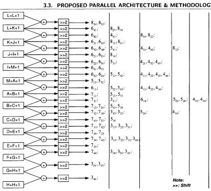
Figure 3.5 illustrates how to calculate 6 prediction modes (except DC, vertical and

hor-izontal prediction modes) with the common parts. The 14 common parts are listed on the

left side of Fig. 3.5. The terms ("A" to "M") of the common parts indicate the neighbouring

pixels as shown in Fig. 3.2. The numbers Nxy on the right side in Fig. 3.5 refer to mode N

in position (x, y ). For example, the predicted value in pixel (1, 1) of diagonal down left mode,

( A + 2 B + C + 2 ) > > 2 , can be calculated by adding "(A+B)" and "(B+C)". By analysis, only

14 common parts and 23 equations of their combination are required for intra4x4 prediction

calculations, which can be implemented by 27 adders and 23 shifts. Moreover, the DC

pre-diction mode is very straightforward, which only requires 3 adders and 1 shift. For vertical,

horizontal and part of horizontal up prediction modes, the predicted values can be obtained

only by propagating the values of edge pixels. Therefore, for total intra4x4 mode prediction,

the proposed algorithm requires 30 adders and 24 shifts. It can be completed within one cycle.

To achieve fast intra4x4 prediction, a high throughput reconstruction process is also

re-quired. The reconstruction process (DCT, Q, IQ, and IDCT) is implemented in parallel with

Algorithms & implementation of advanced video coding standards

Scholarship at UWindsor

Scholarship at UWindsor

Algorithms & implementation of advanced video coding

Algorithms & implementation of advanced video coding

standards

standards

Algorithms & Implementation

of Advanced Video Coding Standards

Jianjun Li

1 * 1

Abstract

Acknowledgements

Contents

List of Figures

List of Tables

List of Abbreviations

Chapter 1

Introduction

/

&

^ / /

I f } 1

I 1

Chapter 2

Background

Chapter 3

Fast Implementation of H.264 4x4

Intra Prediction

/

/

<

/

/

WN

tn

7J