University of Windsor University of Windsor
Scholarship at UWindsor
Scholarship at UWindsor
Electronic Theses and Dissertations Theses, Dissertations, and Major Papers
2019
Improving Document Representation Using Retrofitting
Improving Document Representation Using Retrofitting
Zeeshan Mansoor
University of Windsor
Follow this and additional works at: https://scholar.uwindsor.ca/etd
Recommended Citation Recommended Citation
Mansoor, Zeeshan, "Improving Document Representation Using Retrofitting" (2019). Electronic Theses and Dissertations. 7721.
https://scholar.uwindsor.ca/etd/7721
Improving Document Representation
Using Retrofitting
By
Zeeshan Mansoor
A Thesis
Submitted to the Faculty of Graduate Studies through the School of Computer Science in Partial Fulfillment of the Requirements for
the Degree of Master of Science at the University of Windsor
Windsor, Ontario, Canada
2019
c
Improving Document Representation Using Retrofitting
by
Zeeshan Mansoor
APPROVED BY:
G. Zhang
Department of Mechanical, Automotive and Materials Engineering
Z. Kobti
School of Computer Science
J. Lu, Advisor School of Computer Science
I hereby certify that I am the sole author of this thesis and that no part of this
thesis has been published or submitted for publication.
I certify that, to the best of my knowledge, my thesis does not infringe upon
anyone’s copyright nor violate any proprietary rights and that any ideas, techniques,
quotations, or any other material from the work of other people included in my
thesis, published or otherwise, are fully acknowledged in accordance with the standard
referencing practices. Furthermore, to the extent that I have included copyrighted
material that surpasses the bounds of fair dealing within the meaning of the Canada
Copyright Act, I certify that I have obtained a written permission from the copyright
owner(s) to include such material(s) in my thesis and have included copies of such
copyright clearances to my appendix.
I declare that this is a true copy of my thesis, including any final revisions, as
approved by my thesis committee and the Graduate Studies office, and that this thesis
ABSTRACT
Data-driven learning of document vectors that capture linkage between them is of
immense importance in natural language processing (NLP). These document vectors
can, in turn, be used for tasks like information retrieval, document classification, and
clustering. Inherently, documents are linked together in the form of links or citations
in case of web pages or academic papers respectively. Methods like DM or
PV-DBOW try to capture the semantic representation of the document using only the text
information. These methods ignore the network information altogether while learning
the representation. Similarly, methods developed for network representation learning
like node2vec or DeepWalk, capture the linkage information between the documents
but they ignore the text information altogether. In this thesis, we proposed a method
based on Retrofit for learning word embeddings using a semantic lexicon, which tries
to incorporate both the text and network information together while learning the
document representation. We also analyze the optimum weight for adding network
information that will give us the best embedding. Our experimentation result shows
that our method improves the classification score by 4% and we also introduce a new
I want to thank my supervisor Dr.Jianguo Lu for his guidance and support
throughout my Master’s program. This thesis would not have been possible
with-out his help and mentorship.
I also want to thank my committee members Dr. Ziad Kobti and Dr. Guoqing
Zhang for their valuable opinions and suggestions.
I also want to thank Yi Zhang for his assistance in analyzing retrofitting.
In the end, I want to thank my parents for their consistent support, guidance and
TABLE OF CONTENTS
DECLARATION OF ORIGINALITY III
ABSTRACT IV
AKNOWLEDGEMENTS V
LIST OF FIGURES VIII
LIST OF TABLES XIII
1 Introduction 1
1.1 Contributions . . . 3
2 Review of the Literature 4 2.1 Concatenating Document and Network Embeddings . . . 4
2.1.1 Learning Document Embedding . . . 4
2.1.2 Learning Network Embedding using Node2vec . . . 10
2.2 Text Associated DeepWalk (TADW) . . . 15
2.3 Linked Document Embedding for Classification . . . 18
3 Retrofit Algorithm 22 3.1 Problem Statement . . . 22
3.2 Proposed Algorithm . . . 23
3.2.1 Code Flow . . . 33
4 Datasets 35 4.1 DBLP . . . 35
4.2 ArXiv . . . 37
4.2.1 ArXiv Content Extraction . . . 37
4.2.2 arXiv References . . . 41
4.2.3 arXiv Labels . . . 44
4.3 Dataset Overview . . . 45
5 Experimentations 47 5.0.1 Evaluation Benchmarks . . . 47
5.1 Results . . . 53
5.1.1 Classification Result . . . 53
5.2 Parameter Tuning . . . 56
5.2.1 Retrofit . . . 56
5.2.2 Node2vec . . . 67
5.2.3 LDE . . . 73
5.3 Clustering . . . 81 5.4 Document Visualization . . . 89 5.4.1 Labels Plots . . . 96
6 Conclusion 99
References 101
Appendix 106
LIST OF FIGURES
1 Learning Vector Representation from Content and Network . . . 2
2 Each paragraphID will represent a unique paragraph . . . 4
3 PV-DBOW Overview . . . 5
4 PV-DBOW Model . . . 6
5 Weight Update . . . 7
6 lnput to node2vec . . . 11
7 Node2vec Model . . . 11
8 Graph Structure in node2vec . . . 12
9 TADW Model . . . 15
10 Learning Document Representation using Content Information . . . . 19
11 Learning Document Representation using Network Information . . . . 19
12 Retrofit Input . . . 22
13 Retrofit Algorithm . . . 23
14 Document size and classes distribution in the DBLP dataset . . . 36
15 Document size and classes distribution in the DBLPadv dataset . . . 37
16 arXiv Extract FlowChart . . . 38
17 Title Format in Latex . . . 39
18 Different scenarios for extracting title . . . 39
19 Statistics of classes from different domains and within CS papers . . . 40
20 Document Size Distribution . . . 41
performed the best for DBLP dataset. LDE outperformed all the
meth-ods in DBLPadv. TADW performed the best for Arxiv but gave
mem-ory error for ArxivAbs and ArxivCSAbs. For rest of the datasets,
concatenation performed the best followed by either retrofit1 or retrofit2 54
23 Classification Result for all the methods across different datasets to
give a global overview. As content increases, overall f1score of all
the methods also increases. Addition of network information has little
improvement when the content is more. . . 55
24 Tuning of the β parameter for DBLP and Arxiv dataset. In DBLP
more weight should be given to network as the quality of the citation
graph is good. In Arxiv, as we increase content length, thef1scorefor
β < 0.5 starts to improve, suggesting more weight should be given to
the content. . . 58
25 Tuning of theβ parameter for CS papers. As content length increases,
f1score starts to improve again for β < 0.5. The best β also shift
towards 0.3 as the introduction section is added. . . 59
26 Tuning of β parameter for the additional CS papers. . . 60
27 Relationship of content and network with β using multi-label
classifi-cation . . . 62
28 Relationship of content and network with β using binary classification 63
29 Analysis of the citation graph. Dark color demonstrates high number
of documents citing that class. Y-axis shows different classes and
x-axis shows the breakdown of the classes with respect to the number of
documents it is citing. Ideally, all the dark red colors should be in a
30 Effect ofβ on concatenation using DBLP. Change inβ has little effect
on concatenation while retrofit2 becomes equal to concatenation as β
increases to 0.9. . . 68
31 Effect of β on concatenation using Arxiv. β again did not change
the classification score for concatenation which shows it is difficult to
control how much information we want from different views. . . 68
32 Effect of β on concatenation using ArxivCS. We observe the similar
pattern for concatenation as we changedβ. . . 69
33 Determines the effect on the classification result, when hyper parameter
pand q is changed in node2vec. . . 71
34 Concatenating PV-DBOW and node2vec with different vector dimensions 74
35 We use β in LDE to adjust the weights for content and network
in-formation respectively. If we set β = 0.1 that means we are taking
more information from the content and ignoring most of the network
information. Similarly, if we setβ = 0.9 then the model will take more
information from the network and ignore the content information. . . 75
36 Parameter Tuning for the best β. When β < 0.5, the LDE model
performed the best for all the datasets except for DBLPadv. LDE
is not able to learn network and content information together
suc-cessfully.Retrofit1 and Retrofit2 always outperformed LDE except for
DBLPadv . . . 76
37 Classification result for PV-DM. For DBLP and DBLPadv dataset,
PV-DM vector did not change the result much whereas, for Arxiv and
ArxivCS, PV-DM decreased the f1score as compared to PV-DBOW . 79
regularization from 0.1 to 1. As we increased the regularization the
model performance improved and gave the best f1score of 0.691 when
regularization was 0.75. (b)Change in feature size allows the model to
use content information from different length of vectors obtained after
passing binary vector to the SVD. As we increase the feature vector
size, the f1 score improves. The best results were obtained when we
set the feature vector to 200 dimension. . . 81
40 Purity score for all the methods for individual datasets. Retrofit1
performed the best in general as compared to concatenation. . . 83
41 Silhouette score of DBLP dataset for PV-DBOW, node2vec and
con-catenation of PV-DBOW and node2vec . . . 84
42 Silhouette score of DBLP dataset for retrofit1 and retrofit2 . . . 86
43 Silhouette score of DBLPadv dataset for PV-DBOW, node2vec and
concatenation of PV-DBOW and node2vec . . . 87
44 Silhouette score of DBLPadv dataset for retrofit1 and retrofit2 . . . . 88
45 Dataset Used: DBLP Key: Red:ICSE Green:VLDB Blue:Sigmod . 90
46 Dataset Used: DBLPAdv Key: Red:ICSE Green:VLDB Blue:Sigmod 92
47 Dataset Used: Arxiv Key: Red:CS Green:Stat Blue:Phy Purple:Math 93
48 Dataset Used: ArxivCS Key: Red:DC Green:CV Blue:LG
49 Visualization of how the documents are separated based on the content
and network information. In PV-DBOW, ICSE documents are wrongly
placed with Sigmod and VLDB documents because of their titles and
same applies for Sigmod and VLDB documents. After adding network
information documents start to come closer together to their
respec-tive classes. For LDE and concatenated PV-DBOW and node2vec
these documents are placed between the classes. But in retrofit2, these
document are placed in the correct classes and also VLDB and Sigmod
documents are brought closer. . . 98
50 Silhouette score of Arxiv dataset for PV-DBOW, node2vec and
con-catenation of PV-DBOW and node2vec . . . 108
51 Silhouette score of Arxiv dataset for retrofit1 and retrofit1 . . . 109
52 Silhouette score of ArxivAbs dataset for PV-DBOW, node2vec and
concatenation of PV-DBOW and node2vec . . . 110
53 Silhouette score of ArxivAbs dataset for retrofit1 and retrofit2 . . . . 111
54 Silhouette score of ArxivCS dataset for PV-DBOW, node2vec and
con-catenation of PV-DBOW and node2vec . . . 112
55 Silhouette score of ArxivCS dataset for retrofit1 and retrofit2 . . . 113
56 Silhouette score of ArxivCSAbs dataset for PV-DBOW, Node2Vec and
concatenation of PV-DBOW and Node2Vec . . . 114
1 Example of the Gauss-Seidel method. m is the number of step. The
complete table shows one iteration. For each step in a single iteration,
we will always use the latest value . . . 27
2 ArXiv Dataset Statistics . . . 40
3 ArXiv Text Length . . . 41
4 arXiv Network Statistics . . . 44
5 arXiv Dataset Labels . . . 44
6 Datasets Overview . . . 45
7 Classification Result . . . 53
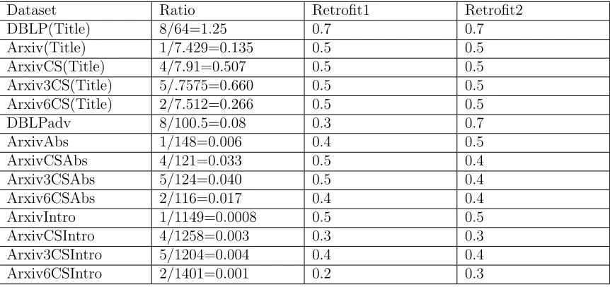
8 Hyper-parameterβtuning for the retrofit1. βwill determine how much weight to give to content or network information. Whenβ = 0, retrofit is biased towards content and will ignore network information. When β = 1, the retrofit will ignore the content information and give all weight to network information . . . 56
9 Hyper-parameter β tuning for retrofit2. β will determine how much weight to give to content or network information . . . 57
10 Additional CS datasets . . . 61
11 Experimental results for predicting the best possible value of β . . . . 62
12 Quality of the citation graph . . . 65
13 F1score of node2vec when the hyper-parameter p and q is varied. When p= 0.1, then q= (1−p) . . . 69
14 F1score of concatenated node2vec and PV-DBOW when the hyper-parameter pand q is varied. When p= 0.1, thenq = (1−p) . . . 70
16 PV-DBOW classification score using different vector dimensions . . . 72
17 Classification score after concatenating node2vec 15 and PV-DBOW
16. The dimension is doubled because half of the features are from
node2vec and the other half from PV-DBOW . . . 72
18 LDE Parameter Tuning forβ . . . 75
19 Classification Result when the content vector is obtained from PV-DM 78
CHAPTER 1
Introduction
Obtaining good representation of documents is crucial for different machine learning
tasks like classification, clustering and information retrieval. These tasks require
the input to be of short length vector. Recently, the most common method for
learning short length vector representation of text is Paragraph Vector (PV) [27].
Based on the distributed representation for words [31], PV proposed two models:
Paragraph Vector-Distributed Memory (PV-DM) and Paragraph Vector-Distributed
Bag of Words (PV-DBOW) with negative sampling and hierarchal softmax and the
input for these methods is only the text information as shown in Figure 1. These
methods assume that the documents are independent of each other.
Generally, documents are linked together in the form of hyperlinks in case of web
pages and citation in case of academic papers. Researchers tried to capture linkage
information while learning the representations like in node2vec [25]. These methods
ignore text information altogether during this process. The limitation of the methods
like PV-DBOW and node2vec is that they take information only from either the
content or network view alone. Intuitively, the vector obtained from using content
and network information together will give us a better vector representation.
Recently, the focus is shifted to learn multi-view representations [40]. For example,
learning document representation of academic papers from multiple views. We can
learn the representation using both the content and citation network by concatenating
1. INTRODUCTION
w1w2w3 p1
w3w1w5 p2
w1w6w3 p3
p1
p2
p3
PV-DBOW
vectors
node2vec
vectors
FIGURE 1: Learning Vector Representation from Content and Network
capturing different aspects of the documents and when combined will give a better
result for downstream tasks like classification than their single view counterparts.
In this thesis, we focus on improving the document representation of academic
papers using multiple views. Academic papers are more complex than plain texts
or networks. Papers contain text and are linked together through citations or
ref-erences. We can create a citation graph by connecting the paper together with the
papers that it is citing. The linkage is done based on the intuition that a paper cites
another paper which has a common topic or method. These network representation
learning methods, do not capture the content information, so they regard all the
pa-pers connected in the graph equal irrespective of their topics as shown in Figure 1.
For example, a paper in the domain of machine learning may cite papers related to
math and machine learning area. If we want similar papers, the network
represen-tation methods will consider papers belonging to math and machine learning equal
as it does not have the content information. Similarly, for methods like PV-DBOW
will output papers pertaining to the machine learning domain but it will ignore the
linkage of these papers with the math papers.
The contribution of this thesis is a multi-view based learning technique for
work, our method is applied as a post-processing step by running it on pre-trained
document vectors obtained from any method. The proposed method encourages the
new vectors to be similar to vectors which are linked together in the citation graph.
This process is fast and takes about 5 seconds for a graph of 10,000 documents and
vector length 100.
Our method is inspired by the existing method called Retrofit [22] for word
beddings. In retrofitting, they proposed a method in which they brought word
em-beddings closer together in the vector space based on the lexicons; meaning having
the same semantics. We modified the algorithm to extend it to document embeddings
and brought documents closer together based on the citation graph. Our experiments
show that our method improves the classification performance when compared with
existing methods.
1.1
Contributions
In this thesis we make the following contributions:
• Introduce a new algorithm for adding network information to the embeddings
obtained using content information in the form of retrofit.
• Show how the addition of network information improves the document
embed-ding through different methods.
• Analyze the reasons why when adding information from network and content
fails for some methods or datasets.
• Introduce a new dataset called Arxiv which contains both linkage and content
information for experimentation.
In the following sections, we will cover related work, problem statement, algorithm,
CHAPTER 2
Review of the Literature
This section will give a detailed analysis of the existing algorithms which try to
capture linkage information along with the content in the document embedding. For
each algorithm, we will explain the method and give a detailed description of the
dataset used for experimentation.
2.1
Concatenating Document and Network
Em-beddings
2.1.1
Learning Document Embedding
Paper [27] introduces Paragraph Vector (PV), an unsupervised algorithm that learns
fixed-length feature representation from variable length pieces of text such as
sen-tences, paragraphs or documents. The vectors are represented as dense vectors and
are trained to predict words in the document.
The PV have two models for learning document representation. We will explain
p1
...
government debt problems ...
p2
...
NLP analyses words in ...
p3
...
Basketball game was ...
p1
government debt problems
... ...
P(wt−1|p1)
P(wt|p1)
P(wt+1|p1)
FIGURE 3: PV-DBOW Overview
Paragraph Vector-Distributed Bag of Words (PV-DBOW) model since we used this
method in our experimentation
Figure 2 shows different paragraphs containing some text and each paragraph is
represented by a unique ID as p1, p2 or p3. The model will take paragraph ID and
content as input and will return the vector representation of all the paragraphs based
on content only.
Figure 3 gives an overview of the PV-DBOW model. For paragraphp1 we want to
maximize the probability of the words occurring in the paragraph with respect to all
the words in the vocabulary. This way the paragraph vectorp1 will capture semantic
representation of this paragraph based on the content information.
J(θ) = −1
Tlog(L(θ)) = − 1 T T X t=1 X −m<s<m j6=0
logP(wj|pt;θ) (1)
Equation 1 captures the vector representation of the paragraphs. θ are all the
variables that we want to optimize. T is the total number of documents in our
corpus. m is the window size and s is a word drawn randomly from that window. P
is the probability which we want to maximize when we have paragraph vector as an
input and want to predict the words present in that paragraph.
p(o|c) = exp u T ovc
P
w∈V exp(uTwvc)
(2)
The P(wj|pt;θ) is a softmax as defined in 2. In this case θ are the weight matrix
2. REVIEW OF THE LITERATURE 0 0 0 1 0 0
p1×t d
0.2 0.4 0.1 0.1 ... ... ... ... ... ... ... ... 0.2 0.4 0.1 0.1 ... 0.8 0.3 ... Dd×n v1×c n
WV×n
W vc
...
0.2 0.1 ...
SoftmaxP(w|p)
... 1 0 ... Truth one-hot vector for paragraph lookup column for paragraph embedding softmax Loss:
tilog(yi)
Backpropogation
Actual context word sampled randomly from the window
FIGURE 4: PV-DBOW Model
of hidden neurons or vector dimension and V is the total number of words in the
vocabulary. The vectorvcis obtained by multiplying one hot paragraph vectorpcwith
D. This will select a column in D and we represent this vector as vc. Similarly, uo
vector is obtained by the multiplication ofvc withW. uo is the vector representation
of the context word that we are trying to predict. To normalize the score, we will
multiply our paragraph vectorvc with all the word vectors uw in the vocabulary set
V.
Figure 4 explains the PV-DBOW model using graphical representation. In the
input, we pass one hot vector pt and multiply it with the weight matrix D. It will
select tth column of the weight matrix D and we will pass this column to the hidden
layer. The hidden layer is represented as a vector vc1×n where n is the number of
hidden neurons. We will then multiplyvcwith the words weight matrixW which will
give us uo vector containing the score in the output layer. Then we will pass uo to
the softmax which will give us a probability distribution of the words based on the
input vector. To calculate the loss we will use one hot vector representation of the
label word that we are trying to predict and multiply it with our softmax vector as
Dd×n v1×n Wn×V u1o×V y1×V c
weight
weight
input p1×d
t t1×V
label
FIGURE 5: Weight Update
respect to the weight matrixD.
SLoss=tilog(yi) (3)
Loss ∂D = Loss ∂y . ∂y ∂uo
.∂uo ∂vc
.∂vc
∂D (4)
Figure 5 gives a more abstract view of the PV-DBOW model and Equation 4 outlines
the series of partial derivative that we have to do to update the weight parameter D
where y is softmax, vc =Dpt and uo = vcW.
The problem with the above model is that for each iteration we will have to
calculate softmax and for its calculation we need to normalize the score for all the
words in the vocabulary which can be 105 to 107.
J(θ) = log σ(uovc) + K
X
k=1
Ej ∈P(w) [log σ(−ujvc)] (5)
To optimize this problem, the authors used Negative Sampling in which they tried
to maximize the probability of the input and context vector and tried to minimize
the probability betweenkrandom words drawn from the corpus and the input vector.
The equation 5 defines negative sampling where σ is a sigmoid function defined as 1
1 +e−x and P(w) = U(w)
3
4/Z is a unigram distribution for wordw in the training
2. REVIEW OF THE LITERATURE
Dataset Used
For Sentiment Analysis experimentation, they used Stanford Sentiment Treebank
Dataset [Sta]. This dataset contains 11855 sentences taken from movie review site
Rotten Tomatoes. Each sentence in the dataset has a label ranging from very positive
to very negative in the scale from 0.0 to 1.0. The sentences are further divided into
subphrases and each subphrase is labeled. Human annotators did the labeling, and
there are 239,232 labeled phrases in the dataset.
For experimenting with paragraphs and documents, they used IMDB [IMD] dataset
as a benchmark for sentiment analysis. The dataset contains 100,000 movie reviews
taken from IMDB. Each movie review consists of multiple sentences and reviews are
labeled as positive or negative.
For the information retrieval experiment they used a dataset of paragraphs
con-sisting of the first ten results returned by a search engine given each of 1,000,000 most
popular queries. To test vector representation, they created triplet of paragraphs such
that the two paragraphs are results of the same query and the third paragraph is a
randomly sampled paragraph from the rest of the collection.
During training, they learned the vector representation using the training dataset
only and then passed the representation to learn Logistic Regression classifier for the
prediction task. Once the model is trained, they tested it on the training dataset.
They first froze the model and obtained vector representation of the test sentences
and then passed this representation to the trained Logistic Regression model.
Sentiment Analysis
For sentiment analysis experiment with Stanford Sentiment dataset, they used two
approaches for classification [27]. First, they proposed a 5-way fine-grained
classifi-cation task where the labels are from very negative, negative, neutral, positive and
labels are either positive or negative. Each phrase is treated as an independent
sen-tence, and after learning vector representation, they are fed into logistic regression
to predict the movie rating. The window size used is 8, and vector representation
has a dimension of 400. The results show that their method outperforms the other
baseline methods like the bag of words, bag of n-words or Naive Bayes by relative
improvement of 16% in terms of error rates. Error rates calculates the percentage
error by subtracting the original value with the predicted value and dividing it by the
original value.
In the case of IMDB dataset, they learned vector representation through a neural
network with one hidden layer with 50 units and a logistic classifier to learn to predict
the sentiment. They used the same hyperparameters as they used in Stanford Dataset
except the window size is 10. The result shows that the bag of words performed better
than in the previous experiment because of long documents. Overall, paragraph vector
again outperforms the other methods as it achieves 7.42% error rate which is the least
when compared with the other techniques [27].
Information Retrieval
The objective of this experiment is to find which of the three paragraphs are from
the same query in the dataset they created. To achieve this, they used paragraph
vectors and computed distances between them. A better representation is one, which
produces a small distance for pairs of paragraphs of the same query and a large
distance for a paragraph from a different query. They used bag of words, bag of
bigrams and averaging word vectors as a benchmark. They recorded the number
of times where each method produces smaller distance for the paragraphs from the
same query and error was made if the method does not provide a desirable result.
The result showed that Paragraph Vector gave 32% relative improvement in terms
2. REVIEW OF THE LITERATURE
semantics of the text.
Conclusion
This paper introduced an unsupervised learning algorithm that learns vector
rep-resentation for a variable length of texts. In this method, it is assumed that
docu-ments(phrases) are independent of each other, but in the real world, it is the opposite.
Documents are linked with each other in the form of links or citation in case of web
pages or academic papers respectively. The document embeddings are not able to
capture this linkage information by default; as a result, this method ignores this
link-age information altogether. In the experimentation, it is also advised to use PV-DM
with concatenating vectors and a window size of 5 to 12.
2.1.2
Learning Network Embedding using Node2vec
Paper [25] proposes an algorithm for learning continuous feature representation for
nodes in a network by mapping them to low dimensional space of features that
max-imize the likelihood of preserving network neighborhoods of nodes.
Algorithm
This algorithm uses network information to learn the feature embeddings. Let u be
the source node and Ns(u) be the neighbourhood of nodes connected with u using
sampling strategy like DeepWalk [33] or Node2Vec [25]. The set of sequence of nodes
produced from this sampling strategy can be considered as a sentence and each node
in the sequence as a word as shown in Figure 6. Then we can use a model similar
to the skip-gram [31] to learn the feature embedding ofu by predicting it’s neighbor
node in the output.
The process of learning the feature embedding is the same as described in the
n1
n2
n3
Ns(n2) = {...n1, ni, n3, ny, ....}
s=Sampling Strategy
n2
n1 n3 ni
... ...
P(nt−1|u)
P(nt|u)
P(nt+1|u) Network
network neighborhood of source node d2
FIGURE 6: lnput to node2vec
Output Layer Hidden Layer Input Layer H1 H2 Hd
FT d×V
u1
u2
u3
FV×d
uV u1×V n1 n2 n3 nV
h1×d
v1×V
2. REVIEW OF THE LITERATURE
6 and shown in Figure 7.
maxf
X
u ∈ V
log P (Ns(u) | f(u)) (6)
where f is a matrix of size |V| ×d and V is the total number of nodes and d is
the number of hidden neurons.
In node2vec, they use 2nd order random walk algorithm to find the neighboring
nodes in the network. They define two hyperparameters p and q which tries to find
nodes sharing a similar community and similar structure through breadth-first and
depth-first search respectively. Figure 8 describes this concept in more detail.
u1
s1 s2
s3 s4
u2
s5 s6
s7 s8
Depth First
Breadth First
FIGURE 8: Graph Structure in node2vec
If we want to find nodes belonging to the similar community as the source node
u, we will increase the value of q, so that breadth-first search is given more weight.
Similarly to find nodes sharing a similar structure, we will increase the value of pto
promote depth-first search in the random walk.
Dataset Used
This paper uses four different datasets for experimentation. For learning feature
representation for a node in a network, they used Les Miserable Network [26], where
nodes correspond to characters in the novel and edges connect coappearing characters.
This network has 77 nodes and 254 edges. In multi-label classification experiments,
has 10,312 nodes and 333,983 edges. Second is Protein-Protein Interaction [PPI] [34]
which contains subgraph of the PPI network of Homo Sapiens. This network has
3,890 edges and 76,584 nodes. Lastly, they used Wikipedia [wik] dataset containing
co-occurrence network of words appearing in the first million bytes of the Wikipedia
dump. This network has 4,777 nodes and 184,812 edges.
For link prediction experiment, two additional datasets are used; Facebook [28]
and arXiv ASTRO-PH [arx]. In facebook, nodes represented users and edges
repre-sented friendship relation between them. The network has 4,0396 nodes and 88,234
edges. ArXiv is a collection of network generated from papers submitted to the
e-print arXiv. In this dataset, nodes represent scientists, and an edge is present if two
nodes co-authored in a paper. This network has 18,722 nodes and 198,110 edges.
Learning Edge Features
For experimentation, they used node2vec to learn feature representation for nodes in
a network. They observed that Breath First Search (BFS) and Depth First Search
(DFS) strategies both represent extreme ends on the spectrum of embedding nodes
based on the principle of homophily (similar network communities) and structural
equivalence (structural role of nodes). They demonstrated that node2vec could
ob-tain embeddings that obey both the principles. They set d = 16 and ran node2vec
on the Les Miserables dataset. Then the feature representations were clustered using
k-means. Then they visualize the original network in two dimensions with nodes now
assigned colors based on their clusters. They set p= 1 andq = 0.5 to capture nodes
which interact more often with each other hence same community. This
character-ization relates to homophily. To discover structure equivalence they set p = 1 and
q = 2 as node2vec hyperparameters. This setting captured nodes which have the
2. REVIEW OF THE LITERATURE
Multi-label Classification
In multi-label classification experiment, every node was assigned one or more labels
from a finite set. During training, they used a certain fraction of nodes and all their
labels. The objective of the experiment is to predict the labels for the remaining
nodes. They used BlogCatalog, PPI and Wikipedia dataset for this experiment.
They compared node2vec against Spectral clustering [38], DeepWalk [33] and Line
[36] for evaluating the performance. The node features were passed to a one-vs-rest
logistic regression classifier with L2 regularization. They used Macro-F1score for
comparing the performance. Node2vec outperformed other methods because of the
added flexibility in the algorithm by fixing hyperparameters p and q to low values.
This setting enabled node2vec to capture homophily and structural equivalence in
the network.
Link Prediction
In link prediction, first, they removed 50% of edges randomly from the network while
making sure that the residual network remains connected after these edges are
re-moved. The objective of this experiment is to predict the missing edges. They used
Facebook, PPI and arXiv dataset for this experiment. They compared node2vec and
other benchmarking algorithms with some popular heuristic scores that achieve good
performance in link prediction. Node2vec outperformed DeepWalk and Line in all
networks with gains up to 3.8% and 6.5% respectively using AUC scores.
Conclusion
This paper focuses on learning feature representation of a network as a search based
optimization problem. It explains the classic search as a trade-off between exploration
and exploitation. It shows that BFS can explore only limited neighbourhoods and it is
X
MV xV WV×k
Hk×ft
prob that di walk to dj di
dj
Mij
X
Fft×V
FIGURE 9: TADW Model
freely explore the network and can discover homophilous communities in the network.
It is assumed while factorizing the likelihood that the observed nodes are independent
of each other while learning the feature representation. Just like in the PV-DBOW
model, the context nodes are considered to have no relationship with each other. In
this algorithm, the content of the nodes is totally ignored. Therefore, the produced
representation of the documents does not capture the content of the document.
Concatenating PV-DBOW and Node2vec Embeddings
To capture both the content and link information for learning document embedding,
we can concatenate the embeddings produced from the above methods for the
down-stream tasks like classification. This method will not capture the complex relationship
between the documents regarding content and linkage. After concatenation, the
vec-tor dimension will double, and we can use dimensionality reduction methods like
PCA [41] to reduce the dimensions. During this process, we will lose some feature
information which might downgrade our classification result.
2.2
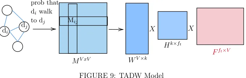
Text Associated DeepWalk (TADW)
Paper [42] proposes an algorithm to include text information to the network
2. REVIEW OF THE LITERATURE
Algorithm
TADW algorithm tries to capture the linkage and content information together when
learning the document representation. First, the content information is converted
into vector representation using TF-IDF matrix or binary vector and represented as
Fft×V where ft is the number of dimensions we want to represent each word in the
vocabularyV. Then, the model will construct matrixMV×V where each entryMij is
a probability of walking from the documentdi todj based on the sequence generated
using sampling strategy like DeepWalk [33] as shown in Figure 9.
The goal is to approximate matrix WV×k and Hk×ft where k is the dimension
of the vector we want to learn using matrix M and F through inductive matrix
factorization [32].
minW,H
X
i,j∈
Mij − WTHT
2
+ λ
2 ||W|| 2
F +||H||
2
F
(7)
The equation 7 shows that we try to approximate the matrixM through inductive
matrix factorization. We try to learn the matrixW andHand use the feature matrix
F to obtain better representation. λ is a regularizer which prevents the model from
overfitting. Computation of M is very expensive and can take O |V|2
times where
V is the total number of documents [42].
Dataset Used
For experimentation, they used three datasets:
• Cora: It contains 2,708 machine learning documents with 5,429 citation links.
Each document is represented by a binary vector of 1,433 dimensions indicating
the presence of the corresponding word
indicates the presence of the word
• Wiki: This dataset contains 2,405 documents with 17,981 links. The document
is represented as TD-IDF matrix with 4,973 columns
Experimentation
As an input for the experimentation, they reduced the vector dimensions by
us-ing SVD [23] decomposition and obtained a vector dimension of 200 for the TADW
method. For classification, they used an SVM classifier. While training they used
one-vs-rest classifier for each class and selected the class which has the maximum score.
The experimentation result showed that TADW consistently performs much better
than the other baseline methods and can also work well when there is a significant
amount of noise in the graph.
Conclusion
This paper gives a proof that the DeepWalk algorithm is equivalent to the matrix
factorization and using this concept they tried to incorporate the text information
in the network representation learning method DeepWalk. The proposed method
does not support online and distributed learning for large scale networks. It is also
computationally expensive as the procedure of computing M takes O|V2| , TADW,
takes into account both the text and network information for learning the document
embedding. Instead of just concatenating the vectors, it proposed a method of jointly
modeling feature combination via matrix factorization. As a result, for paper
similar-ity experiment they showed that when finding similar papers related to the category
of theory. TADW found all papers belonging to the same topic whereas DeepWalk
returned paper belonging to different class labels. Though the original query paper
cited all the returned papers. This was because DeepWalk considered all the papers
2. REVIEW OF THE LITERATURE
This experiment proved that adding text information to the network embedding will
learn better representation.
2.3
Linked Document Embedding for
Classifica-tion
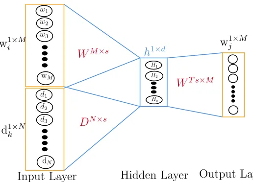
Paper [39] introduces an algorithm which tries to incorporate the linkage and
la-bel information between the documents along with the content information to the
document embeddings.
Algorithm
In the algorithm, they try to capture the linkage and content information together
while learning the document embedding. The algorithm consists of two parts:
1. learning word-word embedding for the documents using content only
2. learning document-document embeddings using the network only
maxW D 1 |P|
X
wi,wj,dk ∈ P
log P (wj | wi, dk) (8)
In the first part, for each target word wi they extract c neighbours as wj based
on the window size. They also store the information from where this word was
extracted by adding document ID. Together the pair of words and the document form
a triplet (wi,wj, dj) and stored in the set P. Objective function 8 tries to maximize
the probability of the neighbor words wj given the target wordwi and the document
vectordk. WM×s andDN×s are the weight matrices that we want to learn. M is the
Output Layer Hidden Layer Input Layer H1 H2 Hs
WT s×M
w1
w2
w3
WM×s
wM
w1j×M
d1
d2
d3 DN×s
dN w1i×M
d1k×N
h1×d
FIGURE 10: Learning Document Representation using Content Information
Output Layer Hidden Layer Input Layer H1 H2 Hs
DT s×N
d1j×N d1
d2
d3
DN×s
dN d1i×N
h1×d
FIGURE 11: Learning Document Representation using Network Information
in the corpus. s is the dimension of the vectors. Figure 10 shows an outline of the
model. maxD 1 |E| N X i=1 X
j:eij=1
log P (dj | di) (9)
In the second part, they learn the document embeddings using the graph G(N, E)
whereN is a total number of documents andE represents an edge betweendi anddj.
The objective is to maximize the probability of the neighbouring nodes in G when
the source node di is given. The equation 9 defines this concept where E is the set
containing document-document pair based on citation information and eij = 1 only
2. REVIEW OF THE LITERATURE
1 |P|
X
(wi,wj,dk)∈P
log P (wj|wi, dk) + 1 |E| N X i=1 X
j:eij=1
log P (dj|di) −γ(W, D) (10)
Equation 10 gives an overview of the model. In the first part, we try to learn the
document representation using only the content information, and in the second part,
we use network information to learn the document representation. γ is a regularizer
so that the model does not overfit.
For experimentation, we use source code build by Yi Zhang as the authors did
not provide the code.
Dataset Used
For experimentation, they used two datasets DBLP and BlogCatalog. They extracted
only title and abstract as content information for the DBLP dataset and chose six
categories for the experimentation. Each group consisted of 2,550 samples and in
total 15,300 documents were used with 36,359 total links.
In the case of the BlogCatalog dataset, they used text description in each blog
as the content and determined links according to the related blogs mentioned by the
website. They also assumed the presence of the link between two blogs if the authors
of the blogs followed each other. In total, the dataset contained 62,652 documents
with 378,161 links. This dataset is unbalanced.
Experimentation
For experimentation, they used F1micro and F1macro as an evaluation metrics.
They compared the proposed method with the other existing methods like PV-DM,
PV-DBOW, and PTE [35]. Their experiment consisted of two-phase; the
phase, they used the whole dataset to train word embeddings and document
embed-dings. Label information of the training data is also used for learning whereas the
labels of the testing data are not included during the learning phase. The used
di-mension size of 100 and window size of 7 and the number of negative samples equal
to 7.
Conclusion
The result of experimentation proves that the inclusion of link information to the
document embeddings will improve the classification result. They also
experimen-tally showed the effect of link density on the classification task, and as the density
increases, the classification accuracy also increased. In this paper, they did not test
the embeddings against other baseline experiment methods like document
recommen-dation or embedding visualization. In the proposed method, it is also assumed that
the weight of links is uniform for all the edges. In the real world, it is not the case,
as the documents might have weighted edges between them in the form of page rank
CHAPTER 3
Retrofit Algorithm
In this section, we will formally define the problem statement and explain our
algo-rithm in detail.
3.1
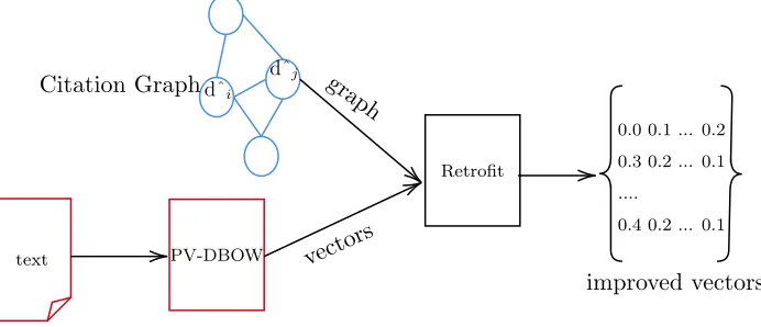
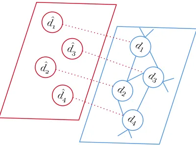
Problem Statement
Given the content based embedding of the document dˆi, we want to learn the new
embedding of document di such that it is close to its original embedding and also to
the embeddings of the documents that it is linked with.
dˆi
dˆj
PV-DBOW text
Retrofit
vectors graph Citation Graph
0.0 0.1 ... 0.2
0.3 0.2 ... 0.1
....
0.4 0.2 ... 0.1
improved vectors
ˆ d ˆ d ˆ d ˆ d d1 d2 d3 d 4
FIGURE 13: Retrofit Algorithm
3.2
Proposed Algorithm
The proposed method Retrofit will try to bring document embeddings close together
based on citation and network information. The Retrofit takes vectors produced from
PV-DBOW [27] as an input. The vectors from PV-DBOW lack knowledge from the
citation graph. The Retrofit will also take the citation graph as input and will add
network information to the PV-DBOW vectors as shown in Figure 12.
Let V ={d1, d2, ..., dn} be a set of n documents and G be a graph that captures
citation links between the documents in V. We represent G as an undirected graph
(V, E) with one vertex for each document type and edge (di, dj) ∈ E ⊂ V × V
indicating citation relationship between the two documents.
LetDˆ = (dˆ1,dˆ2, ...,dˆn)T be the matrix for the vector representation of each
doc-ument d iˆ ∈ <k for eachd
i ∈ V learned using standard document embedding
repre-sentation methods wherek is the dimension of the vector. Our aim is to learn matrix
D= (d1,d2, ...,dn) such that di is close to ˆdi and to the citing documents in G.
The objective is to minimize the distance between the documentdi, and the edges
it is connected with in the citation graph (di, dj) ∈ E. The document ˆdi represents
the original embeddings, and we want to bring the retrofitted embedding close to
the original embedding and to its neighbor as shown in Figure 13. Since there is no
3. RETROFIT ALGORITHM
to solve this problem. This is because D can contain 10,000,000 documents and a
dense 100 dimensional vector can represent each document. For finding a closed-form
solution, we need to store DDT matrix which will require 1×10¹⁰ floating point
numbers. At 8 bytes per number, this comes to 80GB which is impractical to store
on anything but a supercomputer. Furthermore, computing inverse of this matrix
would also be very expensive. We have two variants of the retrofit algorithm called
retrofit1 and retrofit2. The difference between these two methods is how we add the
citation information to the document embeddings.
J(D) = N
X
i=1
(1 − β)|| di − dˆi ||
2
2 +β
X
(i,j) ∈ E
||di − dj ||22
(1)
Retrofit1
Equation 1 defines the objective function of retrofit1 where β is a hyperparameter.
The boldface lower case letters represent vector representation of the documents. J in
Equation 1 is a convex in D [22]. The hyperparameterβ controls the relative strength
of association in Equation 1. This objective function gives more weight to nodes with
high degrees. The weight beta loops over the links and adds them to the document
vector. This weight controls how much we want the document embedding to come
close to its neighbors. This approach is modular meaning it can be applied to any
document vector representation obtained from any model. We use Squared Euclidean
distance (SED) [22] to define the distance between the pair of vectors. First, we shall
define the Euclidean distance [21] betweendi anddˆiin Equation 2. kis the dimension
of the vector.
||di−dˆi ||2 =
q
Equation 2 can be further simplified to 3.
||di−dˆi||2 =
v u u t k X x=1
dix−dˆix
2
(3)
We use SED to remove the square root and make calculations less expensive.
SED is a smooth and strictly convex function of the two points and is preferred
in optimization theory [20]. Equation 4 measures the similarity between retrofitted
embedding di and initial content-based vectordˆi using SED.
||di−dˆi||22 =
k
X
x=1
dix−dˆix
2
(4)
The objective function 1 refers to the task of minimizing the distance of
docu-ment vectors based on content and citation network. The derivative of the objective
function will give us an updating equation for the change in vector di to reduce the
distance between the content based vector ˆdi and the citing papers dj , ∀j where
(i, j) ∈ E [24]. This derivative specifies how much change in the input will scale to
the change in the output. The derivative is useful in determining the change in di to
make a small improvement in the output. Since our objective function has multiple
variables, we take the partial derivative to measure the change concerning the
spe-cific component. Now we take the partial derivative of our objective function 1 with
respect to di and obtain the updating equation for the new vector di.
∂J(D) ∂di
= N
X
i=1
(1−β)|| di − dˆi ||22 +β
X
(i,j) ∈ E
||di − dj ||22
(5)
First we take the derivative of ||di − dˆi||22 and
X
(i,j) ∈ E
3. RETROFIT ALGORITHM
di
∂J(D) ∂di
= N
X
i=1
(1−β)
∂ ∂di
|| di − dˆi ||22 +β ∂ ∂di
X
(i,j) ∈ E
||di − dj ||22
(6)
We will use chain rule [19] to take the derivative of || di − dˆi ||22 which can be
written ash(g(x)) where his the ||2
2 as defined in 4 and g(x) =di−dˆi. First we will
take the derivative of the ||224
∂J(D) ∂di
= N
X
i=1
[2(1−β)di − ˆdi
∂
∂di
di − dˆi
+ 2β X
(i,j) ∈ E
(di − dj )
∂ ∂di
(di − dj )]
(7)
and then the derivative of g(x).
∂J(D) ∂di
= 2∗(1−β)di−dˆi
(1) + 2β X
(i,j) ∈ E
(di−dj) (8)
Now lets suppose ∂J(D) ∂di
= 0:
(1−β)(di)−(1−β)
ˆ di
+ β X
(i,j) ∈ E
(di)−β
X
(i,j) ∈ E
(dj) = 0 (9)
We will move all thedi terms to one side and all the other terms to another side.
(1−β)(di) + β
X
(i,j) ∈ E
(di) =β
X
(i,j) ∈ E
(dj) + (1−β)
ˆ di
(10)
Then we will takedias common and divide its coefficient where
X
(i,j)∈E
di=deg(di)(di)
di =
βP
(i,j) ∈ E(dj) + (1−β)
ˆ di
(1−β) + β×deg(di)
Input Output f(x01, x02, x03, ..., x0n) x11 f(x11, x02, x03, ..., x0n) x12 f(x1
1, x12, x03, ..., x0n) x13
... ...
f(xm1 +1, xm2 +1, x3m+1, ..., xmn) xm3+1
TABLE 1: Example of the Gauss-Seidel method. m is the number of step. The complete table shows one iteration. For each step in a single iteration, we will always use the latest value
Equation 11 is an online update equation we use in each iteration to obtain the
vector representation of di. For updating di, we use an iterative updating method as
used in [20]. In [20] they try to build a graph for data points containing labeled and
unlabeled points. Known labels are used to propagate information in the graph in
order to label all the nodes using edges as a similarity. They also used an iterative
updating method to update the label information in the graph. Our approach uses
Gauss-Seidel as implemented in [20] to solve the system of linear equations. The
system of linear equations is the updating equation for each di in D. The
Gauss-Seidel method works by using the latest value in D for each iteration. For example,
x= (x1, x2, ....xn) is the true solution of x. If xm1+1 is better then xm to approximate
x2, x3, ..., xn, then we will use the new valuex1m+1rather thanxm. mis the number of
steps. For findingxm2 +1, instead of using the old value xm
1 , we will usex
m+1
1 and the
subsequent old values xm
3 , xm4 , ...., xmn. Similarly, for finding xm3+1, we will use xm1+1
and xm2+1 and the subsequent x4m, xm5 , ..., xmn. Table 1 shows how the latest value ofx
3. RETROFIT ALGORITHM
Algorithm 1: Retrofit1
Result: Adds citation information to the content based vector
representation of documents in the matrixDˆ
Input : ˆD,G= (V, E),iterations, β
Output: D
1 D =Dˆ
2 for iter=0 to iterationsdo
3 foreach di in D do
4 vi = (1-β)∗deg(di) * dˆi
5 foreach dj in E(di) do
6 vi = vi+β *dj
7 di = vi / (2*deg(di))
8 end
9 end
10 end
Algorithm 1 links the objective function 1 and shows how we implemented the
updating step 11 in the code. In algorithm 1Dˆ is a matrix representing content based
vector representation of N documents. E(di) will give us a list of all the documents
that are connected with di in the network graph. Iteration is a hyper-parameter
which will determine how many times we want to repeat this process. deg(di) is the
degree of the documentdi in the citation graph. Line 4 of the algorithm 1 will add the
information from content based embedding and line 6 will add information from the
network view. Line 7 takes the average of the content and network based embedding
for each dj. The computational complexity of retrofit1 is (tn) where t is the total
number of neighbours and n is the total number of documents in the dataset.
def retrofit1(D_hat, G, iterations, beta):
for it in iterations:
for d_i in D:
numNeighbours = len(G(d_i))
if numNeighbours == 0:
continue
v_i = (1-beta)*numNeighbours*D_hat[d_i]
for d_j in G(d_i):
v_i += beta*D[d_j]
D[d_i] = v_i / (2*numNeighbours)
return D
Listing 3.1: Retrofit1 Code. Complete code can be found at https://github.com/
ZeeshanMansoor260/Masters/blob/master/Retrofit/retrofit_document.py
Code 3.1 shows the implementation of retrofit1 in Python. The complete code can
be accessed at https://github.com/ZeeshanMansoor260/Masters/blob/master/
Retrofit/retrofit_document.pyand we originally obtained this code from [22]. G
is the citation graph and G(di) will return the list of documents that are connected
with di in the network.
Retrofit2
J(D) = N
X
i=1
(1 − β)||di − dˆi ||
2
2 +β|| di −
1 deg(di)
X
(i,j) ∈ E dj ||22
(12)
Another variant of the retrofit algorithm called retrofit2 is defined in 12. Retrofit2
first takes an average of all the documents that it is citing and then add that to the
content using β as the weight for network information and deg(di) is the degree of
the document di. We use SED 4 to calculate the distance between the embeddings.
For retrofit2, we will again take the first derivative of the objective function 12
3. RETROFIT ALGORITHM
retrofit1.
The objective function for retrofit 2 is defined as:
J(D) = N
X
i=1
(1−β) || di − dˆi ||22 +β|| di −
1 deg(di)
X
(i,j) ∈ E dj ||22
We take the partial derivative of J(D) with respect to di
∂J(D) ∂di
= N
X
i=1
(1−β)|| di − dˆi ||22 +β|| di −
1 deg(di)
X
(i,j) ∈ E dj ||22
(13)
Now we take the derivative of || di − ˆdi ||22 and ||di −
1 deg(di)
X
(i,j)∈ E
dj ||22
∂J(D) ∂di
= N
X
i=1
(1−β)
∂ ∂di
|| di − ˆdi ||22 +β ∂ ∂di
||di −
∂ deg(di)
X
(i,j) ∈ E
dj ||22
(14)
Again||di − ˆdi ||22can be considered ash(g(x)) and we will apply chain rule to take
it derivation. First we take the derivative of the||22 4.
∂J(D) ∂di
= N
X
i=1
[2(1−β) di − dˆi
∂
∂di
di − ˆdi
+2β
di −
1 deg(di)
X
(i,j) ∈ E dj
∂ ∂di
di −
1 deg(di)
X
(i,j) ∈ E dj
]
Then we take the derivative of the g(x)
∂J(D) ∂di
= 2∗(1−β)di−dˆi
(1) + 2β
di −
1 deg(di)
X
(i,j) ∈ E dj
After that we will cancel out 2
∂J(D) ∂di
= (1−β)di−dˆi
+ β
di −
1 deg(di)
X
(i,j)∈ E dj
(16)
Now lets suppose ∂J(D) ∂di
= 0
(1−β)(di) −(1−β)
ˆ di
+ β(di) −
β deg(di)
X
(i,j) ∈ E
dj = 0 (17)
We will move all thedi terms to one side
(1−β)(di) + β(di) = (1−β)
ˆ di
+ β
deg(di)
X
(i,j) ∈ E dj
After simplifying the left hand side will obtain the following update equation
di = (1−β)
ˆ di
+ β
deg(di)
X
(i,j) ∈ E
dj (18)
3. RETROFIT ALGORITHM
will use the latest vectors in D and after 10 iterations it will converge [22].
Algorithm 2: Retrofit2
Result: Adds citation information to the content based vector
representation of documents in the matrixDˆ
Input : ˆD,G= (V, E),iterations, β
Output: D
1 D =Dˆ
2 for iter=0 to iterationsdo
3 foreach di in D do
4 netvec =0
5 foreach dj in E(di) do
6 netvec += dj
7 end
8 netvec =netvec/ deg(di)
9 di = (1−β) ˆdi +β(netvec)
10 end
11 end
We will now link algorithm 2 with the update equation 19.
di = (1−β)
ˆ di
+ β
deg(di)
X
(i,j) ∈ E
dj (19)
In 19 (1−β)ˆdiis obtaining information from the content view and implemented in
line 9 of the algorithm 2. β deg(di)
X
(i,j) ∈ E
dj is getting information from the network
view and implemented from line 5 to 8 of the algorithm 2. Information from both
the views is then combined in line 9 as shown in the algorithm 2. The computational
complexity of retrofit2 is (tn) where t is the total number of neighbours and n is the
def retrofit2(D_hat, G, iterations, beta):
D = D_hat
for it in iterations:
for d_i in D:
numNeighbours = len(G(d_i))
if numNeighbours == 0:
continue
netvec = np.zeros(D.dim)
for d_j in G(d_i):
netvec += beta*D[d_j]
netvec = netvec / (numNeighbours)
D[d_i] = (1-beta)*numNeighbours*D_hat[d_i] + netvec
return D
Listing 3.2: Retrofit2 Code
The code 3.2 is the implementation of the retrofit2 algorithm in Python. The
complete code can be found athttps://github.com/ZeeshanMansoor260/Masters/
blob/master/Retrofit/retrofit_document_adv.py. G is the citation graph and
G(di) will return the list of documents that di is connected with in the network.
3.2.1
Code Flow
This section will explain the flow of code from the point of learning embeddings
from text to classifying evaluation. The underlying retrofitting code is obtained from
[22]. We converted the code from word embeddings to the document embeddings.
The code architecture is decoupled into several components. A single program called
Run.py launches all components. Upon running this file, it will trigger the content
based embedding learning module. This module uses PV-DBOW to learn vector
3. RETROFIT ALGORITHM
to obtain the linkage information from the network. The information from both the
network and the content will then be passed to the retrofit module. The retrofit
will try to add the linkage information to the content based embeddings using the
algorithms defined above. Once the embeddings are retrofitted, then they will be
passed to the classification and visualization module for evaluation. This code can
CHAPTER 4
Datasets
This section will explain the four datasets we used for our experimentation in detail.
4.1
DBLP
First, we will outline the details regarding the Digital Bibliography and Library
Project DBLP dataset [dbl]. For initial experimentation, we used a small dataset
and classified the papers based on the conferences. We extracted documents from
DBLP which is a computer science bibliography provided by the University of Trier
in Germany. From DBLP published venue metadata, we can find papers that belong
to specific conferences. We used three popular conferences: VLDB, SIGMOD, and
ICSE. The details of the three conferences are listed below:
• VLDB: The International Conference on very Large Databases constitutes of
research papers focusing on research in the field of database management [vld].
• ACM SIGMOD: The International Conference on Management of Data [sig]
contains research papers focusing on principles, techniques and applications of
database management systems and data management technology.
• ICSE: The International Conference on Software Engineering [ics] comprises
of all the papers that contain most recent innovation, trends, experiences and
4. DATASETS
FIGURE 14: Document size and classes distribution in the DBLP dataset
In the rest of our discussion, we will use DBLP to refer to the combined dataset
consisting of the above three conferences.
The DBLP dataset consisted of title only, and the average text length is 6.4 words
per document. For experimentation, we wanted to have more content and see the
effect of adding network information to the vector representation consisting of content
information only. We combined the DBLP dataset with the Aminer [37] to increase
the content. The Aminer dataset has more details like title, abstract, authors and
references. This dataset contains citation information extracted from the Microsoft
Academic Graph (MAG), ACM and DBLP. We used version 10 of the Aminer dataset
which includes 3 million papers. Then we merged the DBLP dataset with the Aminer
dataset using the title to link between these two datasets. Once connected, we added
abstract information to the DBLP dataset and called this dataset as DBLPadv. We
were able to link 6704 documents, and the average text length increased to 100.5.
Figure 14 shows the document size and label statistics of the DBLP dataset. We
can see that all the 3 classes are uniformly distributed and most of the documents
have title length of 6.4.
Figure 15 shows the distribution of words and labels for DBLPadv dataset. In
FIGURE 15: Document size and classes distribution in the DBLPadv dataset
class distribution of the ICSE documents has decreased. This is because we could not
link some of the documents with the Aminer dataset when trying to extract abstract
information.
4.2
ArXiv
The following sections explain how we created the arXiv [arx] dataset and the method
we used for adding reference information.
4.2.1
ArXiv Content Extraction
arXiv [arx] is an open-access containing papers in the domain of Physics,
Mathe-matics, Computer Science, Quantitative Biology, Quantitative Finance, Statistics,
Electrical Engineering, and Economics. arXiv dataset stores the source code of the
documents in the form of Latex format.
We are interested in the source code as it gave us more freedom to extract the
different type of information like titles or abstract from each document. We
down-loaded the Latex files from 1997 to 2018 from the Amazon S3 servers. Each tar file
4. DATASETS
Latex Files
bash
convert multiple latex code files to one file
Latex Code
Python extraction
id title id abstract id sections
FIGURE 16: arXiv Extract FlowChart
complete dataset is approximately 600GB.
The tar files are named using the following convention:
yymm.chunk
where yy represents the year, mm represents the month in which the paper was
published and chunk as the number of the tar file. For example, the tar file named
1401.01 means that the papers in this tar were published in January 2014. The chunk
01 means the number of this tar file as there are several chunks of each tar files.
Once extracted, each document’s filename is it’s paperID, and the complete source
code is present inside that file. For papers which contains several files, the directory’s
name is the paperID, and all of its files are present in that directory.
Initially, to extract title and paperID from this dataset, we developed a bash
script in Linux. A bash script is a text file which can contain Linux commands and
will execute them when running. This bash script will search for the title in all the
files using an awk command and stores it in another file containing paperID and
title only. Similarly, we extended this method for extracting abstract, introduction
section, middle section and last section from all the papers and linked them with
their paperIDs. This method we found to be very slow and subsequently, we modified
the bash scripts such that, it only finds the tex file which contains the main tex code
for all the documents and copies it to another directory. Then a Python script will
Title Extraction
\title [class] % comments { title \textbf{ something to bold } remaining title \}
FIGURE 17: Title Format in Latex
Title Example
Scenario 1: \title {Numerical Methods for Quasi-Periodic Incident Fields Scattered by Locally Perturbed Periodic Surfaces}
Scenario 2: { \textbf{On the diameter and incidence energy of iterated total graphs}}
Scenario 3: \title{Dynamics of Nonlinear Random Walks on Complex Net-works \thanks{Submitted to the editors DATE.
FIGURE 18: Different scenarios for extracting title
using regex expressions and store them in a separate file according to the following
format
PaperID Title
Within the title, there might be other latex tags which we do not want to acquire
like comments or class as shown in figure 17. To counter that, we used a stack to
identify the beginning of the title using {. Whenever we saw { we increased our
stack and whenever we saw } we decreased our stack until it is empty. As a result,
we were able to capture the title of the document only and ignore other information
like comments. For example the figure 18 shows different scenarios from which we
need to extract title. Scenario 1 is the most straightforward situation. Using regex
expression, we detect \title and add { to the stack and start reading. When we see
} we remove it from the stack, and if the stack is empty, we stop reading. Scenario
2 is more complicated. Instead of \title, it uses \textbf, and we also search for this
alternative. Situation 3 is the most complicated. It does not have a} bracket at the