Retrieval Term Prediction Using Deep Learning Methods
Qing Ma† Ibuki Tanigawa† Masaki Murata‡
†Department of Applied Mathematics and Informatics, Ryukoku University ‡Department of Information and Electronics, Tottori University
Abstract
This paper presents methods to predict re-trieval terms from relevant/surrounding words or descriptive texts in Japanese by using deep learning methods, which are implemented with stacked denoising autoencoders (SdA), as well as deep belief networks (DBN). To determine the effectiveness of using DBN and SdA for this task, we compare them with conventional machine learning methods, i.e., multi-layer perceptron (MLP) and sup-port vector machines (SVM). We also com-pare their performance in case of using three regularization methods, the weight decay (L2 regularization), sparsity (L1 regularization), and dropout regularization. The experimen-tal results show that (1) adding automatically gathered unlabeled data to the labeled data for unsupervised learning is an effective measure for improving the prediction precision, and (2) using DBN or SdA results in higher prediction precision than using SVM or MLP, whether or not regularization methods are used.
1 Introduction
Existing Web search engines have very high re-trieval performance as long as the proper rere-trieval terms are input. However, many people, particularly children, seniors, and foreigners, have difficulty de-ciding on the proper retrieval terms for represent-ing the retrieval objects,1 especially in searches
1
For example, according to a questionnaire admin-istered by Microsoft in 2010, about 60% of users had difficulty deciding on the proper retrieval terms. (http://www.garbagenews.net/archives/1466626.html)
(http://news.mynavi.jp/news/2010/07/05/028/)
related to technical fields. Support systems are in place for search engine users that show suit-able retrieval term candidates when clues such as their descriptive texts or relevant/surrounding words are given by the users. For example, when the relevant/surrounding words “computer”, “previous state”, and “return” are given by users, “system re-store” is predicted by the systems as a retrieval term candidate. It is therefore necessary to develop var-ious domain-specific information retrieval support systems that can predict suitable retrieval terms from relevant/surrounding words or descriptive texts in Japanese.
In recent years, on the other hand, deep learn-ing/neural network techniques have attracted a great deal of attention in various fields and have been suc-cessfully applied not only in speech recognition (Li et al., 2013) and image recognition (Krizhevsky et al., 2012) tasks but also in NLP tasks including mor-phology & syntax (Billingsley and Curran, 2012; Hermann and Blunsom, 2013; Luong et al., 2013; Socher et al., 2013a), semantics (Hashimoto et al., 2013; Srivastava et al., 2013; Tsubaki et al., 2013), machine translation (Auli et al., 2013; Liu et al., 2013; Kalchbrenner and Blunsom, 2013; Zou et al., 2013), text classification (Glorot et al., 2011), infor-mation retrieval (Huang et al., 2013; Salakhutdinov and Hinton, 2009), and others (Seide et al., 2011; Socher et al., 2011; Socher et al., 2013b). Moreover, a unified neural network architecture and learning algorithm has also been proposed that can be ap-plied to various NLP tasks including part-of-speech tagging, chunking, named entity recognition, and se-mantic role labeling (Collobert et al., 2011).
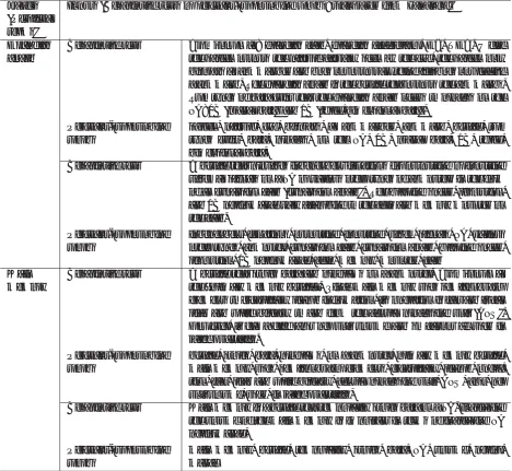
Labels (Retrieval terms)
Inputs (Descriptive texts or relevant/surrounding words; translated from Japanese)
Graphics board
Descriptive text Also known as: graphics card, graphics accelerator, GB, VGA. While the screen outputs the picture actually seen by the eye, the screen only displays as commanded and does not output anything if it does not receive a command. The graphics board is the device that outputs the commands. Two types of data exist that the graphics board needs to process on the PC: 2D (planar data) and 3D (three-dimensional data).
Relevant/surrounding words
screen, picture, eye, displays, as commanded, command, device, two types exist, data, process, on the PC, 2D, planar data, 3D, three-dimensional data.
Descriptive text A device that provides independent functions for outputting or inputting video as signals on a PC or various other types of computers in the form of an expansion card (expansion board). The drawing speed, resolution, and 3D performance vary according to the chip and memory mounted on the card.
Relevant/surrounding words
independent, functions, outputting, inputting, video, signals, PC, various other types, computer, expansion card, expansion board, drawing speed, resolution, 3D performance, chip, memory, mounted, card
Main memory
Descriptive text A device that stores data and programs on a computer. Also known as the ‘primary memory device’. Since main memory uses semiconductor elements to electrically record information, its operation is fast and it can read and write directly to and from the central processing unit (CPU). However, it has a high cost per unit volume and so cannot be used in large quantities.
Relevant/surrounding words
device, stores, data, programs, on a computer, primary memory device, main memory, uses, semiconductor elements, electrically, record, opera-tion, fast, read and write directly, central processing unit, CPU, cost, per unit volume, used, in large quantities.
Descriptive text Main memory is a device that temporarily stores data on a PC. Increasing the volume of the main memory is important in terms of increasing PC performance.
Relevant/surrounding words
main memory, device, temporarily, stores, data, PC, volume, perfor-mance
Table 1: Examples of input-label pairs in the corpus.
parts of phrasesͱ(toha, “what is”),(ha, “is”),
ͱ͍͏ͷ(toiumonoha, “something like”),ʹͭ ͍ͯ(nitsuiteha, “about”), and ͷҙຯ( noim-iha, “the meaning of”), on the labels to form the re-trieval terms (e.g., if a label is άϥϑΟοΫϘʔ υ (gurafikku boudo, “graphics board”), then the retrieval terms are άϥϑΟοΫϘʔυ ͱ ( gu-rafikku boudo toha, “what is graphics board”),άϥ ϑΟοΫϘʔυ (gurafikku boudo ha, “graphics board is”), etc.) and then use these terms to obtain the relevant Web pages by a Google search. Be-cause data gathered in this way might have incorrect labels, i.e., labels that do not match the descriptive
texts, we use them as unlabeled data. We obtained 25,000 pieces of data (i.e., inputs) in total.
2.3 Word Extraction and Feature Vector
Construction
Relevant/surrounding words are extracted from de-scriptive texts in steps (1)–(4) below, and the inputs are represented by feature vectors in machine learn-ing constructed in steps (1)–(6): (1) perform mor-phological analysis on the labeled data that are used for training and extract all nouns, including proper nouns, verbal nouns (nouns forming verbs by adding the word͢Δ(suru, “do”)), and general nouns; (2)
connect the nouns successively appearing as single words; (3) extract the words whose appearance fre-quency in each label is ranked in the top 30; (4) ex-clude the words appearing in the descriptive texts of more than 20 labels; (5) use the words obtained in the above steps as the vector elements with binary values, taking value 1 if a word appears and 0 if not; and (6) morphologically analyze all data described in Subsections 2.1 and 2.2, and construct the feature vectors in accordance with step (5).
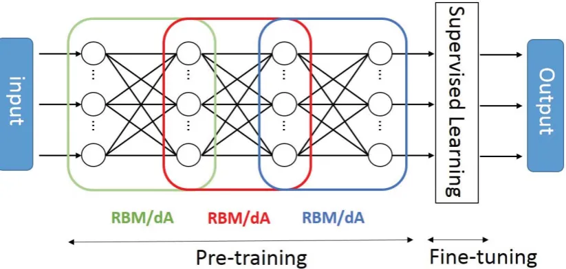
3 Deep Learning and Regularization Deep learning consists of unsupervised learning for pre-training to extract features and supervised learn-ing for fine-tunlearn-ing to output labels. Deep learnlearn-ing can be implemented by two typical approaches: us-ing deep belief networks (DBN) (Hinton et al., 2006; Lee et al., 2009; Bengio et al., 2007; Bengio, 2009; Bengio et al., 2013) and using stacked denoising autoencoders (SdA) (Bengio et al., 2007; Bengio, 2009; Bengio et al., 2013; Vincent et al., 2008; Vin-cent et al., 2010). The same supervised learning method can be used with both of these approaches; i.e., both approaches can be implemented with a single-layer or multi-layer perceptron or other tech-niques (linear regression, logistic regression, etc.), while a different unsupervised learning method is used; i.e., a DBN is formed by stacking restricted
Boltzmann machines (RBM), and an SdA is formed by stacking denoising autoencoders (dA) using a greedy layer-wise training algorithm. In this work, we use SdA as well as DBN, both of which use lo-gistic regression for supervised learning.
Figure 1 shows an example of deep neural net-works composed of three RBM or dA for pre-training and a supervised learning device for fine-tuning. Naturally the number of RBM/dA is change-able as needed. As shown in the figure, the hid-den layers of the earlier RBM/dA become the visible layers of the new RBM/dA.
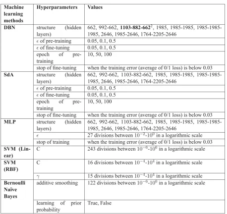
Machine learning methods
Hyperparameters Values
DBN structure (hidden
layers)
662, 992-662, 1103-882-6622, 1985, 1985-1985, 1985-1985-1985, 2646, 1985-2646, 1764-2205-2646
of pre-training 0.05, 0.1, 0.5
of fine-tuning 0.05, 0.1, 0.5 epoch of
pre-training
10, 50, 100
stop of fine-tuning when the training error (average of 0/1 loss) is below 0.03
SdA structure (hidden
layers)
662, 992-662, 1103-882-662, 1985, 1985-1985, 1985-1985-1985, 2646, 1985-2646, 1764-2205-2646
of pre-training 0.05, 0.1, 0.5
of fine-tuning 0.05, 0.1, 0.5 epoch of
pre-training
10, 50, 100
stop of fine-tuning when the training error (average of 0/1 loss) is below 0.03
MLP structure (hidden
layers)
662, 992-662, 1103-882-662, 1985, 1985-1985, 1985-1985-1985, 2646, 1985-2646, 1764-2205-2646
27 divisions between10−2-100 in a logarithmic scale stop of training when the training error (average of 0/1 loss) is below 0.03
SVM (Lin-ear)
C 243 divisions between10−6-106 in a logarithmic scale
SVM (RBF)
C 16 divisions between10−4-104 in a logarithmic scale
γ 15 divisions between10−4-104 in a logarithmic scale
Bernoulli Na¨ıve Bayes
additive smoothing 122 divisions between10−6-100 in a logarithmic scale
learning of prior probability
True, False
Table 2: Hyperparameters for grid search used in the comparative experiments of different training data sets and different machine learning methods without regularization.
weights are multiplied by 1-p.
2As an example, the structure (hidden layers)1103-882-662, shown as bold in the table, refers to a DBN with a 1323-1103-882-662-100 structure, where 1323 and 100 respectively refer to dimensions of the input and output layers. These figures were set not in an arbitrary manner. The first three structures are de-creasing (pyramid-like) size and all hidden layers were set to 3/6, 4/6, 3/4, and 5/6 times smaller than that of the input layer, i.e.,662 = 1323×3/6,882 = 1323×4/6,992 = 1323×3/4, and 1103 = 1323×5/6. The last three structures are in-creasing (upside down pyramid) size and all hidden layers were set to 8/6, 9/6, 10/6, and 12/6 times larger than that of the in-put layer, i.e., 1764 = 1323×8/6, 1985 = 1323×9/6, 2205 = 1323×10/6, and2646 = 1323×12/6. The middle
4 Experiments
4.1 Experimental Setup
We used three data sets with different amounts of data (i.e., 1,134 labeled data; 1,134 labeled data + 13,000 unlabeled data; and 1,134 labeled data + 25,000 unlabeled data) for unsupervised learning, the same 1,134 labeled data for supervised learning, and the remaining 100 labeled data for testing. The
three structures were set in accordance with the recommenda-tions of (Bengio, 2012) that using the same size works gener-ally as well as or better than using a decreasing (pyramid-like) or increasing (upside down pyramid) size.
N=1 N=5 N=10
BNB 0.773 0.772 0.770
MLP 0.780 0.789 0.790
SVM (Linear) 0.807 0.807 0.804
SVM (RBF) 0.717 0.719 0.716
DBN 0.793 0.811 0.808
SdA 0.810 0.817 0.818
Table 3: Average precisions values obtained using different methods without regularization.
1 5 10 15 20 25 30 Top N
0.77 0.78 0.79 0.80 0.81 0.82 0.83
Average pr
ecision
No regularization L1 regularization L2 regularization Dropout
MLP
1 5 10 15 20 25 30 Top N
0.77 0.78 0.79 0.80 0.81 0.82 0.83
Average pr
ecision
No regularization L1 regularization L2 regularization Dropout
DBN
1 5 10 15 20 25 30 Top N
0.77 0.78 0.79 0.80 0.81 0.82 0.83
Average pr
ecision
No regularization L1 regularization L2 regularization Dropout
SdA
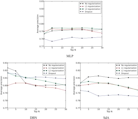
Figure 4: Comparison of average precision values obtained with and without regularization.
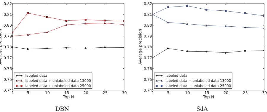
when using the top N sets of the hyperparameters in ascending order of the cross-validation errors, with N varying from 1 to 30. As shown in the figure, the precision of both DBN and SdA can be improved by adding the unlabeled data to the labeled data as training data, and both DBN and SdA have higher
precision when using a larger amount of unlabeled data.
Figure 3 compares the testing data precision val-ues obtained when using the largest data set (1,134 labeled data + 25,000 unlabeled data) for unsuper-vised learning, when using different learning
BNB 0.773 0.773 0.773
MLP 0.787 0.791 0.791
MLP with L1 0.790 0.793 0.792
MLP with L2 0.787 0.795 0.794
MLP with Dropout 0.780 0.777 0.780
SVM (Linear) 0.807 0.809 0.807
SVM (RBF) 0.730 0.737 0.735
DBN 0.823 0.819 0.803
DBN with L1 0.800 0.803 0.803
DBN with L2 0.817 0.813 0.811
DBN with Dropout 0.817 0.815 0.810
SdA 0.803 0.811 0.813
SdA with L1 0.800 0.801 0.803
SdA with L2 0.803 0.805 0.803
SdA with Dropout 0.793 0.792 0.789
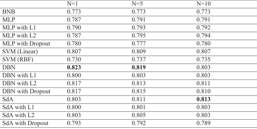
Table 4: Average precision values obtained using different methods with and without regularization.
ods and Bernoulli Na¨ıve Bayes (BNB), which is used as a baseline. We can see at a glance from the figure that the performance of SdA is superior to that of DBN and that both DBN and SdA are generally superior to BNB, MLP, and SVM. We should point out that the results for SVM (RBF) are not indicated in the figure because the precision values were lower than 0.74. Table 3 lists the specific average preci-sion values obtained using different learning meth-ods when N=1, 5, and 10.
Figure 4 and Table 4 compare the testing data precision values for MLP, DBN, and SdA with and without regularization3. The figure and table show that the performance of MLP and DBN improved in some cases by using regularization, whereas no per-formance improvement can be found for SdA. How-ever, both DBN and SdA outperformed BNB, MLP and SVM whether regularization was used or not.
5 Conclusion
We presented methods to predict retrieval terms from relevant/surrounding words or descriptive texts in Japanese by using deep belief networks (DBN)
3
It should be noted that the precision values obtained with-out regularization (shown in Figure 4 and Table 4) differ from those shown in Figure 3 and Table 3. This is because different numbers of hyperparameter sets were used for grid searching between the two experiments as described in Subsection 4.1.
and stacked denoising autoencoders (SdA). Experi-mental results based on a relatively large scale con-firmed that (1) adding automatically gathered unla-beled data to the launla-beled data for unsupervised learn-ing was an effective measure for improvlearn-ing the pre-diction precision, and (2) using either DBN or SdA definitely achieved higher prediction precision than that obtained using multi-layer perceptron (MLP), whether weight decay (L2 regularization), sparsity (L1 regularization), or dropout regularization was used. Both DBN and SdA achieved higher preci-sion than Bernoulli Na¨ıve Bayes (BNB) and support vector machines (SVM).
In the future, we plan to start developing var-ious practical domain-specific systems that can predict suitable retrieval terms from the rele-vant/surrounding words or descriptive texts.
Acknowledgments
This work was supported by JSPS KAKENHI Grant Number 25330368.
References
M. Auli, M. Galley, C. Quirk, and G. Zweig. 2013. Joint Language and Translation Modeling with Recurrent Neural Networks. EMNLP 2013, 1044–1054.