ABSTRACT
RUBLE, MACEY CHARLES. Massive MIMO Millimeter Wave Channel Estimation and Localization. (Under the direction of Dr. ˙Ismail Güvenç).
Fifth generation (5G) cellular standards are set to utilize millimeter wave (mmWave) frequencies
above 24 GHz. The small wavelength associated with mmWave frequencies allow massive
multiple-input-multiple-output (MIMO) antenna arrays to fit in small spaces, which contain hundreds or
thousands of antenna elements at the transmitter and receiver. Massive MIMO arrays and
ultra-wide bandwidths of mmWave signals enable communication rates and localization performance
orders of magnitude better than previous cellular systems. However, a number of signal processing
challenges must be addressed for these capabilities to be achieved. This dissertation addresses the
signal processing challenges of mmWave technology, specifically focusing on channel estimation
and localization.
Channel estimation for massive MIMO systems is a challenge because of the large amount of
data streaming from the antenna arrays. Orthogonal frequency division multiplexing (OFDM) adds
further complications since the channel must be estimated at each subcarrier, making channel
estimation a high-dimensional estimation problem. Channel estimation at mmWave frequencies
relies on accurate estimates of the channel parameters, which we define as the angle of arrival,
angle of departure, and path distance for each path between the transmitter and receiver. This
dissertation introduces a channel parameter estimation technique based on the multilinear singular
value decomposition (MSVD), a tensor analogue of the singular value decomposition, for massive
MIMO multi-carrier systems with hybrid analog/digital beamforming. The MSVD tensor estimation
approach provides a computationally efficient channel parameter estimation method and is shown
to closely match the Cramer-Rao bound (CRB) through simulations. Additionally, the dictionary
resolution required to detect the optimal channel parameter estimates is derived.
A significant advantage of mmWave systems is that non-line of sight (NLOS) paths can be
as the reflector locations for NLOS paths must also be estimated for a reliable receiver location
estimate. This results in a high-dimensional non-convex estimation problem. It will be shown in
this dissertation that channel parameter estimates from multiple paths are sufficient to estimate the
receiver location as well as the reflection locations for the NLOS paths. A gradient-assisted particle
filter (GAPF) estimator is proposed, which uses the channel parameters to accurately estimate a
receiver location as well as the locations of nearby scatterers. The GAPF is developed to be used in
scenarios with one or multiple transmitting nodes and utilize both line-of-sight (LOS) and NLOS link.
The GAPF estimator is applied to localization in urban environments and networks with/without
radio-environmental mapping (REM) are considered, where a network with REM is able to localize
nearby scatterers. Monte Carlo simulations show that the GAPF estimator performance matches
the Cramer-Rao bound (CRB). The estimator is also used to create an REM. It is seen that significant
localization gains can be achieved by increasing beam directionality or by utilizing REM.
Estimating the reflector location nuisance parameters for all of the NLOS paths adds
com-plexity to localization. However, environmental maps can supplement localization by providing
estimates for the reflector locations, or map-based reflector location estimates (MRLE). This
dis-sertation introduces the map-based localization bound (MLB) as a bound for receiver localization
performance when MRLE is used to estimate reflector locations for NLOS paths. Results show that
receiver localization utilizing MRLE only offers improvement if MRLE errors can be reduced below
© Copyright 2018 by Macey Charles Ruble
Massive MIMO Millimeter Wave Channel Estimation and Localization
by
Macey Charles Ruble
A dissertation submitted to the Graduate Faculty of North Carolina State University
in partial fulfillment of the requirements for the Degree of
Doctor of Philosophy
Electrical Engineering
Raleigh, North Carolina
2018
APPROVED BY:
Dr. Hans Hallen Dr. Edgar Lobaton
Dr. Mihail Sichitiu Dr. Alexandra Duel-Hallen
DEDICATION
BIOGRAPHY
The author attended the University of North Carolina at Charlotte and graduated with degrees in
Physics and Mathematics. The author began graduate school with a MS in Applied Physics from
Cornell University. Then, the author changed fields to Electrical and Computer Engineering to
ACKNOWLEDGEMENTS
I would like to thank my advisor, Dr. Guvenc for his help and the other members of the group for
their insightful comments. Additionally, I would like to thank my committee members for their
positive feedback and assistance. The work in this dissertation has been supported in part by the
TABLE OF CONTENTS
LIST OF TABLES . . . .viii
LIST OF FIGURES. . . ix
Chapter 1 INTRODUCTION . . . 1
1.1 Abbreviations . . . 1
1.2 Motivation . . . 2
1.3 Literature Review . . . 4
1.3.1 Channel Estimation . . . 4
1.3.2 Localization . . . 5
1.4 Layout and Contributions . . . 8
1.4.1 Chapter 2 . . . 8
1.4.2 Chapter 3 . . . 8
1.4.3 Chapter 4 . . . 9
1.4.4 Chapter 5 . . . 9
1.4.5 Chapter 6 . . . 10
Chapter 2 Channel Parameter Estimation. . . 11
2.1 Introduction . . . 11
2.1.1 Relevant Literature . . . 12
2.1.2 Contributions . . . 13
2.1.3 Chapter Organization . . . 14
2.2 Broadband MIMO OFDM Model . . . 15
2.2.1 MIMO OFDM Channel Model . . . 15
2.2.2 Tucker Tensor Form . . . 17
2.2.3 The Channel in Tucker Tensor Form . . . 18
2.3 Problem Formulation for mmWave Channel Parameter Estimation . . . 21
2.4 Multilinear SVD for mmWave Channel Parameter Estimation . . . 22
2.4.1 The Multilinear Singular Value Decomposition . . . 22
2.4.2 Rank Reduction . . . 23
2.4.3 Separating Channel Parameter Estimation into Separate Subspace Problems 24 2.4.4 Subspace Estimation . . . 26
2.4.5 Super-Resolution Channel Parameter Estimation . . . 28
2.4.6 MSVD Basis Transformation . . . 28
2.4.7 Linking Channel Parameters to Paths . . . 29
2.4.8 Estimating Path Gain . . . 31
2.4.9 Applications of Channel Parameter Estimation . . . 32
2.5 Waveform Considerations for MIMO OFDM Channel Parameter Estimation . . . 32
2.5.1 Frequency Selectivity . . . 32
2.5.2 Effective SNR . . . 33
2.5.3 Distance Redundancy . . . 33
2.6.1 SNR and Numbers of Antenna Elements . . . 36
2.6.2 Training Symbol Length . . . 37
2.6.3 Number of Subcarriers . . . 39
2.7 Conclusion . . . 40
Chapter 3 Channel Parameter Estimation Resolution . . . 43
3.1 Introduction . . . 43
3.2 General Measurement Model and Problem Formulation . . . 44
3.3 Channel Parameter Resolution . . . 45
3.4 AOA Subspace . . . 45
3.4.1 AOD Subspace . . . 47
3.4.2 Path Distance . . . 47
3.5 Viewing the Channel Parameterl2Curves . . . 49
3.6 Conclusion . . . 51
Chapter 4 Localization in Urban Environments . . . 52
4.1 Introduction . . . 52
4.1.1 Contributions of This Chapter . . . 54
4.2 mmWave Localization System Model . . . 55
4.2.1 Localization Model . . . 56
4.2.2 Statistics of AOA, AOD, and TOA . . . 61
4.2.3 Differentiating LOS and NLOS Paths . . . 62
4.3 mmWave Location Estimation . . . 64
4.3.1 Maximizing the Likelihood Function . . . 64
4.3.2 Non-REM Assisted Localization . . . 65
4.3.3 REM Assisted Localization . . . 66
4.3.4 Gradient Methods . . . 66
4.3.5 Particle Filters . . . 67
4.3.6 Gradient-Assisted Particle Filter . . . 68
4.3.7 Initialization . . . 69
4.4 Fundamental Lower Bounds for mmWave Localization . . . 71
4.5 Numerical Results and Discussion . . . 74
4.5.1 Localization Performance as a Function of Beamwidth . . . 75
4.5.2 Localization in Urban Environments . . . 77
4.5.3 Building REM from Localization Outcomes . . . 81
4.6 Conclusion . . . 83
Chapter 5 Bounds for Map-Based Millimeter Wave Localization . . . 85
5.1 Introduction . . . 85
5.2 Localization System Model . . . 86
5.3 Bounding Localization with MRLE . . . 89
5.3.1 Reflector Dilution of Precision . . . 90
5.4 Numerical Results . . . 91
5.4.2 RDOP as a Function of Path Reflector Angle . . . 93
5.4.3 RDOP as a Function of Distance . . . 95
5.5 Conclusion . . . 95
Chapter 6 Conclusion. . . 96
6.1 Concluding Remarks . . . 96
6.2 Publications . . . 98
BIBLIOGRAPHY . . . 99
APPENDICES . . . .104
Appendix A CRB Derivation for Channel Parameter Estimation . . . 105
LIST OF TABLES
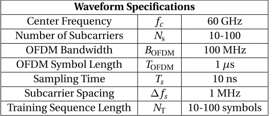
Table 2.1 Range of waveform specifications considered in simulations. . . 34
LIST OF FIGURES
Figure 2.1 MIMO OFDM channel model with hybrid beamforming. . . 13
Figure 2.2 Channel parameters for a path between the transmitter array and receiver array. . . 18
Figure 2.3 Vector-wise outer product view of Tucker model. . . 20
Figure 2.4 Full Tucker tensor form. . . 21
Figure 2.5 The measurement tensorY is sizeLrx×NT×NswhereLrxis the number of data streams,NTis the number of training symbols, andNsis the number of subcarriers. The reduced rank Tucker form from the MSVD selects the strongest components from each subspace. . . 24
Figure 2.6 A basis transformation converts from an orthogonal MSVD basis to a non-orthogonal dictionary basis. . . 25
Figure 2.7 Overdetermined problem to compute the column subspace basis transfor-mationQ1. . . 25
Figure 2.8 Linking channel parameters for each path. . . 30
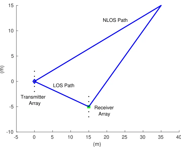
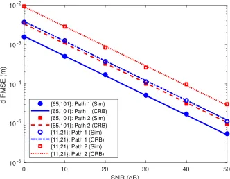
Figure 2.9 Path geometry for channel parameter simulations. . . 36
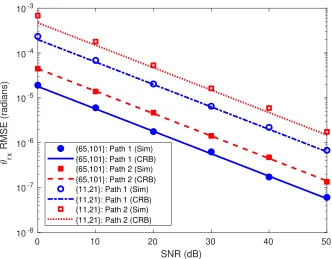
Figure 2.10 Simulatedθrx,nestimation RMSE and CRB for the paths in Fig. 2.9 withNr x= 11,Nt x=21 andNr x=65,Nt x =101 for both pathsn=1, 2. . . 37
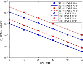
Figure 2.11 Simulatedθtx,nestimation RMSE and CRB for the paths in Fig. 2.9 withNr x= 11,Nt x=21 andNr x=65,Nt x =101 for both pathsn=1, 2. . . 38
Figure 2.12 Simulateddnestimation RMSE and CRB for the paths in Fig. 2.9 withNr x= 11,Nt x=21 andNr x=65,Nt x =101 for both pathsn=1, 2. . . 39
Figure 2.13 Simulatedhn estimation RMSE and CRB for the paths in Fig. 2.9 withNr x= 11,Nt x=21 andNr x=65,Nt x =101 for both pathsn=1, 2. . . 40
Figure 2.14 Path 1 channel parameters as a function of training symbol length (NT) at SNR=5 dB. . . 41
Figure 2.15 Path 1 channel parameters as a function of the number of subcarriers (Ns) at SNR=5 dB. . . 42
Figure 3.1 AOAl2curve. . . 49
Figure 3.2 Path distancel2curve. . . 50
Figure 4.1 Signal propagation in microwave and mmWave frequencies. . . 53
Figure 4.2 mmWave localization model for (a) NLOS and (b) LOS scenarios. . . 57
Figure 4.3 (a) Geometry and ray tracing paths for Wireless Insite simulation in an urban environment. Paths are colored based on RSS where the strongest RSS path is red and the weakest RSS paths is green. (b) TOA of simulation with 80◦3 dB beamwidth. (c) TOA of simulation with 28◦3 dB beamwidth. . . 63
Figure 4.4 One iteration of the GAPF estimator. . . 70
Figure 4.6 (a) Urban canyon with one FE, one LOS path, and one NLOS path. (b) CDF of RMSE. (c) RMSE at 73 GHz without REM. (d) RMSE at 73 GHz with REM. (e) Improvement in RMSE with REM at 73 GHz. . . 78 Figure 4.7 (a) Urban canyon with two FEs, two LOS paths, and two NLOS paths. (b) CDF
of RMSE. (c) RMSE at 73 GHz without REM. (d) RMSE at 73 GHz with REM. (e) Improvement in RMSE with REM at 73 GHz. . . 79 Figure 4.8 (a) Urban corner with one FE, one LOS path, and two NLOS paths. (b) CDF of
RMSE. (c) RMSE at 73 GHz without REM. (d) RMSE at 73 GHz with REM. (e) Improvement in RMSE with REM at 73 GHz. . . 81 Figure 4.9 (a) Urban corner with two FEs, two LOS paths, and two NLOS paths. (b) CDF
of RMSE. (c) RMSE at 73 GHz without REM. (d) RMSE at 73 GHz with REM. (e) Improvement in RMSE with REM at 73 GHz. . . 82 Figure 4.10 Mapped scatterer locations (red) generated from GAPF estimator at UE
lo-cations (green) on a path through (a) the urban canyon and (b) the urban corner. . . 83
Figure 5.1 Illustration of the UE location estimation error that results from errors in map-based reflector location estimates. . . 87 Figure 5.2 (a) One LOS path and one NLOS between a FE and a UE. (b) Simulated
local-ization with MRLE and theoretical MLB versus reflector location estimation error using the paths from (a). The CRB for localization without MRLE is also shown. . . 92 Figure 5.3 (a) A NLOS path with fixed FE to reflector distanced1=20 (m) and a fixed
reflector to UE distanced2=30 (m). The path reflection angleφis varied. (b) MLB and RDOP as a function of path reflection angleφ. . . 93 Figure 5.4 (a) A NLOS path travels distanced1=20 (m) from the FE to the reflector
CHAPTER
1
INTRODUCTION
1.1
Abbreviations
mmWave: Millimeter Wave
MIMO: Multiple Input Multiple Output
MSVD: Multilinear Singular Value Decomposition
OFDM: Orthogonal Frequency Division Multiplexing
ADC: Analog to Digital Converter
OMP: Orthogonal Matching Pursuit
GPS: Global positioning system
LOS: Line-of-sight
TOA: Time-of-arrival
AOD: Angle-of-departure
AOA: Angle-of-arrival
TDOA: time-difference-of-arrival
UE: User equipment
FE: Fixed equipment
GAPF: Gradient-assisted particle filter
REM: Radio-environmental mapping
ML: Maximum likelihood
CRB: Cramer-Rao bound
MSE: Mean square error
RMSE: Root-mean square error
CDF: Cumulative distribution function
MRLE: Map-based Reflection Location Estimate
MLB: Map-based Localization Bound
1.2
Motivation
The demand for wireless broadband communication has been growing rapidly, which has been the
driving force for the emergence of 5G cellular networks. 5G networks are set to deploy millimeter
wave (mmWave) technology, which employs carrier frequencies from 30−300 GHz[Zhup ; Rapy ; Rapp ; Macne]. Unique properties of mmWave frequencies enable mmWave technology to reach
data rates over 10 Gigabits per second (Gbps)[Rapy]and receiver localization accuracy less than
1 cm[Sha18]. The high performance communication capacity and localization with mmWave
technology will enable a new era of large data cell phone applications, user tracking, and augmented
potential. The focus of this dissertation is on offering solutions to the signal processing challenges
associated with mmWave technology. In particular, this dissertation studies mmWave channel
estimation and localization. Prior to introducing these problems, the unique properties of mmWave
technology that enable high performance communication and localization are layed out since they
play an important role in formulating the problems in this dissertation. The unique properties of
mmWave technology are:
• The small wavelength of mmWave frequencies allows massive multiple-input-multiple-output
(MIMO) arrays to be deployed in small spaces[Zhup], which have hundreds to thousands of
antenna elements at the transmitter and receiver.
• Large attenuation is observed during reflection at mmWave frequencies, which allows a single
bounce assumption for non-line of sight (NLOS) paths, where each NLOS path is assumed to
have only reflected off of a single surface[DSne; Rapn].
• Highly directional beams and large path attenuation result in very few paths that have
sig-nificant received signal strength. This leads to a sparse propagation channel, which can be
completely represented by characterizing the few significant paths[DSne; Sha18]. Channel
sparseness is a key element in signal processing for mmWave technology as the reduced
number of parameters enable a path model based representation of the channel. Contrary to
this, lower frequencies are unable to separate paths because of rich and complex multipath,
which obliges the channel to be represented as a random quantity.
• MmWave frequencies allow the use of ultra-wide bandwidths larger than 1 GHz. This gives
better communication performance and helps in providing precise time of arrival (TOA)
estimates[Zhup].
• Unlike lower frequencies, where NLOS paths are treated as interference, NLOS paths can be
exploited at mmWave frequencies as paths that contain useful information[Menc].
frequencies. Channel estimation is accomplished by transmitting a known training sequence so that
the environmental impacts on the channel can be determined and accounted for when unknown
data sequences are transmitted. 5G networks will use orthogonal frequency division multiplexing
(OFDM) or OFDM-like waveforms, which enable broadband communication by distributing the
transmitted data over many subcarrier frequencies[Sha18; Gua17; SY17; Ham13]. Therefore, the
channel must be estimated at each subcarrier frequency. An antenna with an analog to digital
converter (ADC) at every single antenna element becomes too costly for large arrays. Thus, a
channel estimation method must function with hybrid digital/analog beamforming, which uses
digital beamforming as well as phased array analog beamforming to reduce the overall number of
required ADCs[SY17; Alk14]. The sparsity of the mmWave channel reduces the channel estimation
problem for all OFDM subcarriers to estimating the angle of arrival (AOA), angle of departure (AOD),
and total transmitter to receiver path distance for each of the significant paths[Sha18; SY17; Alk14].
We define the AOA, AOD, and path distance parameters for all of the significant paths as the channel
parameters.
A second focus of this dissertation is localization, which also relies on estimating the channel
parameters. The predominant challenge for localization at mmWave frequencies is utilizing NLOS
paths. This leads to a high-dimensional non-convex estimation problem. The benefit of utilizing
NLOS paths for localization is estimated reflector locations for the NLOS paths, which can be used
to build an environmental map.
1.3
Literature Review
1.3.1 Channel Estimation
Massive MIMO channel estimation has received much recent attention in the literature[DSne; Sha18;
SY17; Alk14; Rapp ; Andn ; Zha18; Sur16; BS15]. However, a number of problems have yet to be solved.
Much work has focused on two-dimensional coordinate system channel parameter estimation
channel parameter estimation and localization in two dimensions, but this method doesn’t scale to
scenarios when both the azimuthal and elevation angles must be considered. While[AS17]derives
bounds for three-dimensional channel parameter estimation, an efficient estimation method that
can handle higher dimensional scenarios is still of remaining interest. Channel estimation with
elevation and azimuthal angles become much more difficult because of the extra dimensionality
of the problem. Especially considering the number of significant paths is unknown and must be
estimated. Localization is inherently linked to channel parameter estimation since the channel
parameters for mutliple paths are sufficient information for receiver tracking and environmental
mapping[DSne; Sha18; RGn].
Many applications are arising that require high dimensional parameter estimation, which can
be grouped into tensor form[Hay17],[NS10],[Sid17]. Efficient methods have been developed for
estimation with tensors[Sid17]. Of particular importance is the multilinear singular value
decom-position (MSVD), which is a tensor analogue of the singular value decomdecom-position commonly seen
in linear algebra. The MSVD allows efficient estimation of parameters from low rank tensors. It
is known that MIMO OFDM receiver measurements can be grouped into low rank tensor forms
[Zho17], which provides opportunities for tensor channel estimation approaches.
1.3.2 Localization
Receiver localization is of particular interest because it can improve other features of a mmWave
system. It has been shown that the knowledge acquired from receiver localization can be used to
reduce the time spent on initial acces and increase capacity[Sal17],[Masc], where initial access or
beamsearch is the process required to aim the highly directional transmit and receive beams to
obtain a desired SNR. Additionally, knowledge of the receiver location and reflection locations for
all paths greatly simplifies channel parameter estimation[DSne].
There have been recent studies in the literature that evaluate mmWave localization performance
in various scenarios. Localization with received signal strength (RSS), TOA, and AOA are analyzed in
showing promising results with TOA and AOA, and less reliable results with RSS. A log-normal
path loss model is used to evaluate RSS, time-difference-of-arrival (TDOA), and AOA localization
methods for LOS paths in[ESc]. Wireless localization with strictly NLOS paths is achievable for
omni-directional antennas by exploiting the time-of-arrival (TOA), of-arrival (AOA) and
angle-of-departure (AOD) measurements[GC09; Mia07; Hanc]. A mobile’s location and orientation
are estimated jointly in[Guene; Shac]for mmWave systems. It is shown in these papers that a
single fixed equipment (FE) is sufficient to localize a user equipment (UE), but only LOS paths
are considered. Also of interest is[Hanc], which derives the Cramer-Rao bound for wideband
localization and arbitrary antenna size for moving user. It is shown that the Doppler shift caused
by the moving user contributes to localization accuracy. The work in[Gar17]introduces a direct
localization approach for a user connected with multiple transmitters that separates LOS from
NLOS paths and uses fine estimation of AOA and coarse estimation of TOA to directly estimates
a user’s position. NLOS paths are treated as interference, and thus, this method only utilizes LOS
paths.
The previously mentioned works do not use the information carried by NLOS paths. However,
NLOS paths can be exploited for localization with or without LOS paths. For mmWave technology,
non-line of sight (NLOS) paths are not treated as interference, but rather as additional paths that
carry useful information[Menc]. This enables the reflection locations to be estimated making
simultaneous localization and mapping (SLAM) possible, where the receiver is localized while the
environment is mapped in parallel[Witr ; RGn]. The authors in[Menc]use the concept of Fisher
information to show that NLOS paths carry additional information, which can be used to improved
localization accuracy. It is shown in[DSne]that the mmWave signals have a sparse beamspace,
which leads to a simple channel that can be separated into distinct paths allows localization without
a LOS path.
The work in[Sha18]shows that is is possible to determine the orientation and position of a user
communicating with a single transmitter at mmWave frequencies using NLOS paths under certain
shown that sufficient conditions for position and orientation estimation require at least one LOS
path or three NLOS paths. The Cramer-Rao bound for localization and orientation is derived and a
localization algorithm is proposed.The authors first estimate AOD/AOA/TOA, which is done in three
stages. The first stage exploits the sparsity of the mmWave channel in the angular domain to estimate
AOD and AOA. The second stage uses the AOD and AOA estimates to estimate TOA. The third stage
uses a maximum likelihood approach to refine the grid. Following this, the AOD/AOA/TOA estimates
are used to estimate the position and orientation of the receivers. However, it should be noted
that only the single transmitter case is considered and scenarios may exist where more than one
transmitter must be used to locate a receiver. The authors in[Sha18]consider two dimensions, but
[AS17]extends the position error and orientation error Cramer-Rao bound calculations to three
dimensions and a uniform rectangular array antenna.
Similar to the channel estimation literature, much work has focused on two-dimensional
lo-calization, but these methods don’t scale to three dimensional scenarios when both the azimuthal
and elevation angles must be considered. While[AS17]derives bounds for three dimensional
lo-calization, an efficient estimation method that can handle higher dimensional scenarios is still of
remaining interest. Furthermore, estimating the TOA, AOA, and other related parameters is only the
first step. A difficult second step is grouping the parameters to particular paths. The[Sha18]needs
to be extended so that all of the subcarriers can be utilized simultaneously for each estimate. While
it is possible to locate a receiver with resolution less than a centimeter, it is a challenge to process
the high-dimensional data that streams from the massive MIMO arrays[Sha18]. Receiver location
tracking and environmental mapping requires estimation over a high-dimensional non-convex
space with many local optima[RGn].
Another area of interest is in radio-environmental mapping (REM), which maps the three
dimen-sional structure of the environment so that it can later be exploited to estimate scatterer locations for
NLOS paths to improve localization[LB16]. The knowledge provided by localization and REM can
be used to relax initial access requirements and improve capacity for 5G communication systems
using LOS and NLOS paths. Tracking algorithms are considered and simultaneous localization and
mapping (SLAM) is used as a means to build an environmental map, which can later be exploited to
improve user tracking. Then, the idea of cognitive localization and tracking is introduced, which
jointly updates and shares information during localization and environmental mapping. This
im-proves system performance as localization with SLAM provides information that can be used to map
the environment. Additionally, the information provided by mapping can reduce the localization
search space and can be used to improve location estimates during user tracking. Similarly, the work
in[LB16]provides an algorithm that uses a mapping of the 3D environment to improve localization
accuracy.
1.4
Layout and Contributions
1.4.1 Chapter 2
Chapter 2 addresses the processing of the high-dimensional data streams from OFDM massive
MIMO systems to estimate the channel parameters. Many existing solutions only focus on azimuthal
angle and do not scale to include elevation angle. This chapter introduces a channel parameter
estimation algorithm that groups receiver measurements into tensors and utilizes the MSVD for
estimation. The advantage to this method is that it scales to higher dimensional tensors and still
provides computationally efficient estimation. Additionally, the proposed method estimates the
number of significant paths as well as links the channel parameters to particular paths. Simulations
show that the proposed technique closely matches the CRB. Limitations of channel parameter
estimation and communication waveform effects are also studied.
1.4.2 Chapter 3
The algorithm in Chapter 2 relies on a dictionary of channel parameter values. Too many dictionary
terms slow down the algorithm, but too few dictionary terms may not have enough coverage to
peaks under thel2optimality criterion. This provides the dictionary grid spacing that is required to
detect the optimal channel estimates.
1.4.3 Chapter 4
The algorithm proposed in[Sha18]performs localization at mmWave frequencies using LOS and
NLOS paths. However, it is only suited for single FE scenarios. There may be scenarios where a single
transmitter is unable to establish enough paths to meet the sufficient conditions for localization.
Alternatively,[Gar17]implements a localization approach that can use paths from multiple FE, but
NLOS paths are treated as interference and only LOS paths are used for localization purposed.
Chapter 4 introduces a localization approach that utilizes the channel parameters from LOS and
NLOS paths from a single or multiple FE, which are obtained during beam alignment[Sha18],[Gio16].
Rather than using the super-resolution channel parameter estimates from the algorithm in Chapter
2, a reduced complexity approach is employed to obtain rough channel parameter estimates. A
gradient-assisted particle filter (GAPF) estimator is proposed as a maximum likelihood (ML)
esti-mator to estimate the receiver position and scatterer coordinates over a non-convex space. It is
shown to have performance that matches the Cramer-Rao bound (CRB) through Monte-Carlo
simu-lations. Localization performance is analyzed in urban canyon and urban corner scenarios where a
receiver is connected with one or two transmitters. The localization accuracy of REM-assisted and
non-REM-assisted network performance is analyzed. Furthermore, the scatterer locations that are
extracted from the proposed localization approach are used to create an REM.
1.4.4 Chapter 5
Typically, NLOS paths require estimation of one or more reflector locations for the NLOS path(s),
considered as nuisance parameters during the localization process. However, environmental maps
can supplement localization by providing estimates for the reflector locations, or map-based
reflec-tor location estimates (MRLE). In Chapter 5, the map-based localization bound (MLB) is introduced
for NLOS paths. Results show that receiver localization utilizing MRLE only offers improvement if
MRLE errors can be reduced below a threshold.
1.4.5 Chapter 6
Chapter 6 provides concluding remarks and discusses how the work in this dissertation can be
CHAPTER
2
CHANNEL PARAMETER ESTIMATION
2.1
Introduction
High performance communication and localization for mmWave technology are both dependent
on accurate estimates of the channel parameters, which we define as the angle of arrival (AOA),
angle of departure (AOD), and total transmitter to receiver path distance for each significant path.
This dependence is a result of highly directional beams and large path reflection attenuation, which
leads to few significant received paths and a sparse channel that is completely characterized by the
channel parameters[DSne]. Channel estimation for mmWave is accomplished by transmitting a
known training sequence so that the environmental impacts on the channel can be determined and
accounted for when unknown data sequences are transmitted[Sha18; SY17; Alk14]. The channel
parameters from multiple paths can also be simultaneously utilized to estimate a receiver’s position
5G networks will use orthogonal frequency division multiplexing (OFDM) or OFDM-like
wave-forms, which enable broadband communication by distributing the transmitted data over many
subcarrier frequencies[Sha18; Gua17; SY17; Ham13]. Channel parameter estimation is particularly
challenging for MIMO OFDM systems since the channel is different at each subcarrier. An antenna
with an analog to digital converter (ADC) at every single antenna element becomes too costly for
large arrays. Thus, a channel parameter estimation method must function with hybrid digital/analog
beamforming, which uses digital beamforming as well as phased array analog beamforming to
reduce the overall number of required ADCs[SY17; Alk14]. Adding to the challenge is that the
number of significant received paths is unknown and needs to first be estimated. Furthermore, a
collection of AOA, AOD, and path distance estimates is not a complete solution: a complete solution
must also link each estimated channel parameter to particular paths.
2.1.1 Relevant Literature
Massive MIMO channel parameter estimation has received much recent attention in the literature
[DSne; Sha18; SY17; Alk14; Rapp ; Andn ; Zha18; Sur16; BS15], but it still remains a challenge to utilize
all of the subcarriers simultaneously for OFDM systems and process the high-dimensional data that
streams from the massive MIMO arrays. These works focus on channel parameter estimation where
the transmitter and receiver are all on the same plane. However, these methods may not scale to
higher dimensional scenarios when both the azimuthal and elevation angles for AOD and AOA must
be considered.
High accuracy mmWave localization enables a new era of user tracking and augmented reality
[DSne; Shac ; Garr ; Gar17; Witr]. The work in[Sha18]estimates channel parameters and shows that
the channel parameters for a few paths are sufficient to estimate a receiver’s position and orientation.
Additionally, mmWave non-line of sight (NLOS) paths are not treated as interference, but rather as
additional paths that carry useful information[Menc ; DSne]. This enables the reflection locations to
be estimated from the channel parameters; making simultaneous localization and mapping (SLAM)
IFFT IFFT IFFT RF Chain Digital
Precoder RF Chain
RF Chain Analog Precoder Channel Analog Combiner RF Chain RF Chain RF Chain FFT FFT FFT Digital Combiner
Figure 2.1MIMO OFDM channel model with hybrid beamforming.
Many other applications are arising that require high dimensional parameter estimation. It has
been shown that these problems can be solved efficiently in tensor form[Hay17; NS10; Sid17; Ten].
Of particular importance is the multilinear singular value decomposition (MSVD), which is a tensor
analogue of the singular value decomposition (SVD) commonly seen in linear algebra. The MSVD
allows computationally efficient parameter estimation if the tensor is low rank and is often used in
machine learning[Sid17; Ten].
MSVD tensor estimation techniques are ideal for channel parameter estimation since an OFDM
MIMO receiver measurement can be represented in a low rank tensor form as shown in[Zho17].
This is achieved by grouping the receiver measurements into a low rank canonical polyadic
de-composition (CPD) tensor form prior to channel parameter estimation. However, in[Zho17]the
CPD tensor form has restrictions and requires that no two paths have any channel parameters in
common.
2.1.2 Contributions
In this chapter, we propose an alternative method to[Zho17]for MIMO OFDM channel parameter
estimation that utilizes all of the subcarriers simultaneously by arranging receiver measurements
into a low rank Tucker tensor form and employs a MSVD to estimate the channel parameters. The
Tucker tensor form offers multiple advantages over the CPD tensor form. One reason for this is that
the Tucker tensor form is a more natural tensor decomposition for receiver measurements since
the path gains and channel parameters are each separated into independent tensor components.
same channel parameters, which is a restriction in[Zho17]. Furthermore, the Tucker form is not
unique nor is it required to be in order to obtain unique estimates of the channel parameters that
are correctly linked to path parameters.
The proposed method first applies the MSVD to the measurement tensor and the number of
significant paths are estimated using the multilinear singular values. Then, the channel parameters
are estimated by separating each of the channel parameters into an independent low dimensional
sub-problem, making the method computationally efficient. Following this, the low rank structure
of the measurement tensor is exploited to link channel parameters to particular paths.
The Cramer-Rao bound (CRB) performance bound is derived for each of the path parameters.
Then, the proposed channel parameter estimation method is simulated and shown to closely match
the CRB bound. Simulations of channel parameter estimation are conducted to study a variety
of waveform specifications consistent with 5G specifications. Our results show that estimation
performance for all of the channel parameters is improved by increasing the number of subcarriers,
even if the bandwidth is held fixed.
2.1.3 Chapter Organization
This Chapter is organized as follows. Section 2.2 lays out the MIMO OFDM channel model in
Tucker tensor form. Section 2.3 formulates the channel parameter estimation problem from Tucker
tensor form receiver measurements. Then, Section 2.4 introduces the MSVD channel parameter
estimation technique. Following this, Section 2.5 discusses how the channel parameters can be
used for channel estimation and localization followed by how waveform parameters affect channel
parameter estimation accuracy. Subsequently, Section 2.6 provides simulation results of channel
parameter estimation and compares the results to the CRB bound. Finally, Section 5.5 provides
2.2
Broadband MIMO OFDM Model
This section covers the model of an OFDM MIMO system. First, the model is given in a general
format representative of hybrid digital/analog beamforming architectures. Then, it is shown that
the MIMO OFDM channel is naturally represented by a low rank Tucker tensor model.
2.2.1 MIMO OFDM Channel Model
A MIMO OFDM system is considered withNtxtransmit antennas andNrxreceive antennas (both
assumed odd). The data is distributed over a bandwidthBOFDMbetweenNssubcarriers at
frequen-ciesfk=fc+k/TOFDM, fork=0, . . . ,Ns−1, wherefcis the carrier frequency andTOFDM=NsTs is the
OFDM symbol duration, whereTs=1/BOFDMis the sampling interval.
Fig. 2.1 shows the transmitter, channel, and receiver model, where the dataX[k]∈CLtx×NT is
divided intoLtx≤Ntxdata streams of lengthNTand precoded with a digital precoderFD∈CLtx×NRFtx.
ANs-point inverse fast Fourier transform (IFFT) is applied to convert the data to the time domain
where the output of an IFFT block is
s(t) =
Ns−1
X
k=0
x(k)ej2π(fc+m/TOFDM)t, for 0≤t ≤T
OFDM. (2.1)
Following this, a cyclic prefix is added to suppress intersymbol interference (ISI), but is not shown
in Fig. 2.1. Then, the transmitter employs an analog precoderFRF∈ CNRFtx×Ntx and the signal is transmitted overNtx antennas. The signal is received byNrxreceiving antennas followed by an
analog combinerWRF∈ CNrx×NRFrx. A fast Fourier transform (FFT) is then employed as the inverse of the IFFT block before a digital combinerWD∈ CNRFrx×Lrxconverts the signal toLrx≤Nrxdata streams to obtain the received signalY.
The model in Fig. 2.1 can be represented at each subcarrier by[Sha18; SY17]:
wherek is the subcarrier andY[k]∈CLrx×NTis the received signal at each subcarrier. The matrix
F[k] =FRFFD[k]∈CNtx×Ltxis the precoding matrix,H[k]∈CNrx×Ntxis the channel matrix,W[k] =
WRFWD[k] ∈ CLrx×Nrx is the combiner matrix, andn[k]∈ CNrx×NT is noise. The precoder and
combiner matricesF[k]andW[k]can be designed to improve channel estimation[Alk14]. The signal to noise ratio (SNR) is defined as:
SNR= W[k]
HH[k]F[k]X[k] 2 F n[k]
2 F , (2.3)
where|| · ||F is the Frobenius norm[Ham13].
The highly directional beams in large scale MIMO systems result in few received significant
paths[Rapn]. Furthermore, NLOS paths can be assumed single bounce because multiple bounce
NLOS paths will have large attenuation and much lower signal strength[Andn]. This results in a
sparse channel, which can be expanded in terms of the individual received paths[DSne]. We assume
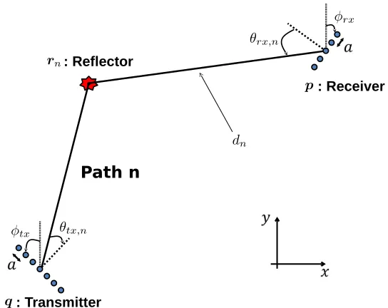
Npsignificant paths are received, where thenthpath geometry is seen in Fig. 2.2. The path begins at
the transmitter array located atqwith array orientation angleφtx, reflects at locationr, and ends
at a receiver array with locationpand array orientation angleφrx. The path geometry created by
the transmitter, reflector, and receiver locations dictate the parametersθtx,n: the angle of departure at the transmitter,θrx,n: the angle of arrival at the receiver, anddn: the total distance traveled by
the path from transmitter to receiver. It is noted that the path in Fig. 2.2 characterizes both LOS
and NLOS paths since a LOS path can be characterized by a reflector anywhere on the line segment
betweenqandp. The channel from (2.2) is expressed in terms of theNpsignificant paths[Sha18;
BS15]:
H[k] =
Np−1
X
n=0
hn(k)exp
−j2πkτn
TOFDM
arx(θrx,n)atx(θtx,n)H, (2.4)
wherehn(k)is the path loss andτn=dn/cis the time to travel from the center of the transmitter array
to the center of the receiver array, withc as the speed of light. It is assumed that both transmitter
frequency. Then, the beamforming vectorsarxandatxare:
arx(θrx,n) =
e−j2πλa Nrx2−1
sin(θrx,n)· · ·ej2πλa Nrx2−1
sin(θrx,n)T, atx(θtx,n) =
e−j2πλa Ntx2−1
sin(θtx,n)
· · ·ej2πλa Nrx2−1
sin(θtx,n)T
.
For sufficiently long symbols (TOFDM) the path loss coefficient is equivalent at each subcarrier[Sha18;
BS15]. Thus, it is assumed thathn(k)≈hnfor allk. This assumption is discussed in further detail in
Section 2.5.1.
By substitutingtn=dn/c in (2.4), it is seen that besides the path losshn, the channel is
com-pletely characterized by the channel parametersθtx,n,θrx,n, anddn:
H[k] =
Np−1
X
n=0
hnarx(θrx,n)atx(θtx,n)Hφ(dn)[k], (2.5)
where,
φ(dn)[k] =exp
−j2πk dn
c TOFDM
. (2.6)
2.2.2 Tucker Tensor Form
To be self-contained, we cover prerequisite tensor knowledge prior to showing that the received
sig-nal in a MIMO OFDM system naturally groups into a Tucker tensor form. Our notation is consistent
with[Sid17], which can also be referred to for further information. We first define the tensor product
or outer product. The third order tensor product is defined such that tensor elements resulting from
the product between the vectorsa,b, andcare(aýbýc)(i1,i2,i3) =a(i1)b(i2)c(i3). Tensor products of higher dimension follow similarly.
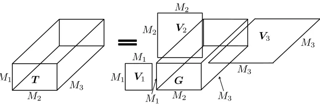
Any tensor can be represented in Tucker form. For a third orderM1×M2×M3tensorT, the Tucker form is[Sid17]:
T =
M1
X
i1=1
M2
X
i2=1
M3
X
i3=1
Path n
: Receiver
: Transmitter : Reflector
Figure 2.2Channel parameters for a path between the transmitter array and receiver array.
whereGis a core tensor, andV1,V2,V3are matrices composed of column vectors such thatV(:,i) is used to represent theithcolumn of matrixV. The core elementG(i1,i2,i3)corresponds with the strength of the interaction between columni1inV1, columni2inV2, and columni3inV3. Fig. 2.3
visualizesT as a series of vector tensor products. The Tucker tensor form in (2.7) can also be written
in a shorthand notation as follows:
T =G ý1V1ý2V2ý3V3, (2.8)
where ýi represents a tensor product along theithdimension with the core tensorG. Fig. 2.4
visualizes this form. Now that the Tucker form has been introduced, the following subsection shows
that the MIMO OFDM received signal naturally groups into a Tucker tensor form.
2.2.3 The Channel in Tucker Tensor Form
Channel estimation and localization are typically performed during a training sequence interval,
channel parameters. Without loss of generality, we letXbe all zero, besides ones on the diagonal.
SubstitutingX and the channel representation from (2.5) into (2.2), the received signal for each
subcarrier is
Y[k] =
Np−1
X
n=0
hnwa,n(θrx,n)fa,n(θtx,n)φ(dn)[k] +n[k], (2.9)
fork=1, . . . ,Nswhere
wa,n(θrx,n) =WHarx(θrx,n), (2.10)
and
fa,n(θtx,n) =atx(θrx,n)HF. (2.11)
A vector is created from the termsφ(dn)[k]that contains{φ(dn)[k]} Ns
k=1across all subcarrier frequencies:
φn(dn) =
h
1 e
−j2πdn
c TOFDM · · · e
−j2π(Ns−1)dn c TOFDM
iT
. (2.12)
Then, the measurement across all subcarrier frequencies can be constructed as a third-order tensor
with dimensionsLrx×NT×Nsas follows:
Y =
Np−1
X
n=0
hnwa,nýfaT,nýφn+n, (2.13)
which is now in Tucker form with rankNpas seen in (2.7), wheren∈CLrx×NT×Nsis the noise over all
subcarriers. It is noted that the dependencies of the vectors on the parametersθrx,n,θtx,n, anddn
have been dropped for simplicity in notation. The simplified Tucker form from (2.8) is obtained
by grouping the vectorswa,ninto the matrixWa= [wa,1wa,2 . . .], the vectorsfa,n into the matrix
Fa = [faT,1faT,2 . . .], and the vectorsφn into the matrixΦ= [φ1φ2 . . .]. Then, the measurement tensor is:
Y =Ψý1Waý2Faý3Φ+n, (2.14)
Figure 2.3Vector-wise outer product view of Tucker model.
This work focuses on third order tensors because we restrict paths to a plane and do not consider
elevation angles for simplicity. The result is a third order measurement tensor where the column
space corresponds with path AOA, the row space corresponds with path AOD, and the fiber space
corresponds with path distance. A model that allows a three-dimensional path and considers both
elevation angles and azimuthal path angles will lead to a five-dimensional measurement tensor. A
significant advantage of the Tucker form is that it extends to higher dimensions. All of the derivations
in this work are for three-dimensional tensors, but each step can easily be extended and applied to
higher order tensors for path models that also consider elevation angle.
Accurate estimates of the channel parametersθrx,n,θtx,n, anddnforn=0, . . . ,Np−1 enable a number of capabilities for 5G networks. The most obvious capability is channel estimation, since
H[k]can be reconstructed from the channel parameters for each subcarrier[Alk14]. Additionally, the channel parameters can be exploited to estimate the receiver position and NLOS path reflection
locations[RGn]. Thus, receiver localization and environmental mapping can be achieved with the
knowledge of these parameters, where environmental mapping is obtained when the NLOS path
reflection locations are estimated over several measurements. The estimate ofdnfromφncan also
be used to estimate the time delayτn between the transmitter and receiver, which can be used to
Figure 2.4Full Tucker tensor form.
2.3
Problem Formulation for mmWave Channel Parameter Estimation
We are interested in estimating the channel parametersθrx,n,θtx,n, anddn forn=0, . . . ,Np−1 as well as the path gainhnfrom the tensor form of the receiver measurementY of a training sequence
as in (2.14). This is accomplished by estimatingΨ,Wa,Fa, andΦ, which is the main goal of the rest
of this paper. A number of challenges make this a difficult task. For example, the number of paths
Npis unknown and must also be estimated. Additionally, this is a high dimensional problem and
the channel parameters must be estimated jointly.
Mathematically, since the measurement tensor is low rank, the channel parameter estimation
problem can be posed in the following form:
ˆ
Ψ, ˆWa, ˆFa, ˆΦ=arg min
Ψ,Wa,Fa,Φ
||Y −Ψý1Waý2Faý3Φ||2F
+λ||vec(Ψ)||0, (2.15)
where|| · ||0is thel0-norm (number of non-zero terms),λis a scaling parameter, andΨ,Wa,Fa,Φ
are functions ofhn,θrx,n,θtx,n, anddn respectively. The first term in (2.15) minimizes the Frobenius
norm of the error and the second term enforces low rank in the estimated tensor reconstruction.
The rank of the reconstructed tensor is the estimate for the number of paths and the second term
ensures that a minimal number of paths are used for channel parameter estimation. Section 2.4
of the channel parameters as well as the path gain in (2.13).
2.4
Multilinear SVD for mmWave Channel Parameter Estimation
The MSVD is an extension of the singular value decomposition to tensors and reconstructs a third
order tensor into a set of column, row, and fiber basis vectors. This section first introduces the
MSVD. Then, the MSVD of the third order measurement tensor is used to create a reduced rank
Tucker form and estimate the channel parameters. The properties of the MSVD are only minimally
covered here and further details can be found in[Sid17].
2.4.1 The Multilinear Singular Value Decomposition
The MSVD reconstructs tensors into a Tucker form, so that the interaction energy between basis
vectors is arranged in decreasing order. The MSVD of the received measurement tensor gives the
following Tucker form:
Y =Σý1U(1)ý2U(2)ý3U(3),
=
Lrx
X
i1=1
NT X
i2=1
Ns
X
i3=1
Σ(i1,i2,i3)u(i11)ýu
(2)
i2 ýu
(3)
i3,
(2.16)
whereu(i1)
1 =U
(1)(:,i
1),u(i22)=U
(2)(:,i
2), andu(i33)=U
(3)(:,i
3)are orthonormal basis column vectors such that(U(i))HU(i)=Ifori=1, 2, 3, whereIis the identity matrix. Each basis vector matrixU(i)
is square. The MSVD is arranged so that a majority of the energy is in the upper left corner of the
core tensorΣ, corresponding with the strongest interactions between sets of column, row, and fiber
vectors.
Singular values for the MSVD are defined such that each dimension of the core tensorΣhas its
own set of singular values. Thelthsingular value along the first dimension (or column space) is
defined as||Σ(l, :, :)||F, which is the Frobenius norm of the slab ofΣthat contains thelthcolumn.
other dimensions follow similarly.
It is noted that in the standard SVD, the column space and row space have the same rank.
However, in the multilinear SVD, the column, row, and fiber spaces can have different ranks. For
(2.16), the column rank is the number of columns inU(1), the row rank is the number of columns in
U(2), and the fiber rank is the number of columns inU(3).
2.4.2 Rank Reduction
It is known that few significant paths exist in the model from (2.13), which besides small noise
interactions, makesY a low rank tensor. On the other hand, the MSVD from (2.16) has a column
rank ofLrx(number of data streams), a row rank ofNT(number of training symbols), and a fiber rank
ofNs(number of subcarriers). A majority of the interactions from the MSVD must be eliminated
to obtain a low rank representation ofY. The strongest interactions mainly consist of energy
from significant received paths and the weakest interactions are mainly composed of energy from
non-significant paths and noise.
The rank of the MSVD (2.16) can be reduced by removing interactions that correspond with
singular values below a threshold in each dimension. This is achieved by removing planes from
Σs corresponding with the weak singular values along with the interacting row, column, and fiber
vectors. This acts as a denoising process[Hay17]and the remaining reduced rank Tucker form is
Y =Σsý1Us(1)ý2Us(2)ý3Us(3), (2.17)
where ifr1,r2, andr3are the reduced ranks of the column, row, and fiber subspaces; thenΣs is a
r1×r2×r3core tensor,Us(1)is aLrx×r1matrix,U( 2)
s is aNT×r2matrix, andU( 3)
s is aNs×r3matrix. A variety of methods can be used to select singular value thresholds. The aim is to select
thresholds such that the energy related to weak paths and noise are removed while the remaining
terms in (2.17) consist of energy from significant paths. The number of nonzero terms inΣs is an
Figure 2.5The measurement tensorY is sizeLrx×NT×NswhereLrxis the number of data streams,NTis
the number of training symbols, andNsis the number of subcarriers. The reduced rank Tucker form from the MSVD selects the strongest components from each subspace.
optimum threshold for each dimension issthresh=2.858smed, wheresmedis the median singular value along that dimension. We use this threshold value, but[GD14]discusses alternative thresholds.
Fig. 2.5 shows the reduced rank Tucker tensor form after thresholding.
2.4.3 Separating Channel Parameter Estimation into Separate Subspace Problems
The reduced Tucker form from the MSVD in (2.17) eliminates noise and estimates the number of
pathsNp, which is the rank of the measurement tensor. The denoised and rank reduced MSVD is
then approximately equivalent to the noiseless signal in the receiver measurement (2.14) :
Ψý1Waý2Faý3Φ≈Σsý1Us(1)ý2Us(2)ý3Us(3). (2.18)
Channel parameter estimation is accomplished by estimating the unknownΨ,Wa,Fa, andΦ
ma-trices. Assuming the reduced Tucker form from the MSVD sufficiently separates the noise from
the signal, the basis vectors in (2.18)Us(1),Us(2), andUs(3)share the same subspaces asWa,Fa, and
Φ, respectively. Furthermore, each of the subspaces are independent. Therefore, representing the
channel in Tucker form enables channel parameter estimation to be separated into three
indepen-dent sub-problems in the column, row, and fiber subspaces, which separately solve forθrx,n,θtx,n,
Figure 2.6A basis transformation converts from an orthogonal MSVD basis to a non-orthogonal dictionary basis.
Figure 2.7Overdetermined problem to compute the column subspace basis transformationQ1.
permutation ofθrx,n,θtx,n, anddnhas to be considered jointly.
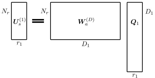
For the column subspace, the objective is to utilize the basis vectors fromUs(1)to estimateWa such that the columns ofWa correspond with physically realizable paths in the channel. This
equates to finding a value ofθrx,nfor each column ofWa. However, this is challenging since the basis vectors generated by the MSVD are not unique. Additionally, the basis vectors inUs(1)are
orthonormal while the true path column vectors inWaare not necessarily orthogonal.
formu-lated from physical paths exists as follows:
Wa(D)= h
ˆ
wa,n(θrx,1(D)) · · · wa,n(θrx,(DD)1)
i
, (2.19)
where{θrx,(Dm) }mD1=1is a set ofD1dictionary values and
ˆ
wa,n(θrx,i) =
wa,n(θrx,(Di))
wa,n(θrx,(Di))Hwa,n(θrx,(Di))
, fori=1, . . . ,D1
are normalized column vectors from (2.10), formulated from an over-complete dictionary ofD1
possibleθrx,nvalues. Fig. 2.6 shows an example with two basis vectors and two dictionary vectors.
In this example, the orthonormal basis vectors from the MSVDUs(1)do not align with possible basis
vectors inWa(D). Note that Fig. 2.6 is a projection into two dimensions while the actual basis vectors
are inNrxspace.
Estimating the columns ofWaessentially becomes a basis transformation where we seek the
basis transformation matrixQ1such that:
Us(1)=Wa(D)Q1. (2.20)
This is an overdetermined problem since the dictionary is overcomplete and there are many more
dictionary terms than paths (D1≥Np). Thus, the solution is not guaranteed to be unique. However, the measurement tensor is low rank and the solution forQ1must haver1nonzero terms to match
the rank of the column subspace. This leads to a sparse optimization problem, where the selection
of dictionary basis vectors is accomplished by enforcing sparsity onQ1. The row and column
subspaces follow similarly.
2.4.4 Subspace Estimation
Similar sparse estimation problems to (2.20) are posed in[Hay17],[Cot05],[Mal05]where sparsity is
inQ1by solving the optimization problem:
arg min Q1
||Us(1)−Wa(D)Q1||2F +λ||Q l2
1||1, (2.21)
whereλis a tuning parameter andQl2
1 is a vector containing thel2norm for each row ofQ1. Posing
the sub-problem in this form results in the multiple measurement vector sparse estimation problem.
Multiple solution techniques are discussed in[Cot05],[CH05], but we choose to use the multiple
measurement vector orthogonal matching pursuit (M-OMP) algorithm. M-OMP is chosen since it
is a greedy algorithm and requires less computation. Details on M-OMP can be found in[CH05].
The sparsity of the column subspaceQ1is set to the rank of the column subspace found from the
MSVD (r1), which is the number of columns inUs(1). The output of M-OMP isQ1withr1non-zero rows. This effectively eliminates all butr1dictionary vectors and allows the dictionary to be reduced
to the following:
˜
Wa(D)=Wa(D)A, (2.22)
where the reduced dictionary matrix ˜Wa(D)isNrx×r1andAis a sparse matrix identical toQ1, but with any non-zero rows replaced with a row of ones. Then the reduced dictionary is used in replacement
of (2.20) to obtain
Us(1)=W˜a(D)Q˜1, (2.23)
where ˜Q1is ar1×r1matrix. Note that selectingr1dictionary terms at this step significantly reduces future computational effort. Similarly, the row subspace uses a reducedr2×r2matrix ˜Q2and a
NT×r2matrix ˜Fa(D)such that
Us(2)=F˜a(D)Q˜2. (2.24)
The fiber subspace uses a reducedr3×r3matrix ˜Q3and aNs×r3matrix ˜Φ(
D)such that
At this point dictionary terms have been selected in each subspace. The transformation matrices
˜
Qi fori=1, 2, 3 contain information about how each of the dictionary vectors align with the MSVD
basis vectors, but dictionary vectors have not yet been explicitly chosen as estimates for the basis
vectors.
2.4.5 Super-Resolution Channel Parameter Estimation
The dictionaries used to obtain solutions to (2.23)-(2.25) may be coarse since the dictionaries are
limited in size. This is especially true since the computational effort of M-OMP increases with the
number of dictionary terms and smaller coarse dictionaries reduce computations. Higher resolution
can be obtained by iteratively updating the dictionary as strong dictionary terms are identified.
One approach for this is the K-SVD method, which is a dictionary learning algorithm that can be
employed with sparse problems[Aha06; Rub08]. We use K-SVD for our simulations as it significantly
reduced computation time when compared to a single large dictionary. Each iteration begins by
solving the sparse estimation problem with the last dictionary set. Then a new dictionary is created
that focuses around the dictionary terms chosen during the sparse step.
2.4.6 MSVD Basis Transformation
The best dictionary terms have been selected from (2.23)-(2.25) along with their transformation
matrices. These are now used to transform the MSVD in terms of the dictionary basis set in every
subspace. SubstitutingUs(1),Us(2), andUs(3)from (2.23), (2.24), and (2.25) into (2.17):
Y =Σsý1 W˜a(D)Q˜1
ý2 F˜a(D)Q˜2
ý3 Φ˜(
D)Q˜
3
. (2.26)
Or, equivalently:
Y =Σ0sý1W˜a(D)ý2F˜a(D)ý3Φ˜(
D), (2.27)
where
Σ0 =Σ
The tensor in (2.27) expressesY in terms of the basis created by the dictionaries in each subspace.
The core tensorΣ0s contains the interaction energy between the path channel parametersθrx,n,θtx,n,
anddnfrom the dictionary. However, it may not be obvious which path channel parameters have
the strongest interactions and should be linked together.
2.4.7 Linking Channel Parameters to Paths
It is known that the tensorY has rankNp. This low rank structure provides a means to select and
link the dictionary terms to paths. One may expectΣ0s in (2.27) to haveNpnon-zero terms. However, this is not guaranteed after the basis transformation as the dictionary vectors in each subspace are
generally not orthogonal. Therefore, we must eliminate interactions fromY so that it again has
rankNp. To do this, we select the dictionary terms with the strongest interactions inΣ0s. This is accomplished by first taking the MSVD ofΣ0s:
Σ0
s=Sý1D(1)ý2D(2)ý3D(3). (2.29)
The MSVD ofΣ0s results in the core tensorS, which organizes the interaction energies in decreasing order.
At this point the strongestNpelements inS correspond with theNppaths. It is noted that
distinct channel parameters for each path lead toNp=r1=r2=r3and the strongest interactions will be the diagional elements inS. However, there are scenarios when this is not the case. For
example, ifNp=2, but both paths have the sameθrx,nwith differentθtx,nanddnthenr1=1 while
r2=2 andr3=2. In this case, one of the strongest interactions will be off-diagonal inS. The method in[Zho17]does not offer a solution for this type of scenario since the CPD tensor form does not
allow multiple paths to share parameter vectors.
A significant advantage to the MSVD in (2.29) is that it provides a simple means to determine
the values ofθrx,n,θtx,n, anddnfor each path. In the form of (2.29) each column ofD(i)fori=1, 2, 3
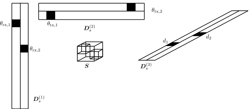
Figure 2.8Linking channel parameters for each path.
term is aligned for that subspace and path. Therefore, the channel parameters for each path are
estimated by choosing the maximum value in each column ofD(i)fori=1, 2, 3. Suppose that the
strongestNppaths inShave been chosen and the channel parameters are desired for pathnthat
correspond with the elementS(i1,i2,i3). Then, the channel parameters are found as:
m1=arg max
m D(m,i1),
m2=arg max
m D(m,i2),
m3=arg maxm D(m,i3).
(2.30)
As a result, the channel parameters for that path are:
θrx,n=θ˜rx,(Dm)1, θtx,n=
˜ θ(D)
tx,m2, dn=
˜
dm(D)
3 , (2.31)
where{θ˜(D)
rx },{θ˜
(D)
tx },{d˜(D)}are the set of dictionary terms from (2.23)-(2.25) with sizesr1,r2, andr3, respectively. An example of the path linking process is seen in Fig. 2.8. In this example, the strongest
two paths are the diagonal elements ofSs. The strongest elements in each column are selected and
Algorithm 1Channel Parameter Estimation:{θrx,n,θtx,n,dn,hn} Np
n=1=estMSVD(Y) 1)Take the MSVD of the measurement tensor:
Y =Σý1U(1)ý2U(2)ý3U(3)
2)Threshold the singular values and estimateNp:
Y ≈Σsý1Us(1)ý2Us(2)ý3Us(3)
3)Use K-SVD and M-OMP to solve for the dictionary vectors ( ˜Wa(D), ˜F(
D)
a , ˜Φ( D)
) and trasformation matrices ˜
Q1, ˜Q2, ˜Q3.
4)Convert the MSVD to dictionary basis:
Y =Σ0sý1W˜a(D)ý2F˜a(D)ý3Φ˜(
D)
5)Take the MSVD of the core tensor: Σ0
s =Sý1D(1)ý2D(2)ý3D(3)
6)Obtain(θrx,n,θtx,n,dn)forn=1, . . . ,Npby selecting the strongest elements inSalong with the maximum elements in the corresponding columns.
7)EstimatehnusingY and the estimated channel
parameters.
2.4.8 Estimating Path Gain
If desired, the path gain can be estimated for each path using the measurement vectorY and the
estimated channel parameters. This is done by vectorizing the measurement signal tensor as shown
in[Sid17]:
vec(Ψý1Waý2Faý3Φ) = (ΦFaWa)h, (2.32)
whereis the Khatri-Rao product andhis a vector of the path gains. LetA=ΦFaWa; then, the path gains are estimated by solving forhsuch that
arg min h
Y −Ah
2 . (2.33)