Scholarship@Western
Scholarship@Western
Electronic Thesis and Dissertation Repository
4-13-2017 12:00 AM
Patch-based Denoising Algorithms for Single and Multi-view
Patch-based Denoising Algorithms for Single and Multi-view
Images
Images
Monagi H. Alkinani
The University of Western Ontario
Supervisor
Prof. Mahmoud R. El-Sakka The University of Western Ontario
Graduate Program in Computer Science
A thesis submitted in partial fulfillment of the requirements for the degree in Doctor of Philosophy
© Monagi H. Alkinani 2017
Follow this and additional works at: https://ir.lib.uwo.ca/etd
Part of the Graphics and Human Computer Interfaces Commons, and the Other Computer Sciences Commons
Recommended Citation Recommended Citation
Alkinani, Monagi H., "Patch-based Denoising Algorithms for Single and Multi-view Images" (2017). Electronic Thesis and Dissertation Repository. 4465.
https://ir.lib.uwo.ca/etd/4465
This Dissertation/Thesis is brought to you for free and open access by Scholarship@Western. It has been accepted for inclusion in Electronic Thesis and Dissertation Repository by an authorized administrator of
In general, all single and multi-view digital images are captured using sensors, where they are often
contaminated with noise, which is an undesired random signal. Such noise can also be produced
during transmission or by lossy image compression. Reducing the noise and enhancing those
images is among the fundamental digital image processing tasks. Improving the performance of image denoising methods, would greatly contribute to single or multi-view image processing
techniques, e.g. segmentation, computing disparity maps, etc. Patch-based denoising methods
have recently emerged as the state-of-the-art denoising approaches for various additive noise
lev-els. This thesis proposes two patch-based denoising methods for single and multi-view images,
respectively.
A modification to the block matching 3D algorithm is proposed for single image denoising. An
adaptive collaborative thresholding filter is proposed which consists of a classification map and a
set of various thresholding levels and operators. These are exploited when the collaborative
hard-thresholding step is applied. Moreover, the collaborative Wiener filtering is improved by assigning greater weight when dealing with similar patches.
For the denoising of multi-view images, this thesis proposes algorithms that takes a pair of noisy
images captured from two different directions at the same time (stereoscopic images). The
struc-tural, maximum difference or the singular value decomposition-based similarity metrics is utilized
for identifying locations of similar search windows in the input images. The non-local means
algorithm is adapted for filtering these noisy multi-view images.
The performance of both methods have been evaluated both quantitatively and qualitatively through
a number of experiments using the peak signal-to-noise ratio and the mean structural similarity
measure. Experimental results show that the proposed algorithm for single image denoising out-performs the original block matching 3D algorithm at various noise levels. Moreover, the proposed
algorithm for multi-view image denoising can effectively reduce noise and assist to estimate more
To the woman who enfolds me—
MY PRECIOUS MOTHER, MALEHA,
who’s been the greatest, and most lasting teacher throughout my life,
and to
THE MEMORY OF MY FATHER, HASAN,
First and foremost, I would like to thank Allah for all his blessings to me. You give me each day the
power to undertake this work and complete it satisfactorily. I could never have done this without
your blessings, Almighty.
I would like to express my sincere appreciation to Dr. Mahmoud R. El-Sakka for his heartfelt guidance, assistance, and supervision to pursue my research. I am immensely grateful for studying
under each of your guidance.
I would like to thank my family for all endless encouragement while working on my thesis. Without
their love, tremendous support and patience, it would not have been possible to accomplish my
goals.
I acknowledge Jeddah University and the Cultural Bureau of Saudi Arabia in Canada for their
Abstract i
Epigraph iii
Dedication iv
Acknowledgements v
Table of Contents vi
List of Tables x
List of Figures xi
List of Algorithms xiv
List of Appendices xv
List of Abbreviations xvi
1 Introduction 1
1.1 Problem Background . . . 1
1.2 Problem Statement . . . 4
1.3 Research Purpose . . . 5
1.4 Research Objectives . . . 5
1.5 Research Methodology . . . 6
1.6 Thesis Structure . . . 7
2 Images Denoising: Background and Literature Review 8 2.1 Types of Noise in Digital Images . . . 8
2.2 Single Image Denoising . . . 9
2.3.2 Maximum a Posteriori-Markov Random Field . . . 52
2.3.3 A Statistical Approach with Adaptive NL-Means . . . 52
2.3.4 Discussion. . . 52
2.4 Additive White Gaussian Noise Estimating . . . 53
2.4.1 Spatial Domain Estimation Techniques. . . 53
2.4.2 Frequency Domain Estimation Techniques . . . 55
2.4.3 Discussion . . . 56
2.5 Images Similarity Measures. . . 56
2.5.1 Mean Square Error . . . 58
2.5.2 Peak Signal to Noise Ratio . . . 58
2.5.3 Normalized Cross-Correlation . . . 59
2.5.4 Mean Average Error . . . 59
2.5.5 Structural Content. . . 59
2.5.6 Maximum Difference . . . 60
2.5.7 Laplacian Mean Square Error. . . 60
2.5.8 Normalized Absolute Error . . . 60
2.5.9 Mean Structural Similarity . . . 61
2.5.10 Discussion . . . 62
2.6 Discretized Wavelet Transforms . . . 62
2.6.1 Haar Wavelet . . . 63
2.6.2 Meyer Wavelet . . . 65
2.6.3 Daubechies Wavelet. . . 65
2.6.4 Symlets Wavelet . . . 65
2.6.5 Coiflets Wavelet . . . 67
2.6.6 Biorthogonal and Reverse Biorthogonal Wavelets . . . 67
2.7 Review Summary . . . 70
3 Images Denoising: Empirical Results and Discussion 71 4 A New Patch-based Method for Single Image Denoising 78 4.1 Idea of the Proposed Method . . . 78
4.2 The Proposed Method . . . 81
4.2.1 Adaptive Collaborative Thresholding. . . 81
4.3.2 Parameters . . . 90
4.3.3 Transforms Selections . . . 90
4.4 Discussion . . . 91
5 New Patch-based Methods for Multi-view Image Denoising 94 5.1 Non-local Means for Multi-view Image Denoising . . . 94
5.2 Non-local Means with Structural Similarity . . . 96
5.2.1 Structural Similarity Index . . . 96
5.2.2 Full Searching. . . 97
5.2.3 Algorithm Outline . . . 97
5.3 Non-local Means with Differences Patch Similarity . . . 99
5.3.1 Patch Similarity Assessments . . . 99
5.3.2 Bounded Searching . . . 100
5.3.3 Algorithm Outline . . . 101
6 Results and Discussion 104 6.1 Image Similarity Measurements . . . 104
6.2 New Single Image Denoising Evaluation . . . 105
6.2.1 Quantitative Evaluation . . . 105
6.2.2 Qualitative Evaluation . . . 108
6.2.3 Discussion. . . 108
6.3 New Multi-view Image Denoising Evaluation . . . 108
6.3.1 Quantitative Evaluation . . . 111
6.3.2 Qualitative Evaluation . . . 113
6.3.3 Discussion. . . 119
7 Conclusions and Future Work 120 7.1 Summary of Contributions . . . 120
7.1.1 Single Image Denoising . . . 120
7.1.2 Multi-views Image Denoising . . . 121
7.2 Future Work . . . 122
Bibliography 123
Appendix D Discrete Wavelet Transforms Performances 139
2.1 Parameter set for the original block matching 3D filter . . . 44
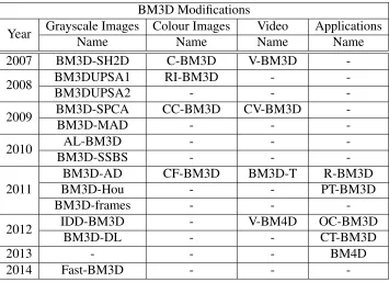
2.2 Block matching 3D filter modifications . . . 45
2.3 The properties information of the wavelet families . . . 64
4.1 Parameter set for our modified block matching 3D filter . . . 90
6.1 The performance of patch-based single image denoising methods . . . 107
1.1 Image denoising categories . . . 2
1.2 Detecting coins using active contours . . . 3
1.3 Disparity maps of stereoscopic images . . . 3
2.1 2D Gaussian distribution . . . 10
2.2 Gaussian filter with different sigma values . . . 12
2.3 The effect of the standard deviation values in Gaussian filter. . . 13
2.4 Robustness of the bilateral filter. . . 14
2.5 Bilateral filter with local image features . . . 15
2.6 Isotropic heat diffusion filtering . . . 17
2.7 Total variation method for image denoising . . . 20
2.8 The performance of theg(.) functions of the anisotropic diffusion filter . . . 22
2.9 The effects of number of iterations on anisotropic filtering . . . 23
2.10 The effects ofKon anisotropic filtering . . . 24
2.11 The effects ofλon anisotropic filtering . . . 25
2.12 NL-Means filtering strategy . . . 26
2.13 Weights distribution used in NL-Means filtering . . . 27
2.14 Probabilistic patch-based filtering scheme . . . 31
2.15 Dictionary learning filtering scheme . . . 33
2.16 Extracting patches in the PB-PCA . . . 36
2.17 Principal axes from the principal component analysis . . . 37
2.18 Comparison between using different shrinkage functions . . . 37
2.19 Collecting patches for PCA . . . 38
2.20 BM3D filtering scheme . . . 40
2.21 BM3D-SH2D and BM3D-SH3D flowcharts . . . 47
2.22 The iterative up-sampling scheme for BM3D-UPSA1 . . . 48
2.23 The iterative up-sampling scheme for BM3D-UPSA2 . . . 48
2.24 BM3D with shape-adaptive PCA scheme . . . 50
2.28 Single-level continuous and discrete 1D wavelet transform . . . 63
2.29 The wavelet functionΨof Haar transform . . . 64
2.30 The wavelet functionsΨof Meyer transform . . . 65
2.31 The wavelet functionsΨof Daubechies transform family . . . 66
2.32 The wavelet functionsΨof Symlets transform family . . . 66
2.33 The wavelet functionsΨof Coiflets transform family . . . 67
2.34 The wavelet functionsΨof Biorthogonal transform family . . . 68
2.35 The wavelet functionsΨof Reverse Biorthogonal transform family . . . 69
3.1 Low-pass filter vs. bilateral filter . . . 72
3.2 Isotropic heat diffusion and total variation filtering . . . 73
3.3 The four images used in patch-based image denoising experiment. . . 75
3.4 The performance charts when the noise is low (σ=20) . . . 76
3.5 The average consumed time charts . . . 77
4.1 Sorting patches based on range weights . . . 79
4.2 High textures image dataset . . . 80
4.3 Flat image dataset . . . 80
4.4 Denoising texture image by modified block matching 3D filter . . . 82
4.5 Denoising flat image by modified block matching 3D filter . . . 83
4.6 Modified block matching 3D filtering scheme . . . 84
4.7 The general scheme for texture analysis and thresholding . . . 84
4.8 Classification maps ofCameramanimage via various thresholds . . . 86
4.9 The six various thresholding levels . . . 87
4.10 The overall thresholding and training procedure . . . 88
4.11 Denoising using various wavelets at noise level (σ=10) . . . 92
4.12 Denoising using various wavelets at noise level (σ=30) . . . 93
5.1 Collecting similar patches from a stereoscopic image . . . 95
5.2 A full search for a rowtfrom the right stereoscopic imagetright . . . 97
5.3 Denoising stereoscopic image using structural similarity assessment with NL-Means 98 5.4 Bounded search for a rowtfrom the right stereoscopic imagetright . . . 101
5.5 Denoising stereoscopic image using MD or SVD-based similarity assessments . . . 103
6.1 Single image dataset. . . 106
6.6 Performance of patch-based multi-view image denoising methods . . . 113
6.7 Fragments of multi-view image denoising results . . . 114
6.8 Fragments of denoised multi-view image disparity maps. . . 114
6.9 Tsukubamulti-view image denoising results . . . 115
6.10 Tsukubamulti-view image denoising disparity maps . . . 115
6.11 Conesmulti-view image denoising results . . . 116
6.12 Conesmulti-view image denoising disparity maps . . . 116
6.13 Teddymulti-view images denoising result . . . 117
6.14 Teddymulti-view image denoising disparity maps . . . 117
6.15 Venus multi-view image denoising results . . . 118
2.1 Dictionary learning filtering method . . . 34
5.1 Denoising stereoscopic image using structural similarity with NL-Means . . . 98
Appendix A Performance results . . . 134
Appendix B Execution time . . . 136
Appendix C Thresholding levels and operators . . . 138
ADF Anisotropic Diffusion Filter
AWGN Additive White Gaussian Noise
BF Bilateral Filtering
BM Block Matching
BM3D Block Matching 3D
BM3D-Hou BM3D of Hou
BM3D-SAPCA Shape-Adaptive Principal Component Analysis BM3D-SH2D BM3D Sharpening 2D
BM3D-SSBS BM3D with Smooth Sigmoid Shrinkage function
BM3D-UPSA BM3D Iterative Up-sampling Algorithm
CPA Chebyshev Polynomial Approximation
CWT Continuous Wavelet Transform
DCT Discrete Cosine Transform
DL Dictionary Learning
DWT Discretized Wavelet Transform
EPLL Extend Patch Log Likelihood GLCM Grey-Level Co-occurrence Matrix
HSI Hyper-spectral Image
HT Hard Thresholding
HVS Human Visual System
It-PPB Iterative Probabilistic Patch-Based filter
K-SVD K-means Singular Value Decomposition
KoK Keep or Kill
LMSE Laplacian Mean Square Error
LPA-ICI Local Polynomial Approximation with the Intersection of the Confidence Interval MAE Mean Average Error
MSSIM Mean Structural SIMilarity
NAE Normalized Absolute Error
NCC Normalized Cross-Correlation
NL-Means Non-local Means
NLF Noise Level Function
Non-iPPB Non-iterative Probabilistic Patch-Based filter
PB-PCA Patch-based Principal Component Analysis
PCA Principal Component Analysis
PGPCA Patch-based Global PCA PHPCA Patch-based Hierarchical PCA
PLPCA Patch-based Local PCA
POL-SAR Polarimetric Synthetic Aperture Radar
PPB Probabilistic Patch-Based filter
PPBWE PPB Weights Estimator
PSNR Peak Signal-to-Noise Ratio
RGB Red, Green, and Blue
S-MD Non-local Means with Maximum Difference similarity for Stereo image denoising
S-SSIM Non-local Means with Structural similarity for Stereo image denoising S-SVD Non-local Means with SVD-based similarity for Stereo image denoising
SC Structural Content
SNR Signal Noise Ratio
SSBS Smooth Sigmoid Shrinkage Function
SSIM Structural SIMilarity
ST Soft Thresholding
Stereo-MSE Stereo denoising with Mean Square Error
SVD Singular Value Decomposition
SVD-based Singular Value Decomposition-based similarity assessment TV Total Variation
USC-SIPI University of Southern California-Signal and Image Processing Institute
WMLE Weighted Maximum Likelihood Estimation
Introduction
Dealing with random noisy pixels in an image is a major challenge for many image processing
applications due to the difficulty of distinguishing noise from true image information. Noise affects
all kinds of images whether they are single or multi-view. It also affects various types of image
areas, such as textured, flat or edge areas. Image denoising techniques, which can estimate the
true image pixels, are broadly grouped into two main approaches: pixel-based filtering and
patch-based filtering. A pixel-patch-based image filtering scheme is mainly a proximity operation used for
manipulating one pixel at a time (pixel-wise). It is based on examining spatial neighbouring pixels
located within a kernel. On the other hand, in patch-based image filtering, the noisy image is
divided into patches, or “blocks”, which are then manipulated separately in order to provide an estimate of the true pixel values (patch-wise). It is based on similar patches located within a search
window. Unlike pixel-based image filtering, patch-based and algorithms successfully utilizes the
redundancy and the similarity among the various parts of the input image to reconstruct a more
distinct image. The mechanisms of using these two methods are illustrated in Figure1.1.
1.1
Problem Background
Single and multi-view images are captured using sensors during the data acquisition phase. A single view image consists of one image; a multi-view image consists of two or more images,
which are generated simultaneously from different camera sources at different locations, and are
focused on one scene. These images are often contaminated with undesirable random noise during
(a) (b)
Figure 1.1: Image denoising categories: (a) filtering based on neighbouring pixels located within a kernel in pixel-based denoising schemes, and (b) filtering based on patches located within a searching window in patch-based denoising schemes.
Single images are used in diverse image processing applications, such as in object recognition, segmentation, and object tracking. Noisy single images exert significant influence on the
reliabil-ity of these applications. For insistence, when detecting non-smoothed objects in noisy images,
some algorithms may mistakenly detect disconnected objects due to the presence of noisy pixels.
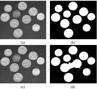
Figure1.2 shows the results of an attempt to detect coins using snakes active contours [59]. The
figure reveals that when noise contaminates the targeted objects “coins” they make it more diffi
-cult to produce reliable segmentations. Noise misleads the contours to not fit exactly onto object
boundaries, see Figure1.2(d).
Multi-view images have even more sophisticated imaging applications. These applications include
3D stereoscopic film, and the extraction of depth information. The quality of these applications
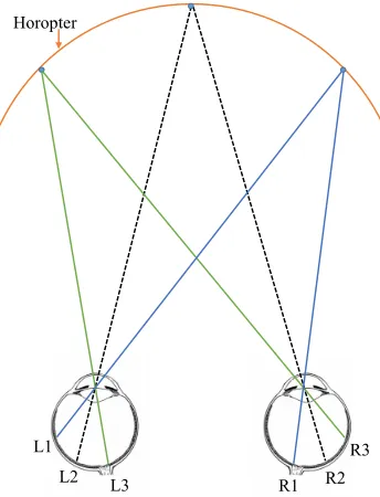
depends mainly on the image clarity. In support of this, the disparity maps1of a stereoscopic image both with and without noise were obtained using the graph-cut algorithm of Boykovet al. [16] in Figure1.3. When the stereoscopic image is corrupted by noise, the extracted depth information is
not clear, see Figure1.3(d).
The presence of noise in a single and/or a multi-view image has a significantly negative impact
on the results of various image processing applications. Hence, finding effective ways of reducing
noise in digital images is a very worthwhile area of research. Some noise reducing methods utilize
neighbouring pixels in order to estimate a centre pixel [104, 95]; however, such methods fail to
1The human brain process binocular disparity (the difference in image location of an object seen by the left and
(a) (b)
(c) (d)
Figure 1.2: Our results of detecting coins using snakes active contours of Kasset al. [59]: (a) noise-free image, and (b) the result of detecting coins using the noise-free image, (c) noisy image withadditive white Gaussian noise(σ=20), and (d) the result of detecting coins when noise is present.
(a) (b)
(c) (d)
research studies employ similar patches to restore a noise-free patch [17,32,61,24]. Such findings
benefit from the redundancy, which appears between patches, but they fail to properly preserve fine
details and smooth flat regions, and are very expensive in terms of time and memory when they are utilized for multi-view images. Thus, there is a need to develop a new patch-based image denoising
method, which has the ability to preserve fine details and smooth properly flat regions, for single
and multi-view images.
1.2
Problem Statement
TheBlock matching 3D(BM3D) filtering algorithm of Dabovet al. [24] is a patch-based denoising method, which depends mainly on the transformation coefficient thresholding procedure. When transferring a signal into the frequency domain, noise is characterized by low amplitude levels.
The BM3D filtering algorithm uses a fixed thresholding operator to force all of the coefficients
below the threshold to be zeros. This algorithm is considered to be a state-of-the-art denoising
method. Yet this method has several disadvantages, such as that of the difficulties related to the
choosing an optimal thresholding operator. When Marc Lebrun [64] described the influence of
all of the twenty parameters of the BM3D, he concluded that the thresholding operator is one of
the most important parameters of the BM3D because it controls the amount of the coefficient’s
thresholding level of the 3D patches group. Although previous researchers have shown ways of
optimally adjusting the BM3D parameters, they have not shown them bing used as an adaptive thresholding operator with a textures classification map which considers geometric and luminance
similarity distances. This study will address this classification map, in order to find an effective
way of enhancing single view images.
In the case of multi-view image denoising, various image similarity measures will be addressed;
these include maximum difference, structural similarity [97], and singular value decomposition
similarity [79] measures, in order to identify similar search windows among the multi-view images.
Thenon-local means(NL-Means) algorithm of Buadeset al. [17] will then be adapted for multi-view image denoising.
The research objective is therefore to investigate whether improving the means of optimizing the
thresholding operator could improve the overall ability of the BM3D method while preserving de-tail and suppressing noise in single view images. In addition, weight assignment for the Wiener
Fi-nally, the effectiveness of adapting a NL-Means filtering algorithm using various image similarity
measures for denoising multi-view images will be studied.
1.3
Research Purpose
Evaluating the geometric and luminance similarity distances between neighbouring pixels assist
the pixel-basedbilateral filterof Tomasiet al.[95] to optimally adjust the required weights before averaging pixels. By considering both similarity distances, this pixel-based filter preserves the
desired detail and suppresses more noise. Hence, adapting this idea to the patch-based BM3D
filter when thresholding the 3D group coefficients, we can preserve more detail and can suppress
more noise in a noisy single view image if the differences between flat and textured areas were considered.
Increasing the number of similar patches before thresholding or averaging improves the eff
ective-ness of the overall denoising procedure of the patch-based image denoising methods. Thus, instead
of denoising each view separately in a multi-view image, this study extends the search window to
use more reliable patch similarity measures in order to cover the entire spectrum of multi-view
im-ages. The effectiveness of several image similarity measures is examined to identify the location
of similar windows.
1.4
Research Objectives
The objective of this research is to develop effective approaches for denoising single and
multi-view digital images that fulfill the following requirements:
1. Exceed the performance of existing single and multi-view image denoising methods,
(a) quantitatively via:
i. Thepeak signal-to-noise ratio(PSNR).
ii. Themean structural similarity(MSSIM) of Wanget al.[97]. (b) qualitatively via:
i. The preservation of textures and fine details.
denoising methods (via disparity maps).
3. Produce a solution with simple computational complexity when denoising multi-view im-ages (via bounded searching areas).
By meeting these objectives, effective enhanced single or multi-view images would be achieved.
1.5
Research Methodology
In this section, the datasets and the techniques used to check the validity and reliability of this
work are described. Two image databases were used to evaluate the performance of the denoising
methods: a single image database, and a multi-view image database.
The single image dataset contains images obtained from the image database of the University of Southern California-Signal and Image Processing Institute (USC-SIPI) [1]. The USC-SIPI’s database has more than 237 images, but this research uses only ten images that were used in the
original BM3D research. This research ensured that the chosen images contain fine details, sharp
edges, grey gradations and pattern repetitions. The fine details of the Lena, Barbara, Man, and
Boats images were helpful in demonstrating how the various methods can preserve the image clarity; whereas the sharp edges of theHouseandCameramanwere helpful in demonstrating how the various methods can preserve the edges. The grey gradations ofHillimage provided insight into the amount of smoothing that has been applied to the images, and the Fingerprintimage assisted in revealing how pattern repetitions were preserved by the various methods.The size of the
single view images varies, e.g., 256×256 pixels, or 512×512 pixels. And they are all grey-scale
images. That is, they have 8 bits per pixel.
A collection of multi-view images from the stereoscopic database of Middlebury Computer Vi-sion[3] was used to evaluate the multi-view image denoising methods. Middlebury stereoscopic database has 71 images, but four multi-view images were used in this work. The images have been
carefully chosen to assist in distinguishing between the qualities of output from the various
details. The size of the images varies, e.g., 450×375 pixels, 434×383 pixels, or 384×288 pixels.
And they are all grey-scale images represented as 8 bits per pixel.
The image datasets were corrupted using additive white Gaussian noise (AWGN) with a noise variance that ranged from 10 to 100σ. The denoising methods then were employed to estimate the free of noise (a true image). This thesis exploits full reference similarity measures. The reference
image is assumed to be in existence and free of noise, as compared with the denoised image.
1.6
Thesis Structure
This thesis contains six chapters and three appendices. In Chapter 1, an introduction to image
denoising is introduced. In Chapter2, the background and the literature review on the subject of
image filtering are explained. In Chapter3, the empirical results and discussion are produced. In Chapter 4, the proposed patch-based denoising method for single image denoising is presented
and discussed. In Chapter5, patch-based denoising methods for multi-view image denoising are
presented and clarified. In Chapter 6, an empirical evaluation and the results of the denoising
methods are provided. In Chapter7, the conclusions and a perspective on the need for future work
on the subject of developing new patch-based image denoising methods are addressed. Finally,
Images Denoising: Background and
Literature Review
In this chapter, a general introduction to digital image denoising is presented. This chapter is
divided into five sections. In Section2.1, the main noise models are presented. In Section 2.2, a
background on single image filtering is introduced. In Section 2.3, a background on multi-view
image filtering is provided. Finally, the image similarity measurements are described in Section
2.5.
2.1
Types of Noise in Digital Images
Noise in digital images could be additive, multiplicative, or a mixture of such errors occurring in
the original signal. Additive noise is an interference added to the signal image pixel. Such noise in
a digital image is generally modelled as
υ(x)=u(x)+n(x)d,x∈Ω, (2.1) whereυ(x) is the noisy component of the image,u(x) is the true image,n(x)dis the random additive noise, andΩdenotes the set of all pixels in the image. In particular, ifn(x)d is a Gaussian random process, the noise is identified as Gaussian noise.
into the signal. Multiplicative noise in a digital image is modelled as:
υ(x)=u(x)×n(x)m,x∈Ω (2.2) where υ(x) is the noisy component of the image, u(x) is the true image, n(x)m is the random multiplicative noise, andΩdenotes the set of all pixels in the image.
The combination of the additive and multiplicative noises is called mixed noise. Mixed noise in a
digital image is modelled as:
υ(x)= n(x)m×u(x)+n(x)d,x∈Ω (2.3) whereυ(x) is the noisy component of the image,u(x) is the true image,n(x)dis the random additive noise,n(x)mis the random multiplicative noise, andΩdenotes the set of all pixels in the image. Image denoising methods can be categorized into two main groups: single image denoising
meth-ods and multi-view image denoising methmeth-ods. While one image is processed in a single image denoising process, multiple images are processed in a multi-view image denoising process.
2.2
Single Image Denoising
2.2.1
Pixel-based Image Filtering
In this subsection, a short background on pixel-based image filtering, which is an operation used
for manipulating one pixel at a time, is provided. Through the filtering process, a revised pixel
value is calculated using coordinates that are equal to the coordinates of the centre of a kernel. The
new pixel value is the result of the filtering process. When the centre of the filter visits each pixel
of the input image, a filtered image is generated. Linear filters then replace each image pixel with
a linear combination of its neighbours. Otherwise, the filter is called a nonlinear filter.
Figure 2.1: 2D Gaussian distribution with mean (0,0) andσ=1
ˆ
u(x,y)= a X i=−a
b X j=−b
I(x+i,y+ j)·H(i, j) (2.4)
2.2.1.1 Low-pass Filtering
Since noise in digital images is considered to be a high frequency component, applying low-pass
filters can eliminate noise in such images. The strength of the filters is related to the kernel sizes
and weights. There are several low-pass filters, e.g., mean, Gaussian and Yaroslavsky filters.
• Mean Filter: A mean filter replaces each pixel value with the average value of itself and its neighbours. By considering Equation2.4, the kernel of the mean filtering for an image is
provided in the expression:
H(i, j)Mean =
1
m×n (2.5)
• Gaussian Filter: A Gaussian filter is similar to the mean filter, but it uses a kernel that represents the shape of a Gaussian hump. A Gaussian filter could be described as a weighted average filter of the nearest pixels’ neighbours. Thus, it produces a smoother image than
that produced by a similarly sized mean filter. The definition of the weight is the main issue
to be addressed in averaging an additive noise for denoising. The weight in a Gaussian
filter is defined locally based on the neighbouring pixel’s location. The weights increase
when neighbours are closer to the central pixel’s location. The 2D Gaussian distribution
H(i, j)Gaussian has the form of Equation2.6; the weight depends on the geometric distance between pixels,
H(i, j)Gaussian =
1
√
2πσd
e−
|i−j|2
2σ2
d (2.6)
wherei, jare the coordinates of a pixel (i, j∈Ω),σdis the standard deviation of the Gaussian hump that determines the degree of similarity between spatially close pixels. The ideal
Gaussian filter has the property of having values less than one standard deviation from the
mean represents about 68.3% of the data under the Gaussian hump; two standard deviations
represent about 95.5% of the data, and three standard deviations represent about 99.7% of the data. The standard deviation of the Gaussian filter controls the degree of smoothing.
The standard deviation value is associated with the kernel size. A high standard deviation
value with a small kernel size makes a Gaussian filter behave more like a mean filter, and
hence it produces more smoothing of the edges. Figure2.2shows deploying various standard
deviations (σ) for denoising Lenaimage contaminated with AWGN. The edges are blurred when high values are used for the standard deviation with the same kernel size. The plot in
Figure2.3illustrates the effect of the Gaussian filters that are used in Figures2.2(d), (e) and
(f) on preserving edges. The grey values of the columns, which range from 105 to 150 in
row 150 ofLenaimage, are plotted in order to provide a visualization of the amount of edge blurring. From the plot, the edges are blurred as the standard deviation value increases.
• Yaroslavsky Filter: With a Yaroslavsky filter [104], the pixels are restored using the weighted average value of the pixels with similar grey level values within the same spatial neighbour-hood. This type of filter is an image-dependent filter; hence, the weights cannot be defined
using an image independent kernel. If we have a spatial neighbourhood in a kernel of size
n×m, the Yaroslavsky filter is defined as the formula shown in Equation2.7,
H(I(x,y),I(i, j))Yaroslavsky =
1
√
2πσr
e−
|I(x,y)−I(i,j)|2
2σ2
r (2.7)
whereI(x,y) andI(i, j) are the grey levels at two positions, andσris the standard deviation of the Gaussian hump that determines the degree of similarity between the grey levels.
2.2.1.2 Bilateral Filtering
(a) (b) (c)
(d) (e) (f)
105 110 115 120 125 130 135 140 145 150 0 50 100 150 200 250
Columns from 105 to 150 in Lena image (row = 150)
Pixel Grey Value
Original Image Noisy Image
σ = 1.66
σ = 3.33
σ = 6.66
(a) (b)
Figure 2.3: The effect of the standard deviation values of the Gaussian filters used in Figure2.2: (a) position of the columns from 105 to 150 in row 150, and (b) plot of the grey values of the columns.
filter is based on the geometric distance between pixels, the weighted average in a Yaroslavsky filter
is based on the luminance distance between pixels. BF utilizes these two distances, and assigns
higher weight to similar pixels. Hence, the weight of two pixels could be similar if they were to be
spatially located within the same distance from the centre pixel and they would have perceptually
similar values.
Since BF measures the geometric distance similarity using Equation 2.6and the luminance
simi-larity using Equation2.7for computing weights, the BF is shown as:
ˆ
u(x,y)= a X i=−a
b X j=−b
I(x+i,y+ j)·H(i, j)Gaussian·H(I(x,y),I(i, j))Yaroslavsky (2.8)
The weightH(I(x,y),I(i, j))Yaroslavsky prevents averaging across edges. The pixels belonging to the
same region are weighted averages, if the grey level difference between the two pixels is small.
Therefore, the BF does not blur the edges. The BF has the ability to average across features that
are located within 2σd from the centred pixel while preserving the fine details. Figure2.4 shows
the robustness of a BF in preserving the fine details.
The run-time of BF limits its usefulness in real-time. The BF is ineffective in smoothing regions
with high gradients; Figure2.5 (a) provides an example of such signals. BF fails when there are
not enough pixels to average. For example, presume that the grey level of a local neighbourhood
(a) (b) (c)
Figure 2.5: BF in one-dimensional signals of different local neighbourhood grey levels: (a) area with high gradient, (b) area with ridges and valleys, and (c) disjoint region. Where S is the geometric distance simi-larity and R is the luminance simisimi-larity range.
non-adaptive spatial filter, Figure2.5(c) shows that the BF fails to separate the disjointed regions.
The BF cannot be effectively adapted to filtering out these local features. All of the filters addressed
so far in this subsection (Subsection section2.2.1) are non-iterative filters, which produces a result
in a single pass. All of the remaining filters are iterative filters.
2.2.1.3 Variational Denoising Methods
The goal of variational denoising methods is to minimize the high level of energy in noisy images.
In order to minimize the high level of energy, regularization in variational denoising permits the
se-lection of the most reasonable solution from a group of several solutions. By assumingυ(x,y) is a noisy image andE(υ) is the energy that describes the quality of the image, the energy minimization process to estimate the original image ˆu(x,y) is defined as:
ˆ
u(x,y)= arg minE(υ) (2.9) Finding the local minimum of the energy in Equation 2.9 can be achieved by using a gradient descent optimizer. The gradient descent optimizer is an optimizer that takes a small step toward
the negative direction of the energy gradient (−∇E). The gradient descent is defined as: ˆ
• Isotropic Heat Diffusion: A sudden increase in a pixel value indicates a noisy pixel. Thus, the gradient|∇υ(x,y)|is expected to be high near a noisy pixel. In order to smooth the gradient values, the isotopic heat diffusion equation could be used as the energy to be minimized.
The heat equation is a parabolic partial differential equation, used to describe the behaviour
of the heat distribution in a region over time. Ifq(x,y) is a function of two spatial variables (x,y) andtis the time variable, the heat equation formula is formalized as:
∂q
∂t −α
∂2q
∂x2 +
∂2q ∂y2
!
= 0 (2.11)
whereαis a positive constant that controls the amount of the applied diffusion, and∂∂x2q2 +
∂2q
∂y2
is the laplacian operator (4q). The heat equation diffuses equally into all directions. Thus, it is called an isotopic diffusion equation. For the filtering of a noisy imageυ(x,y), Equation
2.11is used as the energy gradient function∇E optimized by the gradient descent shown in Equation2.10. The heat diffusion energy for the image is discretized as:
∇E =4υ = ∇xxυ(x,y)t +∇yyυ(x,y)t
(2.12)
where∇xxυ(
x,y)t and∇yyυ(
x,y)tare:
∇xxυ(x,y)t ≈ υ(x+1,y)t−2υ(x,y)t+υ(x−1,y)t
∇yyυ(
x,y)t ≈υ(x,y+1)t−2υ(x,y)t +υ(x,y−1)t (2.13) The heat diffusion imparts more smoothing to the image as the step size or the number of
iterations increases. The minimization process may fail to converge to a local minima when
using large step sizes. It is recommended that the step size be (0≤ 4t≤1/4) [83]. Figure2.6
shows the result of using various steps sizes along with the isotopic heat diffusion for image
filtering. In order to prevent smoothing across edges, a condition is needed to force the heat equation to be ∂υ∂t =0 near boundaries. Atotal variation(TV) filter uses a data fidelity term to overcome this problem.
• Total Variation: Rudinet al. [90] introduced the TV regularization for image denoising. The TV method is an edge-preserving denoising method. The TV method consists of two terms:
a regularization term and a data fidelity term. The regularization term assists in smoothing
flat regions, while the data fidelity term is used as a condition to prevent the smoothing of the
(a) (b)
(c) (d) (e)
(f) (g) (h)
arg min
υ T V|{z(υ})
Regularization Term
+ λ · |u−υ|2
| {z }
Data Fidelity Term (2.14)
whereT V(υ) indicates the TV andλ >0 is a parameter that balances the importance of the two terms in order to control the degree of filtering. The numerical approximation of the
energy shown in Equation2.14is:
∇E = 1
h ∇x
+υ(x,y)t q
∇x
+υ(x,y)t2+ m ∇y+υ(x,y)t,∇y−υ(x,y)
t2 (2.15) +
∇y+υ(x,y)t
q
∇y+υ(x,y)t2+
m ∇x
+υ(x,y)t,∇x−υ(x,y)
t2
−λt υ(x,y)t−υ0(x,y)
here, the neighbour differences `
are computed as
∇+xυ(x,y)t ≈ υ(x+1,y)t−υ(x,y)t (2.16)
∇−xυ(x,y)t ≈ υ(x−1,y)t−υ(x,y)t
∇y+υ(x,y)t ≈ υ(x,y+1)t−υ(x,y)t
∇y+υ(x,y)t ≈ υ(x,y−1)t−υ(x,y)t
m(·) is computed as
m(A,B) = minmod(A,B) (2.17) = sgn A+sgn B
2
λt = h 2σ2
X
(x,y)
q
∇x
+υ(x,y)t2+ ∇y+υ(x,y)t2 ! (2.18) − ∇x
+υ(x,y)0+∇x+υ(x,y)t q
∇x
+υ(x,y)t2+ ∇y+υ(x,y)t2 −
∇y+υ(x,y)0+∇y+k·υ(x,y)t
q
∇x+υ(x,y)t2+ ∇y
+υ(x,y)t2
whereσis the noise estimated variance andh, is the number of neighbours, which is equal to 4 for the 4-nearest neighbours or to 8 for the 8-nearest neighbours.
For image filtering, the energy function shown in Equation2.15is optimized by the gradient
descent shown in Equation 2.10. In order to analyze the energy convergence in the TV
method, two types of convergence are used with the gradient descent optimization in this
thesis. One of the convergences utilizes a fixed number of iterations, while the rest of the
convergences automatically calculates the number of iterations using the the mean square error as a condition. The automatic convergence stops if the mean square error between two iterations is less than 0.01, which means there is no visual quality improvement could
be achieved. The results of utilizing the two convergence types for the denoising ofLena
image are shown in Figure2.7. Figures2.7(c), (d), and (e) show that increasing the iteration
numbers imparts more smoothing to the images. Figures 2.7 (f), (g), and (h) show that
textures are blurred when theλvalue decreases.
2.2.1.4 Anisotropic Diffusion Filtering
Theanisotropic diffusion filter(ADF), introduced by Perona and Malik [83], iteratively blurs the non-edge regions while keeping the edges and the boundaries sharp. The ADF does not
ap-ply smoothing the same way in different directions; thus, it is called an-iso-tropic method. The
anisotropic diffusion equation for image denoising is defined as
ˆ
(a) (b)
(c) (d) (e)
(f) (g) (h)
wheredivindicates the divergence operator,ais the Laplacian operator,`is the gradient operator andtis a time scale. Equation2.19would be reduced to being an isotropic heat diffusion equation, ifc(x,y,t) were to be constant. It is worth mentioning that the smoothing amount is controlled by the value ofc(x,y,t). Perona and Malik attempted to automatically set the c(x,y,t) values to be close to 0 to prevent any smoothing across boundaries and to be close to 1 in smoothing the interior
regions. Equation2.19can be discretized on 4-nearest neighbours as
ˆ
u(x,y)t+1 = uˆ(x,y)t +λ
cN(x,y) t
· ∇−xυ(x,y)t+cS(x,y) t
· ∇+xυ(x,y)t +cE(x,y)
t
· ∇y+υ(x,y)t+cW(x,y) t
· ∇y−υ(x,y)t
(2.20)
where 0 ≤ λ≤ 1/4is used for stability,∇x
−, ∇
x
+,∇y−and∇
y
+are the neighbour differences computed as Equation2.16, andCN,CS, CE andCW are the conduction coefficients of the four neighbours for eachtiteration at the location (x,y). The conduction coefficients are defined as
CN(x,y)t =g k ∇x−υ(x,y)
t k
CS (x,y) t =
g k ∇+xυ(x,y)t k
CE(x,y)t =g k ∇ y
+υ(x,y)t k
CW(x,y)t =g k ∇ y
−υ(x,y)
t k
(2.21)
whereg(·) function is defined as
ghI= e−k
`
Ik/K2
(2.22)
or
ghI= 1
1+k∇KIk2
(2.23)
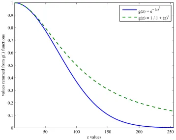
whereKis a constant that represents the noise standard deviation. g(·) function (Equation2.22) is the Taylor approximation ofg(·) function (Equation2.23). Both functions perform similarly. The plot provided in Figure2.8illustrates the performance of the two functions when the inputs were
0-255. Figure2.9shows the effects of the number of iterations on the ADF when used for denoising
50 100 150 200 250 0
0.1 0.2 0.3 0.4 0.5 0.6 0.7 0.8 0.9 1
z values
values returned from g(.) functions
g(z) = e− (z)
2
g(z) = 1 / 1 + (z)2
Figure 2.8: The performance of theg(.) functions (Equation2.22and Equation2.23) of the ADF.
2.11. When theλvalue increases, more smoothing is applied to the image.
2.2.2
Patch-based Image Filtering
It is now common practice in image denoising to utilize patch-based models and algorithms in-stead of pixel-based approaches to produce most promising estimate of the noise-free images.
However, there are advantages and disadvantages to the use of patch-based models and algorithms.
Among the advantages, the smoothing of flat regions is the most important. Redundancy between
patches enable patch-based approaches to properly smooth flat regions. Another advantage is the
preservation of fine image details and sharp edges. Among the disadvantages, the similarity
be-tween patches assists in estimating flat region, and so is averaging, but it is quite time-consuming
to group and compare similar patches. Therefore, each patch could have multiple estimates and
patches are overlapped. Secondly, while it may be that patterns and textures are seemingly clear,
patch-based models and algorithms usually exploit a large number of parameters, which can be
(a) (b)
(c) (d)
(e) (f)
(a) (b)
(c) (d)
(e) (f)
Figure 2.10: The effects of K on ADF: (a) an original Lena image, (b) an AWGN noisy
(a) (b)
(c) (d)
(e) (f)
Figure 2.11: The effects of λ on ADF: (a) an original Lena image, (b) an AWGN noisy
(a) (b)
Figure 2.12: Similarity between patches: (a) NL-Means patches as a raster scan in a search window, and (b) Patch P3 is more similar to P1 than to Patch 2; hence, P3 will receive a higher weight than the P2 weight.
Regardless, we believe that the advantages of patch-based methods far outweigh their
disadvan-tages, as modern computers are significantly overpowered, and have large memory banks.
2.2.2.1 Averaging Patch-Based: Non-local Means
NL-Means is a patch-based filter proposed by Buadeset al. [17] as a modification of the pixel-wise BF [95, 85, 13, 37,68, 99]. Like the BF, the NL-Means filter blurs homogeneous areas and
preserves edges. The NL-Means filter divides the input image into sub-images and then filters each
sub-image separately in patch-wise fashion. Each sub-image contains several patches. As in the
BF, similarity is measured based on two measurements: (1) the Euclidean distance between the
centres of the patches, and (2) the luminance distance between the patches. In contrast to the BF,
patches are compared within a searching window instead of with the pixels of its neighbours. Thus, it is called a non-local method. Patches with similar grey scale levels have larger weights when
they are averaged. Figure2.12 (a) shows the NL-Means patches and how to find similar patches
in a raster scan search window. Figure 2.12 (b) illustrates that patches with a similar grey scale
level, for example, P1 and P3, should be assigned a higher weight over those assigned to P1 and
P2. Figure2.13shows the weight range from 1 (white) to zero (black) for the displayed image; 1
indicates that there are two identical patches, and vice versa. The edges in NL-Means filtering are
preserved regardless of their direction.
Image Weight Image Weight Image Weight
(a) (b) (c)
Image Weight Image Weight Image Weight
(d) (e) (f)
Figure 2.13: The weights distribution used to estimate the central pixel of each searching window in NL-Means. The weights range from 1 (white) to zero (black) [17].
NL[v]i = X
j∈I
ω(i, j) [v]j (2.24) where [v]i and [v]j are pixel intensities at location i and j, respectively, and ω(i, j) is a similar-ity measure between the pixels iand j. The similarity measure of weight satisfies the condition 0 ≤ ω(i, j) ≤ 1 andP
jω(i, j) = 1. The similarity weight depends on the grey scale level’s simi-larity and the Euclidean distance between vectors N[v]iandN[v]j, whereN[v]k denotes a square neighbourhood of a fixed size and centred at a pixelk. The weights are described as,
ω(i, j)= 1
Z(i)e
−k
N[v]i
−N[v]j
k2
h2 (2.25)
whereZ(i) is a normalization factor andhis a filtering parameter set depending on the noise level. The level of noise determines the size required for the search windows and patches. For a ro-bust comparison between patches, the size of the patches increases when the noise level is high.
Accordingly, the value of the filtering parameter,hincreases as the size of the patch is increased. Meanwhile, the size of the search windows must be increased in order to find more similar patches.
The NL-Means filter has many modifications. Improving the weight assignment between the
patches improves the performance of the NL-Means method. Hedjam et al. [48] improved the process of adjusting the weights in the NL-Means by using Markovian clustering. Wu et al.
pre-classification strategy for optimizing the weight kernels of NL-Means filter. Khanet al. [60] introduced a variant of the NL-Means scheme by using a thresholding step to reduce the number
of similar patches before the weighted averaging of the patches.
The NL-Means filter exists in the spatial domain. Applying this filter in the frequency domain
would assist in suppressing a noisier signal. Alfredoet al. [38] transferred the patches of the NL-Means to the frequency domain, and used discrete cosine transform(DWT) with a set threshold to estimate true patches. Zhong et al. [109] combined the NL-Means with a Lee filter [65] for SAR images enhancing. Chan et al. [18] incorporated a median filtering operation indirectly in the NL-Means method for denoising low signal noise ratio (SNR) images. Maruf et al. [75] projected NL-Means patches into a global feature space before performing a statistical t-test to reduce the dimensionality of this feature space. Irreraet al. [54]adapted NL-Means for denoising X-ray images (XNLM), and then applied an additional multiscale contrast enhancement stage in the frequency domain.
An NL-Means filter could be adapted to improve other image processing applications (e.g.
seg-mentation, recognition, and video denoising). Zhan et al. [105] introduced an extension to the NL-Means method for ultrasonic speckle reduction. They assigned the patches’ similarity weights
iteratively in a lower dimensional subspace using principal component analysis(PCA). Xuet al.
[103] adapted the NL-Means for microscopy cell images using a frequency transform. Geninet al.
[42] adapted a modified version of the NL-Means filter for detecting small objects by background
suppression. Background pixels were estimated by applying a weighted average depending on the
similarity between the neighbouring pixels. Kimet al. [61] adapted the NL-Means filter for noise reduction and the enhancement of extremely low-light video. They use a motion adaptive temporal
filter using Gamma correction with adaptive thresholds before using the NL-Means filter. Xuet al.
[102] adapted the idea of patching from the NL-Means for filteringpolarimetric synthetic aperture radar(POL-SAR) images; they used simultaneous sparse coding for the transferring of the patches into the frequency domain before assigning the weights.
2.2.2.2 Probabilistic Patch-Based Filtering
The probabilistic patch-based filter (PPB) of Deledalle et al. [32], which works in the spatial domain, is an extension of the NL-Means filter. The PPB approach is one of the few denoising
techniques that can provide a general denoising methodology for various noise models. Thus, it is
multi-plicative speckle noise. The PPB filter is a statistically-based similarity scheme that depends on the
distribution model of the noise. The weighted average is used for the Gaussian noise distribution
in the NL-Means, but the PPB filter applies smoothing based on themaximum likelihood estimator
(MLE). The PPB is expressed as a weighted maximum likelihood estimation (WMLE) problem. The weight is derived from the data by improving the isotropy of the filter - non-iterative PPB filter(Non-iPPB), and it can be iteratively defined based on the similarity of the patches -iterative PPB filter(It-PPB).
Weighted Maximum Likelihood Estimator: UsingweightedMLE for image denoising is not a new technique; it was first used for image denoising by Polzehl and Spokoiny [88,87]. The PPB
filter redefined the weights in terms of a patch-based approach. This form of image denoising is
considered to be an estimation ˆuof the true imageuwhich originates from the noisy imageυ. The images are defined over a discrete regular gridΩ. A pixel value is described asi, and its neighbour is jat the location (x,y) ∈ Ω. The noise model is considered as being defined by the parametric noise distribution “likelihood” p(i | θ∗
i), where θ
∗
i is an unknown space-varying parameter. The denoising of an image is equivalent to finding the best estimation ˆθi forθ∗i for all of the pixels. The MLE at each location (x,y) estimates ˆθi from a setSθ∗
i of the distributed random variables around
it by
ˆ
θi a
= arg max θi
X j∈Sθ∗
i
logp(j|θi) (2.26) a
= arg max θi
X j
δSθ∗
i
(j) logp(j|θi)
δSθ∗
i
is an indicator function forSθ∗
i (i.e.,δSθ∗i =1 if j∈Sθ
∗
i , or 0 otherwise). The indicator function
has been derived from the data as weightsω(i, j)≥0 in [32,87,88], where it is used as the weight for adaptive pixel-wise filters. However, the indicator function in PPB is used as a weight function
to form the WMLE:
ˆ
θi a
=arg max θi
X j
ω(i, j) logp(j|θi) (2.27)
two patches defines the level of similarity. However, the objective of the PPB filter is to generalize
and extend the idea of the Euclidean distance weight used in the NL-Means filter so that it can be
adapted to non-additive noise models. The weights used in the PPB filtering method are estimated using the probability of the two patches in a noisy image having the same parameters. By following
the same idea as the weight in the NL-Means filter and assuming equal values foriand jin the two statically similar patches [v]iand [v]j, the PPB weights would be defined as
ω(i, j)(PPB) , pθ∗[v]i =θ
∗
[v]j |υ
1/h
(2.28)
where θ∗
[v]i and θ
∗
[v]j are the patches extracted from the image θ
∗, and h is larger than 0 , which
indicates the size of the patch in PPB. The h acts as σ in the NL-Means algorithm in order to control the filtering amount. The probability of the similarity of the patches pixels is decomposed
into a product of the probabilities ofkneighbours:Q k p
θ∗
i,k =θ∗j,k |υi,k, υj,k
.
Iterative (WMLE) Denoising: In order to improve the performance of the PPB algorithm, the probability of a similarity is estimated iteratively. The weight, at each iteration, is expressed as
the product of two terms: (1) the probability of the similarity between the noisy patches as was
described in Defining the Weight Between Patches’s section on page29, and (2) the probability of
the similarity derived from the previous iteration. Assume that the previous estimation attiteration is ˆθt−1forθ∗. Then, the formula in Equation2.28can be expressed as:
ω(i, j)(It.PPB) , pθ∗[v]
i =θ
∗
[v]j |υ,θˆ
t−11/h
(2.29)
This is similar to what was achieved in Defining the Weight Between Patches’s section on page29,
where the probability of the similarity is decomposed into a product of the probabilities of the k
neighbours:Q k p
θ∗
i,k = θ∗j,k |υi,k, υj,k,θˆt−1
. From the Bayesian framework, the naïve Bayes model can be fitted with the maximum likelihood concept. The probability is estimated using the prior
probability, and can be presumed to be proportional to the likelihood pυi,k, υj,k,θˆt−1 |θ∗i,k = θ∗j,k
.
The similarity likelihood is computed using:
pθi,k∗ =θ∗j,k |υi,k, υj,k,θˆt−1
∝ pυi,k, υj,k |θ∗i,k = θ∗j,k
| {z }
likelihood
× pθ∗i,k = θ∗j,k |θˆt−1
| {z }
prior
Figure 2.14: Competing iteratively the weights between the two pixels s andtin theprobabilistic patch-based filter. The PPB Weights Estimator (PPBWE) uses the noisy image and the estimated values from the previous iteration in order to estimate the weight.
The likelihood term computes the degree of similarity between the patches, and the prior term
compares the two probability distributions from the previous iteration, similar to [87].
The scheme, Figure 2.14, shows the procedure of iteratively competing with the weights in the
PPB algorithm. The procedure for defining the weights is estimated iteratively by the following
methods: (1) thePPB weights estimator(PPBWE) uses the likelihood term and the estimated value from the previous iteration in order to compute the prior term (Equation2.30), (2) the WMLE uses the PPBWE estimation and the noisy image to estimate the new weight (Equation2.27), and (3)
the PPBWE and the WMLE steps are repeated until there is no difference in the estimations made
in the two steps.
Algorithm Used in the Case of Gaussian Noise: By assuming the AWGN model, the values of the pixels I of the patch [v]i are distributed based on the Gaussian distributionℵ
u, σ2. Here,u
is the noiseless image and σ the noise variance. The noiseless image u can be estimated by the weighted average that maximizes the WMLE defined in Equation2.27:
¨
ui(W MLE) = P
jω(i, j)I2j P
jω(i, j)
(2.31)
In order to estimate the weighted averageω(i, j), the likelihood and the prior terms are considered. The likelihood function is discretizing as:
pIi,k,Ij,k |u¨i,k =u¨j,k
| {z }
likelihood
∝exp −|Ii−Ij |
2
4σ2
!
pu¨i,k = u¨j,k |u¨t−1
| {z }
prior ∝exp −1 T
|u¨ti,k−1−u¨tj,k−1 |2
σ2 (2.33)
By combining the two terms in Equation2.32and2.33, the weight at any iteration is defined as:
ω(i, j)(It.PPB) =exp
−X n 1 h
|Ii−Ij |2 4σ2 +
1
T
|u¨t−1
i,k −u¨tj,k−1|2
σ2 (2.34)
wherenis the number of pixels andT is a constant similar tohin Equation2.25. When there is no iteration “posteriorterm=0”, the filter performs in a similar way to the NL-Means filter.
A furtherextend patch log likelihood(EPLL) filter, similar to PPB filter, was proposed recently by Papyanet al.[82] using a multi-scale prior.
2.2.2.3 Dictionary Learning
Dictionary learning (DL) is used as a replacement for the use of a fixed dictionary to represent data. Since the seventies, data can be represented by using a fixed dictionary; for instance, Fourier
[15] and Wavelets [45]. Fifteen years ago, Olshausen et al. proposed an approach to learning the dictionary from a data set in order to optimize the sparsity of the data [80]. The DL ork-means singular value decomposition(K-SVD) was first adapted to image denoising in 2006 by Aharonet al. [5]. The DL method finds the best dictionaryD=(di)
z
i=1ofzatomsdi ∈Rnthat sparses the a set
Y = yj m
j=1 ∈R
n×m
of signalsyj ∈Rm. In order to filter a noisy image, each signalyj is considered as a patch extracted from a noisy image. The sparse code of signal datay = yj for j= 1, . . . ,nis obtained by minimizing a constrained optimization`0:
min
kxk0≤k= 1
2ky−Dxk
2 (2.35)
wherek >0 controls the amount of sparsity, and`0 pseudo-norm is defined by:
Step 2: Sparse Coding Step 1: ERR
Patches Extraction
Input
Reshaping Array to Columns 100x12000
Means Removing
Step 3: RIA
Reshaping Array
Atoms Normalization
D =
y1, ...., yi
Y =
Intial X with zeros Select random 200 columns
200x4000
Update the Coefficients X
Update the Dictionary D
Y1 = ( XD )
Y1 =
Averaging 4000 columns
12000 Overlap Patches Each 10x10
Insert the Means Back
t i
te
rat
ion
Output
Figure 2.15:Dictionary learningfiltering scheme
In DL, optimization is performed on the dictionary Dand the coefficients X = xj m
j=1 ∈R
p×mfor
j=1, . . . ,n, where the set of coefficients isxj of the datayj. The joint optimization is written as:
arg min D∈Φ,X∈χk
E(X,D)= 1
2kY−DXk
2= 1
2 m X
j=1
yj−Dxj
2
(2.37)
whereΦis the constraint set:
Φ =
D∈Rn×p :∀i kD.,ik ≤1 (2.38) The sparsity constraint is set onχk , which is the unit normalization of the dictionary columns:
χk =X∈Rp×m :∀i kX.,ik0≤ k . (2.39)
(3) patch construction. In the first step, the patches are randomly extracted from the whole input
image. In the sparse coding step, the energies of theXandDdictionaries are iteratively minimized. Patches averaging and reconstruction occur in the patches reconstruction step. The algorithm of DL is shown in Algorithm2.1.
Algorithm 2.1Dictionary learningfiltering method 1. Patch Extraction Step:
(a) The mean of each patch is removed from each pixels value.
(b) Patches are sorted based on their energy; the patches with a high level of energy are kept by thresholding.
(c) Patches are reshaped as columns in order to formY. 2. Sparse Coding Step:
(a) In the columns each atom is normalized in order to form the initial dictionaryD. (b) The number of the columns is reduced again, before computing theXcoefficients. (c) TheX dictionary is initially started with zeros.
(d) The coefficients of dictionaryX is updated by: X= T(X−γD0((D−X)−Y)). Where
T is the threshold.
(e) The dictionaryDis updated again by: D=T(D−γ((DX−X)−X0)).
(f) K is the number of iterations used to minimize the X and Ddictionaries by updating them iteratively.
(g) Finally, the coefficients of dictionary Xare multiplied by dictionaryD. 3. Patch Construction Step:
(a) The result of the multiplication is a new array,Y1. (b) The columns ofY1 are reshaped to form the patches.
(c) Re-inserting the averages into the patches precedes the averaging of the patches to replace the noisy patch.
The DL method has many modifications. Tianet al.[94] made the DL more sparsely representative in the case of fewer observation values by proposing an adaptive orthogonal matching pursuit to
adaptively ensure the sample size. Some of the modifications aim to adapt the idea of denoising
the learning dictionary to explore identity information in multiple frames of videos. They generated
a sparse representation from multiple video frames for face and body part recognition. Fu et al. [41] proposed an effective model based on DL for hyper-spectral image(HSI) denoising via considering the issue of sparsity across the spatial-spectral domain, high correlation across spectra, and non-local self-similarity over space. Kang et al. [58] proposed a feature-based approach for assessing similarity between images. After extracting feature points from an image, they utilized
DL. They then measured the similarity between images in terms of sparse representation. A novel
self-learning based image decomposition framework was presented by Huang et al. [52]. Their framework performs unsupervised clustering on the observed dictionary via affinity propagation,
to identify image components with similar context information. The framework can automatically
determine the undesirable random noisy components from true image components directly from
a noisy image. DL algorithm was adapted to filter Chinese character images by Zhenghao et al.
[91]. They divided the image frequency to low and high frequency. While butterworth low-pass filter was utilized to filter low frequency, DL algorithm was proposed to filter high frequency which
consists of Chinese character structure.
2.2.2.4 Patch-Based PCA
Recently, over-complete dictionaries with sparse representation techniques became very widespread
in image denoising [5,72, 71]. These methods use over-complete dictionaries derived from
enor-mous image sets or from the noisy image itself. They outperform other denoising techniques due
to their ability to provide an appropriate basis for separating noisy signals from the true image
sig-nals. Despite the fact that over-complete dictionaries are frequently used for image denoising; such
dictionaries are sophisticated and quite expensive in terms of memory usage and time. However,
patch-based principal component analysis(PB-PCA) of Deledalle et al. [22] is a modification of the dictionaries’ methods.
PB-PCA uses simple orthogonal dictionaries, which are constructed by using PCA. The results of PB-PCA still do not outperform the over-complete dictionary methods, but PB-PCA shows how
simple orthogonal dictionaries can achieve excellent results with less sophistication. This form of
analysis simply learns the orthogonal dictionaries from the noisy image via PCA. The next step is to
threshold the patches’ coefficients in the dictionaries. This idea is similar to the wavelet denoising
methods used in [36, 20, 21], in which they use either hard-thresholding or soft-thresholding for
zeroing the coefficients. Figure 2.16 shows the extraction of the patches used in the PB-PCA
Figure 2.16: Extracting patches in the PB-PCA method and grouping them before PCA
When denoising an image with AWGN, the patch model has the following formula:
[v]i =[u]i+zi,i= 1, ..,n−1 (2.40)
where [u]iis the true image patch,ziis the AWGN noise, [v]iis the noisy patch andnis the number of patches. The patches are overlapped. By assuming [v]i, ..,[v]i−1 are a group of patches of size
N×N extracted from the noisy imageυ, the covariance matrix is the sum of:
X
= 1
n
n X
i=1
[v]i[v]
0
i−υ¯υ¯
0
(2.41)
where
¯
υ = 1
n
n X
i=1
[v]i
In PCA, thesingular value decomposition(SVD) of the covariance matrixP
is processed.
More-over, the eigenvalues g1,· · · ,gn−1 of the covariance matrix and the corresponding eigenvectors
G1,· · · ,Gn−1 are calculated. Eigenvectors are called the principal components “axis” of the
pro-cessed data and are used to form an orthogonal basis,Gi is the the ith principal axis of the data. Due to the orthogonal basis of the principal components, an image patch can be decomposed as
[v]i = Pn
i=1h[v]i |GiiGi. Figure2.17 (b) and (c) show the first and last 16 principal axes of the all the patches obtained from the house image shown in Figure2.17(a).
By assuming that the true image pixels have a low dimensional subspace, and the noise is spread
in all directions, projecting the axes into the first axis would suppress the noise in the noisy
(a) (b) (c)
Figure 2.17: The principal components “axis” of the house image: (a) is the input image, (b) is the first 16 principal axes of the all the patches obtained from the house image, and (c) is the last 16 principal axes of the all patches obtained from the house image. [22]
Figure 2.18: A comparison between PSNR of the different methods of the projections in PB-PCA for the House and Cameraman images. The threshold ratio (λ/σ) into the bottom of the x-axis controls the number of axes kept in the upper x-axis. Here,σis the noise variation andλis chosen by cross validation [22]
ˆ
[u]i =υ¯ + n X
i=1
η(h[v]i−υ¯ |Gii)Gi (2.42) whereηis the shrinkage function.
The PB-PCA filtering method has been tested with four shrinkage functions: (1) Soft Thresholding
(ST); (2)hard thresholding(HT); (3)keep or kill(KoK), and (4) Wiener filter [100]. Figure 2.18
shows a comparison between the four different projection methods of the PCA basis for theHouse
and Cameraman images. From Figure 2.18, it can be seen that hard-thresholding with a large number of axes is the best of the four projection methods. Using a Winer filter as a shrinkage