Low-Dimensional Discriminative Reranking
Jagadeesh Jagarlamudi
Department of Computer Science University of Maryland College Park, MD 20742, USA
Hal Daum´e III
Department of Computer Science University of Maryland College Park, MD 20742, USA
Abstract
The accuracy of many natural language pro-cessing tasks can be improved by a reranking step, which involves selecting a single output from a list of candidate outputs generated by a baseline system. We propose a novel fam-ily of reranking algorithms based on learning separate low-dimensional embeddings of the task’s input and output spaces. This embed-ding is learned in such a way that prediction becomes a low-dimensional nearest-neighbor search, which can be done computationally ef-ficiently. A key quality of our approach is that feature engineering can be done separately on the input and output spaces; the relationship between inputs and outputs is learned auto-matically. Experiments on part-of-speech tag-ging task in four languages show significant improvements over a baseline decoder and ex-isting reranking approaches.
1 Introduction
Mapping inputs to outputs lies at the heart of many Natural Language Processing applications. For ex-ample, given a sentence as input: part-of-speech (POS) tagging involves finding the appropriate POS tag sequence (Thede and Harper, 1999); pars-ing involves findpars-ing the appropriate tree structure (Kubler et al., 2009) and statistical machine trans-lation (SMT) involves finding correct target lan-guage translation (Brown et al., 1993). The accuracy achieved on such tasks can often be improved signif-icantly with the help of a discriminative reranking step (Collins and Koo, 2005; Charniak and John-son, 2005; Shen et al., 2004; Watanabe et al., 2007).
For the POS tagging, reranking is relative less ex-plored due to the already higher accuracies in En-glish (Collins, 2002), but it is shown to improve ac-curacies in other languages such as Chinese (Huang et al., 2007). In this paper, we propose a novel ap-proach to discriminative reranking and show its ef-fectiveness in POS tagging. Reranking allows us to use arbitrary features defined jointly on input and output spaces that are often difficult to incorporate into the baseline decoder due to the computational tractability issues. The effectiveness of reranking depends on the joint features defined over both input and output spaces. This has led the community to spend substantial efforts in defining joint features for reranking (Fraser et al., 2009; Chiang et al., 2009).
Unfortunately, developing joint features over the input and output space can be challenging, espe-cially in problems for which the exact mapping be-tween the input and the output is unclear (for in-stance, in automatic caption generation for images, semantic parsing or non-literal translation). In con-trast to prior work, our approach uses features de-fined separately within the input and output spaces, and learns a mapping function that can map an ob-ject from one space into the other. Since our ap-proach requires within-space features, it makes the feature engineering relatively easy.
For clarity, we will discuss our approach in the context of POS tagging, though of course it gener-alizes to any reranking problem. At test time, in POS tagging, we receive a sentence and a list of candidate output POS sequences as input. We run a feature extractor on the input sentence to obtain a representation x ∈ Rd1; we run an independent
feature extractor on each of the m-many outputs to obtain representations yˆ1, . . . , yˆm ∈ Rd2. We
will project all of these points down to a low k-dimensional space by means of matricesA∈Rd1×k
(for x as ATx) and B ∈ Rd2×k (foryˆ as BTyˆ).
We then select as the output theyˆj that maximizes
cosine similar toxin the lower-dimensional space: maxjcos(ATx, BTyˆj). The goal is to learn the
pro-jection matrices A andB so that the result of this operation is a low-loss output.
Given training data of sentences and their refer-ence tag sequrefer-ences, our approach implicitly uses all possible pairwise feature combinations across the views and learns the matricesAandBthat can map a given sentence (as its feature vector) to its cor-responding tag sequence. Considering all possible pairwise combinations enables our model to auto-matically handle long range dependencies such as a word at a position effecting the tag choice at any other position.
Experiments performed on four languages (En-glish, Chinese, French and Swedish) show the ef-fectiveness of our approach in comparison to the baseline decoder and to the existing reranking ap-proaches (Sec. 4). Using only the within-space fea-tures, our models are able to beat reranking ap-proaches that use more informative joint features. While it is possible to include joint features into our models, we leave this for future work.
2 Models for Low-Dimensional Reranking
In this section, we describe our approach to learning low-dimensional representations for reranking. We first fix some notation, then discuss the intuition be-hind the problem we wish to solve. We propose both generative-style and discriminative-style approaches to formalizing this intuition, as well as a softened variant of the discriminative model. In the subse-quent section, we discuss computational issues re-lated to these models.
2.1 Notation
Letxi ∈ Rd1 andyi ∈ Rd2 be the feature vectors
representing theith(1· · ·n) sentence and its refer-ence tag sequrefer-ence from the training data. Each sen-tence is also associated with mi number of
candi-date tag sequences, output by the baseline decoder,
and are represented asyˆij ∈Rd2 j= 1· · ·mi. Each
candidate tag sequence (yˆij) is also associated with
a non-negative loss Lij. Note that we place
abso-lutely no constraints on the loss function. Moreover, letX(d1×n)andY (d2×n)denote the data matri-ces withxiandyias columns respectively. Finally,
lethu,vi denote the dot product of the two vectors
uandv.
2.2 Intuition
As stated in the introduction, our goal is to learn projectionsA ∈ Rd1×k and B ∈ Rd2×k in such a
way that test-time predictions are made with high accuracy (or low loss). At test time, the output will be chosen by maximizing cosine similarity between the input and the output, after projecting these vec-tors into a low-dimensional space using A and B, respectively. The cosine similarity in our context is:
xTABTyˆ j
p
xTAATxqyˆT
jBBTyˆj
(1)
Our goal is to learnAandBin such a way that the ˆ
yj with maximum cosine similarity to an x is
ac-tually the correct output. In what follows, we will describe our models to find one-dimensional projec-tion vectorsa ∈Rd1 andb ∈ Rd2, but the
general-ization to matricesAandBis very trivial.
2.3 A Generative-Style Model
The first model we propose is akin to a gener-ative probabilistic model, in the sense that it at-tempts to model the relationship between an input and its desired output, without taking alternate pos-sible outputs into account. In the context of the in-tuition sketched in the previous section, the idea is to choose A and B so as to maximize the cosine similarities on the training data between each input and it’s correct (or minimal-loss) output. This model intentionally ignores the information present in the alternative, incorrect outputs. The hope is that by making the cosine similarities with the best output as high as possible, all the alternate outputs will look bad in comparison.
aligned sentence and tag sequence pairs have maxi-mum cosine similarity. In the one-dimensional set-ting, it finds directionsa ∈ Rd1 andb ∈ Rd2 such
that the correlation as defined in Eq. 2 is maximized.
aTXYTb
√
aTXXTa√bTY YTb (2)
Since the objective is invariant to the scaling of vec-torsaandb, it can be rewritten as:
arg max a,b a
TXYTb (3)
s.t. aTXXTa= 1 and bTY YTb= 1(4)
We refer to the constraints in Eq. 4 as length con-straints in the rest of this paper.
To understand why maximizing this objective function learns a good mapping function between the sentence and the tag sequence, consider decom-posing the objective function as follows:
aTXYTb =
n
X
i=1
hxi,aihyi,bi
=
n
X
i=1
Xd1
l=1
xlial· d2
X
m=1
yimbm
=
n
X
i=1
Xd1
l=1
d2
X
m=1
xlialymi bm
=
n
X
i=1
dX1,d2
l,m=1
wlmφlmi
(5)
where we replaced the scalarsxliyimandalbm with
φlmi andwlm respectively. So finally, the objective
can be expressed asaTXYTb=P
ihw, φ(xi,yi)i
wherewis the weight vector andφ(xi,yi)is a
vec-tor of size (d1×d2) and is given by the Kronecker product of the two feature vectorsxiandyi.
In this form, the generative objective function bears similarity to the linear boundary surface widely used in machine learning, except that the weights are restricted to be the outer product of two vectors. From the reduced expressions, it is clear that our generative model considers all possible pair-wise combinations of the input features (d1×d2) and learns which of them are more important than others. Intuitively, it puts higher weight on a word and tag pair that co-occur frequently in the training data, at the same time each of these are infrequent in their own views.
2.4 A Discriminative-Style Model
The primary disadvantage of our generative model is that it only uses input sentences and their reference tag sequences and does not use the incorrect candi-date tag sequences of a given sentence at all. In what follows, we describe a model that utilize the incor-rect candidate tag sequences as negative examples to improve the projection directions (aandb). Our goal is to address this by adding constraints to our model that explicitly penalize ranking high-loss out-puts higher than low-loss outout-puts, as is often done in the context of maximum-margin structure prediction techniques (Taskar et al., 2004).
In this section, we describe a discriminative model that keeps track of the margin deviations and finds the projection directions iteratively. Intuitively, after the projection into the lower dimensional sub-space, the cosine similarity of a sentence to its refer-ence tag sequrefer-ence must be greater than that of its incorrect candidate tag sequences. Moreover, the margin between these similarities should be propor-tional to the loss of the candidate translation, i.e. the more dissimilar a candidate tag sequence to its ref-erence is, the farther it should be from the refref-erence in the projected space.
From the decomposition shown in Eq. 5, for a given pair of source sentencexi and a tag sequence yj, the generative model assigns a score of :
ha,xiihb,yji=aTxiyTjb
Each input sentence is also associated with a list of candidate tag sequences and since each of these candidate sequences are incorrect they should be as-signed a score less than that of the reference tag se-quence. Drawing ideas from structure prediction lit-erature (Bakir et al., 2007), we modify the objec-tive function in order to include these terms. This idea can be captured using a loss augmented mar-gin constraint for each sentence, tag sequence pair (Tsochantaridis et al., 2004). Letξi denote a
non-negative slack variable, then we define our new op-timization problem as:
arg max a,b,ξ≥0
1−λ λ a
TXYTb
−X
i
ξi (6)
s.t. aTXXTa= 1 and bTY YTb= 1
∀i∀j aTxiyiTb−aTxiyˆTijb≥1−
ξi
where0 ≤ λ ≤ 1is a weight parameter. This ob-jective function is ensuring that the margin between the reference and the candidate tag sequences in the projected space (as given byaTxiyTi b−aTxiyˆijTb)
is proportional to its loss (Lij). Notice that the slack
is defined for each sentence and it remains the same for all of its candidate tag sequences.
2.5 A Softened Discriminative Model
One disadvantage of the discriminative model de-scribed in the previous section is that it cannot be optimized in closed form (as discussed in the next section). In this section, we consider a model that lies between the generative model and the (fully) discriminative model. This softened model has at-tractive computational properties (it is easy to com-pute) and will also form a building block for the op-timization of the full discriminative model.
For each sentence xi, its reference tag sequence yi should be assigned a higher score than any of its
candidate tag sequences yˆij i.e. we want to
maxi-mizeaTxiyiTb−aTxiyˆTijb. In the fully
discrimina-tive model, we enforce that this is at least one (mod-ulo slack). In the relaxed version, we instead require that this hold on average. In order to achieve this we add the following terms to the objective function: ∀j= 1· · ·mi
aTxiyTi b−aTxiyˆTijb = aTxirTijb (7)
whererij =yi−yˆij is the residual vector between
the reference and the candidate sequences. Now, we simply sum all these terms for a given sentence weighted by their loss and encourage it to be as high as possible, i.e. we maximize
1 mi
mi
X
j=1 Lij
aTxirTijb
=aTxi
1
mi mi
X
j=1 LijrTij
b (8)
The normalization bymitakes care of unequal
num-bers of candidate tag sequences that often arises be-cause of the difference in the lengths of the input sentences. Now letR denote a matrix of the same size as that ofY (i.e.d2×n) with itsithcolumn as given by mi1 Pmi
j=1Lijrij, then we add the following term to the generative objective function:
n
X
i=1
aTxi
1
mi mi
X
j=1 LijrTij
b=aTXRTb (9)
Finally, the projection directions are obtained by solving the following optimization problem :
arg max
a,b (1−λ)a
TXYTb+λaTXRTb (10)
s.t. aTXXTa= 1 and bTY YTb= 1
where 0 ≤ λ ≤ 1 is the weight parameter to be tuned on the development set.
3 Optimization
In this section, we describe how we solve the opti-mization problems associated with our models. First we discuss the solution of the generative model. Next, we discuss the softened discriminative model, since its solution will be used as a subroutine in our final discussion of the fully discriminative model.
3.1 Optimizing the Generative Model
The optimization problem corresponding to the gen-erative model turns out to be identical to that of canonical correlation analysis (CCA) (Hotelling, 1936; Hardoon et al., 2004), which immediately suggests a solution by solving an eigensystem. In particular, the projection directions are obtained by solving the following generalized eigensystem:
0 Cxy
Cyx 0 a b
=
Cxx 0
0 Cyy a b
(11)
where Cxx = (1 − τ)XXT +τ I, Cyy = (1−
τ)Y YT +τ I are autocovariance matrices, Cxy =
XYT is the cross-covariance matrix, C
yx = CxyT ,
τ is a regularization parameter andI is the identity matrix of appropriate size. Using these eigenvectors as columns, we form projection matricesAandB. These projection matrices are used to project sen-tences and tag sequences into a common lower di-mensional subspace. In general, using all the eigen-vectors is sub-optimal from the generalization per-spective so we retain only topkeigenvectors.
3.2 Optimizing the Softened Model
generative model. In particular, the projection direc-tions are obtained by solving Eq. 11 except thatCxy
is replaced withX((1−λ)YT +λRT).
3.3 Optimizing the Discriminative Model
To solve the discriminative model, we begin by con-structing the Lagrange dual. Let β1, β2 and αij
be the Lagrangian multipliers corresponding to the length and the margin constraints respectively, then the Lagrangian of Eq. 6 is given by:
L = 1−λ λ a
TXYTb
−
n
X
i=1 ξi
−β1aTXXTa−1−β2bTY YTb−1
+
n,mi
X
i=1,j=1
αij aTxirTijb−1 +
ξi
Lij
!
Differentiating the Lagrangian with respect to the parameters a,b and setting them to zero yields the solution for the parameters in terms of the La-grangian multipliersαij as follows:
0 Cxyα Cα
yx 0 a b
=
Cxx 0
0 Cyy a b
(12)
where Cα xy = X
1−λ
λ YT +RT
andR is a
ma-trix of size d2 × n with ith column as given by 1
mi
Pmi
j=1αijrij. We use superscriptαon the
cross-covariance matrix to indicate that it is dependent on the Lagrangian multipliersαij. In other words, the
solution is similar to that of the previous formulation except that the residual vectors are weighted by the Lagrangian multipliers instead of the loss function. Unlike the max margin formulations of SVM, it is not easy to rewrite the parameters a,b in terms of the Lagrangian multipliersαijasCxyα itself depends
on αij’s. Hence, rewriting the parameters in terms
of the Lagrangian multipliers and then solving the dual is not amenable in this case.
In order to solve this optimization problem, we resort to an alternate optimization technique in the primal space. It proceeds in two stages. In the first stage, we keep the Lagrangian multipliersαij fixed
and then solve for the parameters a,b, β1, β2 and ξi. Projection directions a,b and their Lagrangian
multipliers β1, β2 are obtained by solving the gen-eralized eigenvalue problem given in Eq. 12. Using
Algorithm 1 Alternate optimization algorithm for
solving the parameters of Discriminative Model.
Input: X, Y,Y , L, λ, τˆ
Output: A, B
1: ∀i, j αij =Lij;
2: rij = yi −yˆij; Cxx = (1−τ)XXT +τ I;
Cyy = (1−τ)Y YT +τ I
3: repeat
4: FormRwithithcolumn as 1
mi
Pmi
j=1αijrij
5: Cxyα =X
1−λ
λ YT +RT
6: Solve for the eigenvectors of Eq. 12. .
7: Form matricesA, B with top keigenvectors as columns;kis determined using dev. set.
8: Let An & Bn be normalized versions of A
andBs.t. they follow the length constraints.
9: for each sentencei= 1· · ·ndo
10: j= 1· · ·mi, ψij = 1−xTi AnBnTrij
Lij
11: ξi= min
0, ψij |s.t. ψij >0
12: ifξi>0then
13: dij = xTi AnBnTrij − 1−Lξi ij
14: αij =αij −γ dij
15: end if
16: end for
17: until slack values doesn’t change
18: return A, B
these projection directions, we determine the slack variable ξi for each sentence. In the second stage
of the alternate optimization, we fixa,bandξiand
take a gradient descent step alongαij’s to minimize
the function. We repeat this process until conver-gence. In our experiments, we noticed that this al-gorithm converges within five iterations, so we only run it for five iterations.
we use these normalized projection directions to find the slack values which are in turn used to find the up-date direction for the Lagrangian variables.
In step 10, we compute the potential slack value (ψij) for each constraint so that it is satisfied and
then choose the minimum of the positive ψij
val-ues as the slack for this sentence (step 11). If the chosen slack value is equal to zero, it implies that ψij ≤ 0 ∀j = 1· · ·mi which in turn implies that
all the constraints of a given input sentence are sat-isfied by the current projection directions and hence there is no need to update the Lagrangian multipli-ers. Otherwise, some of the constraints are still not satisfied and hence we will update their correspond-ing Lagrangian multipliers in steps 13 and 14. In specific, step 13 computes the deviation of the mar-gin constraints with the new slack value and step 14 updates the Lagrangian multipliers along the gradi-ent direction.
In principle, our approach is similar to the cutting plane algorithm used to optimize slack re-scaling version of Structured SVM (Tsochantaridis et al., 2004), but it differs in selecting the slack variable (step 11). The cutting plane method chooses ξi as
the maximum of {0, ψij} where as we choose the
minimum of the positiveψij values as the slack.
In-tuitively, this means that the cutting plane algorithm chooses a constraint that is most violated which re-sults in fewer constraints. This is crucial in struc-tured SVM, because solving the dual problem is cu-bic in terms of the number of examples and con-straints. In contrast, our approach selects the slack such that at least one of the constraints is satisfied and adds all the remaining constraints to the active set. Since step 6 considers a weighted average of all these constraints the complexity depends only on the number of training examples and not the constraints.
3.4 Combining with Viterbi Decoding Score
All the three formulations discussed until now do not consider the Viterbi decoding score assigned to each candidate tag sequence. As explained in Collins and Koo (2005), the decoding score plays an important role in reranking the candidate sentences. Here, we describe a simple linear combination of the Viterbi decoding score and the score obtained by projecting into the low-dimensional subspace, using projection directions obtained by any of the above models.
For a given sentence xi and candidate tag
se-quence pairyˆij, letsij andpij (Eq. 1) be the scores
assigned by Viterbi decoding and the lower dimen-sional projections respectively. Then we define the final score for this pair as a simple linear combina-tion of these two scores as:
Score(xi,yˆij) =sij +w pij (13)
The weight w is optimized using a grid search on the development data set, we search forwfrom 0 to 100 with an increment of 1 and choose the value for which the error is minimum on the development set.
3.5 Reranking for POS Tagging
To summarize our approach, we convert the train-ing data into feature vectors and use any of the three methods discussed above to find the lower di-mensional projection directions (aandb). Each of those approaches involve solving a similar general-ized eigenvalue problem (Eq. 11) with the cross co-variance matrixCxy defined differently in the three
approaches. This problem can be solved in differ-ent ways, but we use the following approach since it reduces the size of the eigenvalue problem.
Cyy−1CxyT Cxx−1Cxy b=ωb (14)
a= √1 ω C
−1
xxCxy b (15)
whereωis the eigenvalue. Assuming thatd2 ≪d1, which is usually true in POS tagging because of the smaller tag vocabulary, these equations solve a smaller eigenvalue problem. After solving the eigenvalue problem, we form matricesAandBwith columns as the top keigenvectorsa andb respec-tively. Given a new sentence and candidate tag se-quence pair(xi,yˆij), their similarity is obtained
us-ing Eq. 1. Now, based on the development data set we find the weight (w) for the linear combination of the projection and Viterbi decoding scores (Eq. 13). During the reranking stage, we first use Eq. 1 to compute the projection score for all the candidate tag sequences and then use Eq. 13 to combine this scores with the decoding score. The candidate tag sequences are reranked based on this final score.
4 Experiments
Train. Dev. Test
English (En.) # sent. 15K 2K 1791 # words 362K 47K 43K
Chinese (Zh.) # sent. 50K 4K 3647 # words 292K 26K 25K
French (Fr.) # sent. 9K 2K 1351 # words 254K 57K 40K
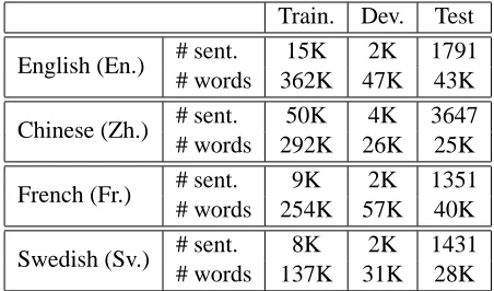
[image:7.612.72.298.57.190.2]Swedish (Sv.) # sent. 8K 2K 1431 # words 137K 31K 28K
Table 1: Training and test data statistics.
Swedish. The data in all these languages is obtained from the CoNLL 2006 shared task on multilingual dependency parsing (Buchholz and Marsi, 2006). We only consider the word and its fine grained POS tag (columns 2 and 5 respectively) and ignore the dependency links in the data. Table 1 shows the data statistics in each of these languages.
We use a second order Hidden Markov Model (Thede and Harper, 1999) based tagger as a baseline tagger in our experiments. This model uses trigram transition and emission probabilities and is shown to achieve good accuracies in English and other lan-guages (Huang et al., 2007). We refer to this as the baseline tagger in the rest of this paper and is used to producen-best list for each candidate sentence. The n-best list for training data is produced using multi-fold cross-validation like Collins and Koo (2005) and Charniak and Johnson (2005). The first block of Table 2 shows the accuracies of the top-ranked tag sequence (according to the Viterbi decoding score) and the oracle accuracies on the 10-best list. As expected the accuracies on English and French are high and are on par with the state-of-the-art systems. From the oracle scores, it is clear that though there is a chance for improvement using reranking, the scope for improvement in English is less compared to the 5 point improvement reported for parsing (Charniak and Johnson, 2005). This indicates the difficulty of the reranking problem for POS tagging in well-resourced languages.
4.1 Reranking Features and Baselines
In this paper, except for Chinese, we use suffixes of length two to four as features in the word view and unigram and bigram tag sequences as features in the
tag view. That is, we convert each word of the sen-tence into suffixes of length two to four and then treat each sentence as a bag of suffixes. Similarly, we treat a candidate POS tag sequence as a bag of unigram and bigram tag features. For Chinese, we use character sequences of length one and two as features for the sentences and use unigram and bi-gram POS tag sequences on the tag view. We did not include any alignment based features, i.e. fea-tures that depend on the position.
We compare our models with a boosting-based discriminative approach (Collins and Koo, 2005) and its regularized version (Huang et al., 2007). In order to enable a fair comparison, we use suffix and tag pairs as features for both these models. For ex-ample, we would generate the following features for the word ‘selling’ in the phrase “the/DT selling/NN pressure/NN”: (ng, NN), (ng, DT NN), (ing,NN), (ing,DT NN), (ling,NN), (ling,DT NN). For com-parison purposes, we also show results by running the baseline rerankers with n-gram features.
4.2 Results
There are following hyper parameters in each of our models, regularization parameterτ, weight parame-terλin the discriminative and softened discrimina-tive models, the linear combination weightw with the Viterbi decoding score, and finally, the size of the lower dimensional subspace (k). We use grid search to tune these parameters based on the devel-opment data set. The optimal hyperparameter values differ based on the model and the language, but the tagging accuracy is relatively robust with respect to these parameter values. For English, the best values for the discriminative model areτ = 0.95,λ= 0.3 andk = 75. For the same language, Fig. 1 shows the performance with respect toτ andλparameters, respectively, with other parameters fixed to their op-timal values. Notice that, although the performance varies it is always more than the accuracy of the baseline tagger (96.74%).
96.74 96.76 96.78 96.8 96.82 96.84 96.86
0.78 0.8 0.82 0.84 0.86 0.88 0.9 0.92 0.94 0.96 0.98 1 Discriminative Softened-Disc Generative
τ
96.74 96.76 96.78 96.8 96.82 96.84 96.86
0 0.1 0.2 0.3 0.4 0.5 0.6 0.7 0.8 Discriminative
Softened-Disc
[image:8.612.87.533.60.237.2]λ
Figure 1: Tagging accuracy with hyperparametersτandλon English development data set.
Development Set Test set
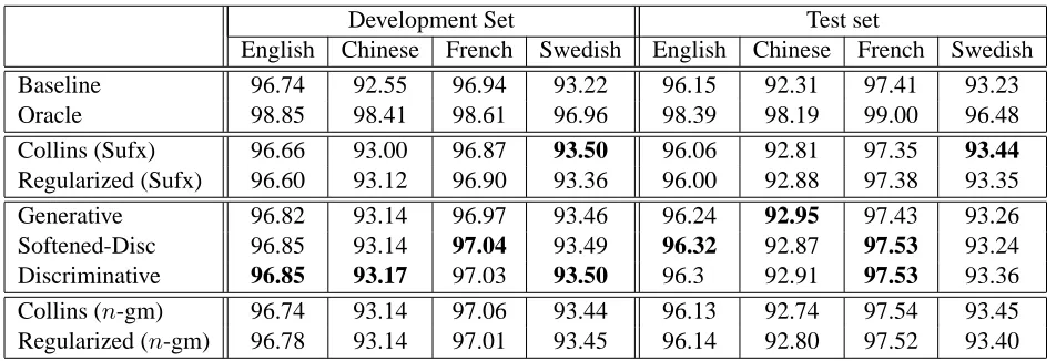
English Chinese French Swedish English Chinese French Swedish Baseline 96.74 92.55 96.94 93.22 96.15 92.31 97.41 93.23 Oracle 98.85 98.41 98.61 96.96 98.39 98.19 99.00 96.48 Collins (Sufx) 96.66 93.00 96.87 93.50 96.06 92.81 97.35 93.44
Regularized (Sufx) 96.60 93.12 96.90 93.36 96.00 92.88 97.38 93.35 Generative 96.82 93.14 96.97 93.46 96.24 92.95 97.43 93.26 Softened-Disc 96.85 93.14 97.04 93.49 96.32 92.87 97.53 93.24 Discriminative 96.85 93.17 97.03 93.50 96.3 92.91 97.53 93.36 Collins (n-gm) 96.74 93.14 97.06 93.44 96.13 92.74 97.54 93.45 Regularized (n-gm) 96.78 93.14 97.01 93.45 96.14 92.80 97.52 93.40
Table 2: Accuracy of the baseline HMM tagger and different reranking approaches. For comparison purposes, we also showed the results of Collins and Koo (2005) its regularized versions withn-gram features. The improvements of our discriminative models are statistically significant atp= 0.01andp= 0.05levels on Chinese and English respectively.
information for Chinese and this additional informa-tion is being exploited by the reranking approaches. Swedish, on the other hand, is a Germanic language with compound word phenomenon which makes the baseline HMM decoder weaker compared to English and French.
The fourth block shows the performance of our models. Except in Swedish, one of our models out-perform the baseline decoder and the other rerank-ing approaches. The fact that our models outperform the baseline system and other reranking approaches indicate that, by considering all the pairwise com-binations of the input features our models capture dependencies that are left by other models. Among the different formulations of our approach,
maxi-mizing the margin between the correct and incorrect candidates performed better than generative, and en-suring that the margin is proportional to the loss of the candidate sequence (discriminative) led to even more improved results. Except in Chinese, our dis-criminative version performed at least as well as the other variants. Compared to the baseline decoder, the discriminative version achieves a maximum im-provement of 0.6 points in Chinese while achieving 0.15, 0.12 and 0.13 points of improvement in En-glish, French and Swedish languages respectively.
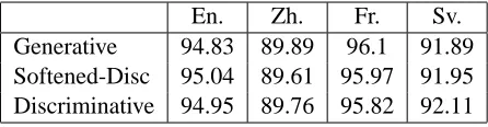
[image:8.612.70.546.273.436.2]En. Zh. Fr. Sv. Generative 94.83 89.89 96.1 91.89 Softened-Disc 95.04 89.61 95.97 91.95 Discriminative 94.95 89.76 95.82 92.11
Table 3: Accuracies without combining with Viterbi de-coding score.
reader should compare our results with the baseline rerankers run with the suffix features. The perfor-mance of these baseline rankers improved when we include the n-gram features but it is still less than the discriminative model in most cases.
Finally, Table 3 shows the performance of our models without combining with the Viterbi decod-ing score. As shown, the performance drops signif-icantly and is in accordance with the behavior ob-served elsewhere (Collins and Koo, 2005).
5 Related Work
In this section, we discuss approaches that are most relevant to our problem and the approach.
In NLP literature, discriminative reranking has been well explored for parsing (Collins and Koo, 2005; Charniak and Johnson, 2005; Shen and Joshi, 2003; McDonald et al., 2005; Johnson and Ural, 2010) and statistical machine translation (Shen et al., 2004; Watanabe et al., 2007; Liang et al., 2006). Collins (2002) proposed two reranking approaches, namely boosting algorithm and a voted perceptron, for the POS tagging task. Later Huang et al. (2007) propose a regularized version of the objective used by Collins (2002) and show an improved perfor-mance for Chinese. In all of the above reranking approaches, the feature functions are defined jointly on the input and output, whereas in our approach, the features are defined separately within each view and the algorithm learns the relationship between them automatically. This is the primary difference between our approach and the existing rerankers.
In principle, our margin formulations are similar to the max margin formulations of CCA (Szedmak et al., 2007) and maximum margin regression (Szed-mak et al., 2006; Wang et al., 2007). These ap-proaches solve the following optimization problem:
min kWk2+C1Tξ (16) s.t. hyi, W φ(x)ii ≥1−ξi ∀i= 1· · ·n
Our approach differs from these formulations in two main ways: the score assigned by our generative model (equivalent to CCA) for an input-output pair (xTi abTyi) can be converted into this format by
substituting W ← baT but in doing so we are ignoring the rank constraint. It is often observed that, dimensionality reduction leads to an improved performance and thus the rank constraint becomes crucial. Another major difference is that, the con-straints in Eq. 16 represent that any input and out-put pair should have at least a margin of 1 (modulo slack), whereas in our approach, the constraints in-clude incorrect outputs along with their loss value. In other words, our formulation is more suitable for the reranking problem while Eq. 16 is more suitable for regression or classification tasks. Our genera-tive model is very similar to the supervised semantic hashing work (Bai et al., 2010) but the way we opti-mize is completely different from theirs.
6 Discussion
In this paper, we proposed a novel family of mod-els for discriminative reranking problem and showed improvements for the POS tagging task in four dif-ferent languages. Here, we restricted our scope to showing the utility of our technique and, hence, did not experiment with different features, though it is an important direction. By using only within space features, our models are able to beat the rerank-ing approaches that use potentially more informa-tive alignment-based features. It is also possible to include alignment-based features into our models by posing the problem as a feature selection problem on the covariance matrices (Jagarlamudi et al., 2011). Our approach involves an inverse computation and an eigenvalue problem. Although our models scale to medium size data sets (our Chinese data set has 50K examples and 33K features), these operations can be expensive. But there are alternative approx-imation techniques that scale well to large data sets (Halko et al., 2009). We leave this for future work.
Acknowledgments
References
Bing Bai, Jason Weston, David Grangier, Ronan Collobert, Kunihiko Sadamasa, Yanjun Qi, Olivier Chapelle, and Kilian Weinberger. 2010. Learning to rank with (a lot of) word features. Inf. Retr., 13(3):291–314, June.
G¨ukhan H. Bakir, Thomas Hofmann, Bernhard Sch¨olkopf, Alexander J. Smola, Ben Taskar, and S. V. N. Vishwanathan. 2007. Predicting Structured Data (Neural Information Processing). The MIT Press.
Peter F. Brown, Vincent J. Della Pietra, Stephen A. Della Pietra, and Robert L. Mercer. 1993. The mathemat-ics of statistical machine translation: parameter esti-mation. Comput. Linguist., 19:263–311, June. Sabine Buchholz and Erwin Marsi. 2006. Conll-x shared
task on multilingual dependency parsing. In Proceed-ings of the Tenth Conference on Computational Nat-ural Language Learning, CoNLL-X ’06, pages 149– 164, Stroudsburg, PA, USA. Association for Compu-tational Linguistics.
Eugene Charniak and Mark Johnson. 2005. Coarse-to-fine n-best parsing and maxent discriminative rerank-ing. In Proceedings of the 43rd Annual Meeting on Association for Computational Linguistics, ACL ’05, pages 173–180, Stroudsburg, PA, USA. Association for Computational Linguistics.
David Chiang, Kevin Knight, and Wei Wang. 2009. 11,001 new features for statistical machine transla-tion. In Proceedings of Human Language Technolo-gies: The 2009 Annual Conference of the North Ameri-can Chapter of the Association for Computational Lin-guistics, NAACL ’09, pages 218–226, Stroudsburg, PA, USA. Association for Computational Linguistics. Michael Collins and Terry Koo. 2005.
Discrimina-tive reranking for natural language parsing. Compu-tational Linguistics, 31:25–70, March.
Michael Collins. 2002. Ranking algorithms for named-entity extraction: boosting and the voted perceptron. In Proceedings of the 40th Annual Meeting on As-sociation for Computational Linguistics, ACL ’02, pages 489–496, Stroudsburg, PA, USA. Association for Computational Linguistics.
Alexander Fraser, Renjing Wang, and Hinrich Sch¨utze. 2009. Rich bitext projection features for parse rerank-ing. In Proceedings of the 12th Conference of the Eu-ropean Chapter of the Association for Computational Linguistics, EACL ’09, pages 282–290, Stroudsburg, PA, USA. Association for Computational Linguistics. Nathan Halko, Per-Gunnar. Martinsson, and A. Joel
Tropp. 2009. Finding structure with randomness: Stochastic algorithms for constructing approximate
matrix decompositions. Technical report, California Institute of Technology.
David R. Hardoon, Sandor R. Szedmak, and John R. Shawe-taylor. 2004. Canonical correlation analy-sis: An overview with application to learning methods. Neural Comput., 16:2639–2664, December.
Harold Hotelling. 1936. Relation between two sets of variables. Biometrica, 28:322–377.
Zhongqiang Huang, Mary Harper, and Wen Wang. 2007. Mandarin part-of-speech tagging and discrim-inative reranking. In Proceedings of the 2007 Joint Conference on Empirical Methods in Natural guage Processing and Computational Natural Lan-guage Learning (EMNLP-CoNLL), pages 1093–1102, Prague, Czech Republic, June. Association for Com-putational Linguistics.
Jagadeesh Jagarlamudi, Raghavendra Udupa, Hal Daum´e III, and Abhijit Bhole. 2011. Improving bilingual projections via sparse covariance matrices. In Proceedings of the 2011 Conference on Empirical Methods in Natural Language Processing, pages 930–940, Edinburgh, Scotland, UK., July. Association for Computational Linguistics.
Mark Johnson and Ahmet Engin Ural. 2010. Rerank-ing the Berkeley and Brown parsers. In Human Lan-guage Technologies: The 2010 Annual Conference of the North American Chapter of the Association for Computational Linguistics, HLT ’10, pages 665–668, Stroudsburg, PA, USA. Association for Computational Linguistics.
Sandra Kubler, Ryan McDonald, Joakim Nivre, and Graeme Hirst. 2009. Dependency Parsing. Morgan and Claypool Publishers.
Percy Liang, Alexandre Bouchard-Cˆot´e, Dan Klein, and Ben Taskar. 2006. An end-to-end discriminative approach to machine translation. In Proceedings of the 21st International Conference on Computa-tional Linguistics and the 44th annual meeting of the Association for Computational Linguistics, ACL-44, pages 761–768, Stroudsburg, PA, USA. Association for Computational Linguistics.
Ryan McDonald, Koby Crammer, and Fernando Pereira. 2005. Online large-margin training of dependency parsers. In Proceedings of the 43rd Annual Meeting on Association for Computational Linguistics, ACL ’05, pages 91–98, Stroudsburg, PA, USA. Association for Computational Linguistics.
Libin Shen, Anoop Sarkar, and Franz Och. 2004. Dis-criminative reranking for machine translation. In Hu-man Language Technology Conference and the 5th Meeting of the North American Association for Com-putational Linguistics: HLT-NAACL 2004, Boston, USA, May.
S. Szedmak, J. Shawe-Taylor, and E. Parado-Hernandez. 2006. Learning via linear operators: Maximum mar-gin regression; multiclass and multiview learning at one-class complexity. Technical report, University of Southampton.
Sandor Szedmak, Tijl De Bie, and David R. Hardoon. 2007. A metamorphosis of canonical correlation anal-ysis into multivariate maximum margin learning. In Proceedings of the fifteenth European Symposium on Artificial Neural Networks.
Ben Taskar, Carlos. Guestrin, and Daphne Koller. 2004. Max margin markov networks. In Proceedings of NIPS 16.
Scott M. Thede and Mary P. Harper. 1999. A second-order Hidden Markov Model for part-of-speech tag-ging. In Proceedings of the Annual Meeting on Asso-ciation for Computational Linguistics, pages 175–182. Association for Computational Linguistics.
Ioannis Tsochantaridis, Thomas Hofmann, Thorsten Joachims, and Yasemin Altun. 2004. Support vec-tor machine learning for interdependent and structured output spaces. In Proceedings of the twenty-first inter-national conference on Machine learning, ICML ’04, pages 104–, New York, NY, USA. ACM.
Zhuoran Wang, John Shawe-Taylor, and Sandor Szed-mak. 2007. Kernel regression based machine trans-lation. In Human Language Technologies 2007: The Conference of the North American Chapter of the As-sociation for Computational Linguistics; Companion Volume, Short Papers, NAACL-Short ’07, pages 185– 188, Stroudsburg, PA, USA. Association for Compu-tational Linguistics.