Comparison of Three Different Cardiac T2-Mapping
Techniques at 1.5 Tesla
Suliman S Hashemi
1, Ruud van Heeswijk
2, Janine Schwitter
3, Roger Hullin
4, Matthias Stube
2,5and Juerg
Schwitter*
61Cardiovascular Department, Cardiac Surgery, University Hospital Lausanne, CHUV, Switzerland
2Center of Biomedical Imaging, Federal Institute of Technology (EPFL) and University Hospital Lausanne, CHUV, Switzerland
3University of Fribourg, Medical School, Fribourg, Switzerland
4Cardiovascular Department, Cardiology, University Hospital Lausanne, CHUV, Switzerland
5Department of Radiology, University Hospital Lausanne, CHUV, Switzerland
6Cardiac MR Center of the University Hospital Lausanne (CRMC), CHUV, Switzerland
Received: February 10, 2018; Published: March 21, 2018
*Corresponding author: Juerg Schwitter, Centre de la RM Cardiaque du CHUV, Centre Hospitalier Universitaire Vaudois (CHUV), Lausanne, Switzerland,
Tel: ; Email:
ISSN: 2574-1241
Biomed J Sci & Tech Res
Introduction
For the detection of inflammatory myocardial diseases [1] and the characterization of myocardial edema in the setting of ischemic heart disease, CMR techniques, and in particular, novel T2-mapping
techniques, gain increasing acceptance. While T2-weighted imaging strategies allow for the detection of myocardial edema, T2-mapping techniques are considered advantageous as they yield quantitative
Research Article Open Access
Abstract
Background: T2-mapping techniques gain increasing acceptance to study myocardial edema in inflammatory and ischemic heart diseases. Study Aim: To compare the performance of a breath-hold and two free-breathing T2-mapping techniques in a prospective design in healthy subjects.
Methods: Three different sequences for T2-mapping were tested on a clinical CMR scanner (Aera, Siemens, Germany) at 1.5T: a) Breath-hold 2D-acquisition technique (2D-BH)
b) Free-breathing 2D-technique applying a diaphragmatic navigator (2D-FBNav), and
c) Free-breathing 3D-technique applying self-navigation for respiratory motion correction (3D-FBSN). T2-values were quantified
in 6 segments per short-axis slice on 5 slices (2D-BH and 3D-FBSN) and 3 slices (2D-FBNav) covering the left ventricle. Analyses were also
performed with larger segments (8- and 2-segment models). As a quality measure, the coefficient of variation (CV%=standard deviation of
T2-value expressed as percentage of mean T2) was determined. Contours were drawn manually by 2 observers using commercial software (Gyrotools, Zurich, Switzerland). T2 differences between techniques, slices, and segments were evaluated by repeated-measures ANOVA and post-hoc Bonferroni-correction.
Results: With 2D-BH, diagnostic images were obtained in all 13 volunteers (=390 segments). With 2D-FBNav 3 slices/volunteer were
acquired and quality was non-diagnostic in 5 slices yielding 204 segments for analysis. With 3D-FBSN 1 volunteer was not evaluable yielding
360 segments for analysis. Mean T2-values (=T2 averaged over all segments) were higher for the 3D-FBSN (54.4±5.4ms vs. 48.5±2.4ms and 45.9±4.4ms for 2D-BH and 2D-FBNav, respectively, p<0.002). The CV% of the 3D-FBSN technique was higher vs. both, 2D-BH and 2D-FBNav
(12.1±5.4% vs. 7.0±1.1% and 8.3±3.9%, respectively, p<0.02).
Conclusion: At 1.5T, most reliable T2 results with a low coefficient of variation were obtained by the 2D-BH technique. The 2D-FBNav technique is considered as an alternative if breath-holding capacity is not sufficient. The 3D-FBSN technique is not at the same level of
measures of T2 and this should allow for more reliable inter-subject comparisons, e.g. for follow-up studies to evaluate treatment response. The quantitative T2 mapping strategy should also facilitate multicenter trials and inter-study comparisons. However, T2 mapping pulse sequences are demanding as they require 3 or more image acquisitions (with different T2-waiting times) to reconstruct the T2-map. Breath-hold approaches are proposed to generate T2 maps [2] but some compromises are unavoidable regarding spatial resolution and/or acquisition window duration in order to fit the acquisition into a single breath-hold.
Alternatively, free-breathing strategies could be superior with regard to spatial resolution and acquisition window duration, if breathing motion can be adequately corrected for [3,4]. For such breathing motion correction, navigators applied to the right hemidiaphragm were used [3] or self-navigation strategies [4]. The aim of this study was to evaluate the performance of 3 different T2-mapping techniques, i.e.
a) A breath-hold 2D acquisition technique (2D-BH)
b) A free-breathing 2D acquisition technique applying a diaphragmatic navigator approach (2D-FBnav)
c) A free-breathing 3D acquisition technique applying self-navigation for breathing motion correction (3D-FBSN). As most clinical CMR studies are performed on 1.5T systems [5], both the2D-FBnav and 3D-FBSN pulses sequences developed for 3T [3,4] were transferred onto a 1.5T system for this comparative study.
Methods
Volunteers: The study enrolled 13 healthy subjects (5 men, 8 women, age 24-47 years old). Exclusion criteria were presence of any cardiac pathology, a history of cardiac interventions, any past or current cardiac medication, and presence of a pacemaker/ defibrillator. The study protocol was approved by the local Ethics Committee and all study subjects gave written informed consent before study participation.
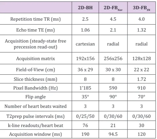
T2 Mapping Pulse Sequences: In each subject, 3 different cardiac T2 mapping pulse sequences were acquired at 1.5T (Magnetom Area, Siemens Healthcare, Germany) in a single scanning session starting with a 2D breath-hold acquisition (2D-BH) [2], followed by a high spatial resolution free-breathing 2D acquisition (2D-FBNav) [3], and ending with a high spatial resolution free-breathing self-navigation 3D acquisition (3D-FBSN) [4], Table 1. With the 2D-BH, 5 short-axis slices of the left ventricle (LV) were acquired distributed evenly along the long axis of the LV. With the 2D-FBNav sequence, only 3 LV short-axis slices were acquired (avoiding the most basal and most apical short-axis slice) to account for the longer acquisition duration for this sequence. Finally, with the 3D-FBSN sequence the entire LV was covered. Table 1: Magnetic resonance imaging parameters for the 3 different techniques
2D-BH 2D-FBNav 3D-FBSN
Repetition time TR (ms) 2.5 4.5 4.0
Echo time TE (ms) 1.06 2.1 1.32
Acquisition (steady-state free
precession read-out) cartesian radial radial
Acquisition matrix 192x156 256x256 128x128
Field-of-View (cm) 36 x 29 30 x 30 22 x 22
Slice thickness (mm) 8 8 1.72
Pixel Bandwidth (Hz) 1’185 590 910
Flip angle 35° 90° 70°
Number of heart beats waited 3 3 3
T2prep pulse intervals (ms) 0/25/50 0/30/60 0/30/60
k-line readouts/heart beat 76 21 30
Acquisition window (ms) 190 94.5 120
This table shows the MRI pulse sequence parameters for the three different techniques.
Figure 1: T2-mapping images in the 3 different techniques. Examples of a mid-ventricular short-axis T2 map obtained with 2D-BH (A), 2D-FBNav (B), and 3D-FBSN (C). Reference point (cross) is the anterior insertion point of the right ventricle at the septum. Blue/red: epicardial/endocardial contours.
Data Analysis: For the 2D-BH and 2D-FBNav acquisitions, on each slice, the epicardial and endocardial contours of the LV myocardium were manually drawn with a thickness of 3 mm, approximately 1.5 mm from each side of the middle line of the
on the LV (Figure 1) yielding 30 and 18 segment models for the 2D-BH and 2D-FBNav acquisitions, respectively. For the analysis of the 3D-FBSN acquisition, 5 short-axis slices were selected out of the 3D volume based on anatomical landmarks (Figure 1) to match the short-axis slices of the 2D acquisitions (yielding 30 segments per
heart for this analysis). Analyses were performed using commercial software (Gyrotools GmbH, version 2.2.1, Zurich, Switzerland). To fully exploit the LV coverage by the 3D-FBSN acquisition, the heart was divided into larger segments yielding one 8-segment and three 2-segments models as shown in Figure 2.
Figure 2: Heart division in the different segment-division models. The whole heart analysis yields one 8-segment model (antero-lateral (1;5), infero-lateral (2;6), infero-septal (4;8), and antero-septal (3;7) for the basal and midventricular level, respectively) as well as three 2-segment models dividing the heart into an anterior and inferior half (segments 1;3;5;7 and 2;4;6;8, respectively), a lateral and septal half (segments 1;2;5;6 and 3;4;7;8, respectively), and a basal and mid-ventricular half (segments 1;2;3;4 and 5;6;7;8, respectively). For these analyses the apex was excluded to minimize partial volume artifacts.
To compare these data with the 2D data sets, several segments and slices of the 2D data were combined to match these 8- and 2-segments models. For 2D-BH, e.g., the basal segments i.e. segments 1-4 on (Figure 2) were calculated by averaging slice 1, slice 2, and half of slice 3 and the mid segments i.e. segments 5-8 on (Figure 2) by averaging half of slice 3, and the entire slice 4 and slice 5. For 2D-FBNav the basal and mid segments were calculated by averaging basal slice 1 and half of slice 2 and by averaging half of slice 2 and slice 3, respectively. In analogy, segments of a slice were combined to match the 8-segment and 2-segment models. The pulse sequences used in this study are all well validated against known T2 values determined in phantoms [3,4,7].
As the true myocardial T2 in humans is difficult to obtain, we used the variability of T2 values measured in the volunteer group as an indicator of data quality. This variability is expected to be small for a robust measurement when performed in a homogenous group
of healthy volunteers. Measurement variability was expressed for each segment (of the 30-segment, 18-segment, 8-segment and the three 2-segment models obtained in the 13 volunteers) as the SD (for each segment) divided by the mean T2 value for this segment, i.e. by the coefficient of variation (CV% = SD expressed as percentage of the mean T2 value).
Statistics
Continuous data are presented as mean ± standard deviation. T2 values and CV% for the 3 pulse sequences were compared by 1-one way ANOVA for repeated measures with post-hoc Bonferroni correction. CV% for the 3 techniques was compared on the basis of the 18 segment model (3 slices with 6 segments each). CV% was also compared between the 18-segment, the 8-segment, and the three 2-segment models for each pulse sequence. A post-hoc corrected p value <0.05 was considered significant.
Results
Comparison of 2D-BH, 2D-FBNav, and 3D-FBSN
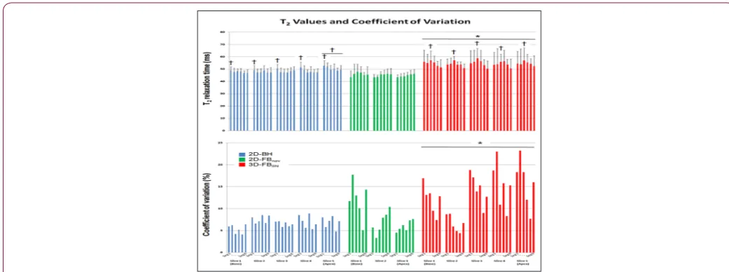
In all volunteers the 2D-BH T2 mapping sequences yielded complete data sets of diagnostic quality. With the 2D-FBNav sequence (with 3 slices per subject) 1 slice was of non-diagnostic quality in 3 subjects each, and in 2 additional subjects, slice 3 was not acquired (as the irregular breathing pattern did not allow finishing the acquisition in time). For the 3D-FBSN pulse sequence, data of one subject were not correctly acquired (due to inaccurate tracking of the heart silhouette). The T2 values, averaged over all segments, for 2D-BH and for 2D-FBNav were 48.5±2.4ms and 45.9±4.4ms, respectively, which were lower than 54.4±5.4ms measured by 3D-FBSN (p<0.002 for both, no difference for 2D-BH vs. 2D-FBNav, Figure 3A). The CV% of the 3D-FBSN technique was higher vs both, the 2D-BH and 2D-FBNav acquisition (CV% 12.1±5.4% vs 7.0±1.1% and vs 8.3±3.9%, respectively, p<0.02 for both, Figure 3B).
Distribution of T2 Values in Normal Myocardium for the
three T2 Mapping Techniques
With 2D-BH, T2 of 50.4±2.9ms in slice 5 was slightly higher than in the other 4 slices (47.7±2.0ms, 47.8±3.1ms, 47.7±2.0ms, 48.3±2.9ms, respectively, p<0.001). Also, the T2 of the anterior segment was higher than the T2 of the other segments (50.5±3.2ms
vs segments 2, 3, 4, 5, and 6 with 48.8±2.6ms, 47.9±2.6ms, 48.4±3.1ms, 47.6±2.0ms, and 48.0±2.7ms, respectively, p<0.005). Inspection of Figure 3A indicates that slice 5 contributes most to the elevated T2 in the anterior segment. For 2D-FBNav, no differences in T2 were found between slices or segments. For 3D-FBSN, no differences in T2 between slices were found. However, T2 in the infero-lateral segment 3 was higher in comparison to the “opposite” antero-septal segment 6 (57.2±6.7ms vs 51.1±6.4ms, p<0.003; Figure 3A).
Influence of Size of Myocardial Segments on Robustness
of T2 Measurements
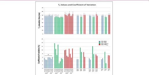
For the models with larger segment sizes, T2 did not differ for the 3 techniques (Figure 4A). For 3D-FBSN, CV% showed a trend to diminish with increasing sizes of segments (CV% for 18-, 8-segment, and 2-segment models: 12.1±5.4%, 8.6±2.1%, 7.2±0.6%, and 7.6±1.9%, and 7.1±0.1%, respectively, ns, Figure 4B). Similarly, for 2D-FBnav, there was a trend of CV% to decrease with increasing segment size (CV% for 18-, 8-, and 2-segment models: 8.3±3.9%, 5.5±0.6%, 6.0±2.0%, 5.7±0.7%, and 6.1±0.1%, respectively, ns, Figure 4B). For the 2D-BH data, the models with 8 and 2 segments yielded slightly lower CV% vs. the 18-segment model (5.6±0.6%, 5.0±0.1%, 5.1±0.5%, 5.2±0.4% vs 7.0±1.1%, respectively p<0.001, Figure 4B).
Figure 4: Segmental T2 (A) and CV% (B) values for the three T2-mapping sequences for models with 8 and 2 segments per heart. For models with larger segments, CV% tended to decrease with 2D-FBNav 3D FBSN, which reached statistical significance for 2D-BH (*significant vs 18-segment model; for details, see results section).
Discussion
For both, the 2D-BH and the 2D-FBNav technique, very similar T2 values were obtained with 48.5±2.4ms and 45.9±4.4ms, respectively. Also, these T2 values were homogeneously distributed in the 18 segments per heart as shown in Figure 3A. For the 2D-FBNav technique, T2 values were not different over the 3 short-axis slices or in the different segments. For the 2D-BH technique, the
in the apical slice is a partial volume artifact in the apical region. With the 3D-FBSN technique, higher T2 values were obtained in comparison with the other two techniques. This T2 elevation was most prominent in the infero-lateral segment, where T2 was higher than in the “opposite” antero-septal segment (Figure 3A).
This may be explained by the fact that the infero-lateral segment is more distant from the surface coil than the antero-septal segment causing a reduced signal-to-noise ratio (SNR) in this infero-lateral segment. A slight T2 overestimation in regions with lower SNR has been shown for 3D-FBSN at 3T [4,8]. Regarding the robustness of the three acquisition strategies, the 2D-BH technique proved to be very reliable. In all subjects, the 2D-BH technique yielded analyzable data and the CV% was small with 7.0±1.1%. As shown in Figure 3B, the CV% is also acceptably small for 2D-FBNav with 8.3±3.9%. However, 5 out of 39 short-axis slices were not evaluable with 2D-FBNav, i.e. data were diagnostic in only 87%, and navigator gating is typically related to longer acquisitions. Nevertheless, in case of inadequate breath-holding capabilities, the 2D-FBNav sequence can be considered as an alternative for T2 mapping.
Unlike 2D-BH and 2D-FBNav, the 3D-FBSN technique is associated with significantly larger CV% of 12.1±5.4% and as a consequence, this self-navigated T2 mapping technique in its current form loses too much SNR in the transition from 3T to 1.5T, and would require further refinement before it can be recommended for clinical application. One might argue, that
analyzing only 5 slices out of a 3D volume (as acquired with this 3D-FBSN sequence), would not adequately exploit the full 3D-FBSN performance. While the CV% of the 3D-FBSN technique tended to improve with larger segments (from 12.1±5.4% for 18 segments to 7.1±0.1% for 2 segments), it was not superior in comparison to the 2D-BH technique even when compared with small segments (CV% of 7.0±1.1% for the 18-segment model).
In recent publications, T2 values of healthy volunteers were reported as shown in Figure 5 using a breath-hold T2prep BSSFP technique [2,9-12] (corresponding to 2D-BH used in the current study) or a gradient-echo (echo-planar) multi-echo spin-echo technique (GraSE technique) either applied during a breath-hold [12-14] or combined with navigators for free breathing [12,15]. As shown in Figure 5, which summarizes these findings, normal T2 values measured by the different techniques were similar, ranging from 52.2ms to 58.6ms [2,9-15], while the T2 normal value for the current 2D-BH approach was 48.5ms. When comparing the variability of the T2 measurements, the current 2D-BH technique with a CV% of 4.9% compares well with the CV% reported in the literature ranging from 3.7% to 6.8% [2,9-15], while the variability of the tested 2D-FBNav and 3D-FBSN are considerably higher with 9.6% and 9.9%, respectively. This translates in an upper limit of normal T2 values for the 2D-BH technique of 53.3ms which is lower than reported previously ranging from 57.3ms to 60.1ms using the same T2prep BSSFP technique [2,9-12].
Figure 5: Mean T2 values measured with 2D-BH, 2D-FBNav, and 3D-FBSN versus mean T2 values from the literature (2,9-15). For 2D-BH, T2 tends to be smaller in comparison to published T2 (Figure 5a), while variability, i.e. CV%, is comparable to other 2D breath-hold techniques reported in the literature (Figure 5b). For the free-breathing 2D-FBNav and 3D-FBSN, CV% is substantially higher versus published data. Gra SE: gradient-echo (echo-planar) multi-echo spin-echo technique; other abbreviations as mentioned in the text.
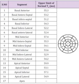
The segmental normal values of the 2D-BH approach for the 17-segment model are given in Table 2. In our study the ROI’s for T2 determination were drawn strictly avoiding signals from blood pool or epicardial fat, which was achieved by restricting the ROI to a width of 3 mm. This may have contributed to the low variability of data even when T2 values were assessed in small segments allowing T2 quantification in 30 segments per heart. The fact, that sequence performances were assessed in healthy volunteers
Figure 6: Example: Acute ST elevation myocardial infarction. 50-years old diabetic patient with anterior STEMI, investigated by CMR 5 days after percutaneous coronary intervention of the left anterior descending coronary artery. Cine acquisitions demonstrate severe hypokinesia of the anterior and septal walls with global LV ejection fraction of 45%, mild pericardial effusion, and increased LV mass of 103g/m2 (normal <78g/m2) probably due to myocardial edema (LVEDV: 83ml/m2). The bull’s eyes show distribution of necrosis (with microvascular obstruction) and of myocardial edema quantified by T2 mapping. Distribution of late gadolinium enhancement (LGE) can also be quantitated by T1 mapping before and after contrast medium administration. The T2 mapping bull’s eye shown in Figures 6-8 uses the threshold values for elevated T2 as presented in Table 2.
Figure 7: Example: Acute myocarditis. 44-year old female patient with complete AV block and chest discomfort, no elevation of troponines. The CMR examination reveals extensive myocardial edema by elevated T2 values, see also bulls eye. A non-quantitative STIR image demonstrates increased signal in concordance with the T2 mapping images (red arrows). Minimal necrosis in the basal infero-septal segment (orange arrow) is detected by late gadolinium enhancement (LGE), while the edematous hypokinetic anterior wall (red arrows on SSFP images) is free of necrosis. Enhancement of the pericardium (white arrows) is compatible with mild pericarditis. Endomyocardial biopsies confirm lymphocytic infiltrates, i.e. myocarditis. Follow-up CMR 4 months later confirms complete resolution of myocardial edema in all LV segments. White arrows on the follow-up T2 maps indicate artifacts due to an electrode in the RV of an MR-conditional ICD.
Table 2: Upper limit of normal for T2 values of the 2D-BH technique - 17-Segment Model.
S.NO Segment Normal TUpper limit of 2 (ms)
1 Basal Anterior 55.3
2 Basal Antero-Septal 53.2
3 Basal infero-septal 51.2
4 Basal Inferior 54.3
5 Basal Infero-Lateral 52.2
6 Basal antero-lateral 52.4
7 Mid Anterior 57.4
8 Mid Antero-Septal 55.3
9 Mid Infero-Septal 54.1
10 Mid Inferior 53.6
11 Mid Infero-Lateral 52.9
12 Mid Antero-Lateral 54.2
13 Apical Anterior 59.9
14 Apical Septal 53.1
15 Apical Inferior 57.1
16 Apical Lateral 54.9
17 Apex
--Upper limit of normal is upper 95%-confidence limit. The normal values of the 16 segments were calculated as follows: Values of slice 3 (=mid-ventricular slice) yielded values for segments 7 to 12. Averaging slice 1 and 2 (basal slices) yielded values for segments 1 to 6 and averaging slice 4 and 5 yielded values for segments 13 to 16. For the apical slice, segment 14 was the mean of the 2 septal segments of slice 4 and 5, segment 16 was the mean of the 2 lateral segments of slice 4 and 5.
Conclusion
Most reliable T2 results with a low coefficient of variation were obtained by the 2D-BH technique. The 2D-FBNav technique is considered as an alternative if breath-holding capacity is not sufficient. The 3D-FBSN technique is not at the same level of robustness as the breath-holding techniques and further refinement is needed before it can be considered an alternative for clinical application.
Acknowledgment
Supported by grants from the Swiss Heart Foundation and the Swiss National Science Foundation (PZ00P3-154719) to RB vH and the Swiss National Science Foundation (310030_163050 / 1) to JS
References
1. Caforio ALP, Pankuweit S, Arbustini E (2013) Current state of knowledge on aetiology, diagnosis, management, and therapy of myocarditis: a
position statement of the European Society of Cardiology Working Group on Myocardial and Pericardial Diseases. Eur Heart J 34(33): 2648a-2648d.
2. Giri S, Chung YC, Merchant A (2009) T2 quantification for improved
detection of myocardial edema. J Cardiovasc Magn Reson 11: 56.
3. Van Heeswijk R, Feliciano H, Bongard C (2012) Free-Breathing Magnetic Resonance T2-mapping of the Heart for Longitudinal Studies at 3T. JACC
CV Imaging 5(12): 1231-1239.
4. Van Heeswijk R, Piccini D, Feliciano H, Hullin R, Schwitter J, et al. (2015) Self-navigated isotropic three-dimensional cardiac T2 mapping. Magn
Reson Med 73(4): 1549-1554.
5. Bruder O, Wagner A, Lombardi M (2013) European Cardiovascular Magnetic Resonance (EuroCMR) registry--multi national results from
57 centers in 15 countries. J Cardiovasc Magn Reson 15: 1-9.
6. Cerqueira MD, Weissman NJ, Dilsizian V, Jacobs AK, et al. (2002) Standardized myocardial segmentation and nomenclature for tomographic imaging of the heart. A statement for healthcare professionals from the Cardiac Imaging Committee of the Council on Clinical Cardiology of the American Heart Association. Circulation
105(4): 539-542.
7. Giri S, Shah S, Xue H (2012) Myocardial T (2) mapping with respiratory navigator and automatic nonrigid motion correction. Magn Reson Med 68(5): 1570-1578.
8. Bano W, Feliciano H, Coristine AJ, Stuber M, van Heeswijk RB (2017) On the accuracy and precision of cardiac magnetic resonance T2 mapping:
A high-resolution radial study using adiabatic T2 preparation at 3 T. Magn Reson Med 77(1): 159-169.
9. Verhaert D, Thavendiranathan P, Giri S (2011) Direct T2 Quantification
of Myocardial Edema in Acute Ischemic Injury. JACC Cardiovascular
Imaging 4(3): 269-278.
10. Thavendiranathan P, Walls M, Giri S, Verhaert D, Rajagopalan S, et al. (2012) Improved detection of myocardial involvement in acute
inflammatory cardiomyopathies using T2 mapping. Circ Cardiovasc
Imaging 5(1): 102-110.
11. Miller CA, Naish JH, Shaw SM (2014) Multiparametric cardiovascular magnetic resonance surveillance of acute cardiac allograft rejection and characterisation of transplantation-associated myocardial injury: a pilot study. J Cardiovasc Magn Reson 16: 52.
12. Baeßler B, Schaarschmidt F, Stehning C (2016) Reproducibility of three different cardiac T2-mapping sequences at 1.5T. J Magn Reson Imaging 44(5): 1168-1178.
13. Bohnen S, Radunski UK, Lund GK (2017) Tissue characterization by T1 and T2 mapping cardiovascular magnetic resonance imaging to monitor
myocardial inflammation in healing myocarditis. Eur Heart J - CVI
18(17): 744-751.
14. Luetkens JA, Homsi R, Sprinkart AM (2016) Incremental value of quantitative CMR including parametric mapping for the diagnosis of acute myocarditis. Eur Heart J Cardiovascular Imaging 17(2): 154-161.
15. Bönner F, Janzarik N, Jacoby C (2015) Myocardial T2 mapping reveals age- and sex-related differences in volunteers. J Cardiovasc Magn Reson
Submission Link: https://biomedres.us/submit-manuscript.php
Assets of Publishing with us
• Global archiving of articles
• Immediate, unrestricted online access • Rigorous Peer Review Process • Authors Retain Copyrights • Unique DOI for all articles
https://biomedres.us/