Scholarship@Western
Scholarship@Western
Electronic Thesis and Dissertation Repository
8-26-2013 12:00 AM
Modelling Credit Value Adjustment Using Defaultable Options
Modelling Credit Value Adjustment Using Defaultable Options
Approach
Approach
Sidita Zhabjaku
The University of Western Ontario
Supervisor Matt Davison
The University of Western Ontario
Graduate Program in Statistics and Actuarial Sciences
A thesis submitted in partial fulfillment of the requirements for the degree in Master of Science © Sidita Zhabjaku 2013
Follow this and additional works at: https://ir.lib.uwo.ca/etd
Part of the Statistical Models Commons
Recommended Citation Recommended Citation
Zhabjaku, Sidita, "Modelling Credit Value Adjustment Using Defaultable Options Approach" (2013). Electronic Thesis and Dissertation Repository. 1503.
https://ir.lib.uwo.ca/etd/1503
This Dissertation/Thesis is brought to you for free and open access by Scholarship@Western. It has been accepted for inclusion in Electronic Thesis and Dissertation Repository by an authorized administrator of
MODELLING CREDIT VALUE ADJUSTMENT USING DEFAULTABLE
OPTIONS APPROACH
(Thesis format: Monograph)
by
Sidita Zhabjaku
Graduate Program in Statistics and Actuarial Science
A thesis submitted in partial fulfillment
of the requirements for the degree of
Master of Science
The School of Graduate and Postdoctoral Studies
The University of Western Ontario
London, Ontario, Canada
c
This thesis calculates Credit Value Adjustment on defaultable options. The prices of
default-able European options are computed through analytical, quadrature approximation and Monte
Carlo simulations under the assumption of a constant rate of default. Subsequently, we propose
to inversely relate the company’s instantaneous rate of default to its underlying stock price,
re-sulting in a non-constant rate of default. This allows for a new approach to estimate the default
of company different from previous work where default is calculated through historical data. The rationale behind this idea relies on the fact that price of the stock plunges before the event
of default. For a given set of option parameters, we show that it is possible to find an optimal
intensity, which produces the same prices of European options under a simpler framework.
However, this intensity fluctuates with changes in other parameters. Implementation details
and analysis of the results are provided.
Keywords: Defaultable Options, Credit Value Adjustment, Poisson Process
Acknowledgements
I would like to take this opportunity and say thank you to my supervisor Dr. Matt Davison for
his guidance, encouragement and undivided support through out my Masters program. Without
his useful comments, remarks and infinite patience this thesis would not have been completed.
I would also like to thank all faculty, staffand graduate students in the department of Ac-tuarial & Statistical Science for always being helpful and kind. A special thanks goes to my
office mates for making the office like my second home.
To my sister Besmira for always encouraging me and teaching me that anything is possible
and to Kyle, for always believing in me and giving me his unconditional support throughout all
my years at Western.
Last but not least, I would like to express my deepest appreciation to my loving parents,
Myfit and Rudina, who always sacrificed everything for my happiness. Without their love none
of this would have been possible.
Contents
Abstract ii
Acknowledgements iii
List of Figures viii
List of Appendices xii
1 Introduction and Motivation 1
1.1 Introduction to Credit Value Adjustment . . . 1
1.2 Background on CVA and its Change from Basel II to III . . . 3
1.3 Thesis at a Glance . . . 7
2 Background Review 9 2.1 Counterparty Credit Risk . . . 9
2.2 CVA Equation . . . 9
2.3 CVA Calculations in the Literature . . . 12
2.4 Black-Scholes Equation . . . 15
2.5 Structural Models . . . 18
2.5.1 Merton Model . . . 18
2.5.2 Black Cox Model . . . 19
2.6 Reduced Form Models . . . 20
2.7 Conclusion . . . 20
3 Detailed Analysis of Constant Default Rate Case 22 3.1 Introduction to Constant Default Arrivals . . . 22
3.2 Homogeneous Poisson Processes . . . 23
3.4 Analytical Approximation for Defaultable Option Prices . . . 28
3.4.1 Taylor Series Approximation Method for Standard Normal . . . 30
3.4.2 Discretization of Taylor Series Approximation, Second Term . . . 33
3.4.3 Discretization of Taylor Series Approximation, Third Term . . . 36
3.5 Problems with Taylor Series Approximation and Errors . . . 38
3.6 Quadrature Solution to Defaultable Option with Constant Default Arrival . . . . 41
3.6.1 Risk Free Interest Rate of Zero . . . 41
3.6.2 Non Zero Risk Free Interest Rate . . . 42
3.7 Conclusion . . . 43
4 Pricing Results for Variable Default Rate Case 45 4.1 Non-Constant Default Rates . . . 45
4.1.1 Inhomogeneous Poisson Process . . . 45
4.2 Constant and Non-Constant Default Rates . . . 47
4.2.1 Method 1 . . . 48
4.2.2 Method 2 . . . 50
4.2.3 Method 1 Results . . . 52
4.2.4 Method 2 Results . . . 53
4.3 Model Validation . . . 54
4.4 Non-Constant Default Against Constant Results and Comparison . . . 61
4.5 Credit Value Adjustment . . . 72
4.6 Conclusion . . . 76
5 Conclusion 79 5.1 Discussion . . . 79
5.2 Financial Modelling Implications . . . 80
5.3 Future Work . . . 81
References 83
A Basel Committee on Banking Supervision Countries 86
B Detailed Analytic Calculations for Defaultable Options 87
C Monte Carlo Simulations with Errors 92
Curriculum Vitae 100
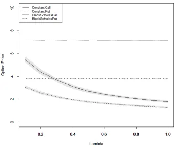
3.1 Defaultable call and put option prices against Black-Scholes option prices with
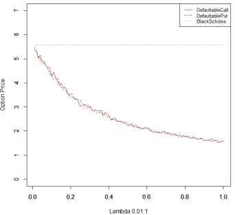
r=2%,S = K =$35,R=70%,σ= 18%,T =5, with a 99% confidence level. 27 3.2 Defaultable call and put option prices withr = 0%,S = K = $35, σ = 18%,
R= 70%,T = 5, for error bars of the simulations refer to Appendix C, Figure C.1. . . 28
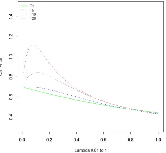
3.3 Analytical approximation of equation (3.30) with different maturity dates, T=1, 5, 10, 20,σ =18%,r= 0%,R= 70% andS = K =$35. . . 34 3.4 Analytical approximation of equation (3.36) using second term Taylor
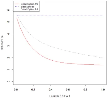
expan-sion. Parameters: S0 = K =$35, σ=18%,r =0%,T =5,R=70%,n=1000. 36 3.5 Analytical approximation with the second and third term of the Taylor Series,
comparing it to Black-Scholes. Parameters:S0 =K =$35,σ= 18%,r= 0%,
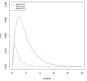
T =5,R=70%,n= 1000. . . 38 3.6 Errors of the first three terms of the Taylor expansion withλfrom 0.01 to 10. . 40
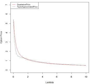
3.7 Comparison between a quadrature solution of equations (3.51) added with (3.52)
and the analytical solution that we derived in Section 3.4, withλfrom 0.01 to
10,σ=18%,r= 0%,T =5,R=70%,S = K =$35. . . 42 3.8 Comparison between quadrature and simulated results, withλfrom 0.01 to 10,
r=2%,σ =18%,R=70%,S = K= $35 andT =5. . . 43
4.1 Method 1 comparison between constant and non-constant default rates of a call
and put option, through Monte Carlo simulations, withCfrom 5 to 50,r= 2%, σ=18%,S = K =$35,R=70% andT =5. For error bars of the options and default times refer to Appendix C, Figure C.2, and Figure C.3. . . 53
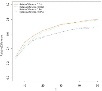
4.2 Method 1 relative difference between constant and non-constant default rates of a call and put option with the Black-Scholes pricing of such options, with
parametersC from 5 to 50, r = 2%, σ = 18%, S = K = $35, R = 70% and
T =5. . . 54 4.3 Method 2 results on the comparison between constant and non-constant default
rates of a call and put option, through Monte Carlo simulations, withCfrom 5
to 50,r= 2%,σ=18%,S = K =$35,R=70% andT =5. . . 55 4.4 Method 2 results on the comparison of relative difference between constant
and non-constant default rates of a call and put option with the Black-Scholes
pricing of a call and put, with parametersC from 5 to 50, r = 2%, σ = 18%,
S =K = $35,R= 70% andT = 5. . . 56 4.5 Comparison of formula (4.24) with parametersC from 5 to 50, r = 2%, σ =
18%,S = K =$35 andT = 5. . . 57 4.6 Survival probability with the constant and non-constant default rate with
pa-rametersCfrom 5 to 50,r= 2%,σ =18%,S = K = $35 andT = 5. For error bars refer to Appendix C, Figure C.4. . . 58
4.7 Survival probability with the constant and non-constant default rate with
pa-rametersC from 5 to 50,r = 2%, σ = 35%, S = K = $35 and T = 5, with error bars at a 99% confidence level. . . 59
4.8 Put-Call Parity check holds for the defaultable options with C from 5 to 50,
r=2%,σ =35%,S =K = $35,R= 70% andT =5. . . 60 4.9 Comparison of default and non default option pricing with a range of different
strike prices denoted by K, where C = 15, r = 2%, σ = 18%, S = $35,
R=70% andT =5. . . 62 4.10 Comparison of constant default and non-constant default rate option pricing
with a range of different C values, where R = 100%, r = 2%, σ = 18%,
S =K = $35 andT = 5. For the error bars refer to Appendix C, Figure C.5. . . 63 4.11 Comparison of default and non default option pricing with a range of different
C values, whereR=0%,r= 2%,σ=18%,S = K =$35 andT =5. . . 64
C, R = 70%, r = 2%, S = K = $35 andT = 5. For the error bars refer to Appendix C, Figure C.6. . . 65
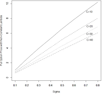
4.13 Put option pricing with non-constant default rate, at different values ofσand
C, R = 70%, r = 2%, S = K = $35 andT = 5. For the error bars refer to Appendix C, Figure C.7. . . 66
4.14 Call option pricing with constant default rate, at different values ofσ andC,
R=70%,r= 2%,S = K =$35 andT = 5. . . 67 4.15 Put option pricing with constant default rate, at different values of σ and C,
R=70%,r= 2%,S = K =$35 andT = 5. . . 68 4.16 Absolute difference of call option pricing with constant and non-constant
de-fault rates, at different values ofσandC,R= 70%,r= 2%,S =K = $35 and
T =5. . . 69 4.17 Absolute difference of put option pricing with constant and non-constant
de-fault rates, at different values ofσandC,R= 70%,r= 2%,S =K = $35 and
T =5. . . 70 4.18 Comparison of the average default rate given in equation 4.28 and the
non-constant default rate calculated through Monte Carlo Simulations, shown at
different values ofσs whereC= 30,R=70%,r= 2%,S = K =$35 andT = 5. 71 4.19 Comparison of the average default rate, ¯λ∗called the newλ, given in equation
4.32 and the non-constant default rate calculated through Monte Carlo
Simu-lations, shown at different values of σs whereC = 30, R = 70%, r = 2%,
S =K = $35 andT = 5. . . 72 4.20 Call option pricing with constant default rate, ¯λ∗, at different values ofσs where
R = 70%, r = 2%, S = K = $35 and T = 5. For the error bars refer to Appendix C, Figure C.8. . . 73
4.21 Put option pricing with constant default rate, ¯λ∗, at different values ofσs where
R = 70%, r = 2%, S = K = $35 and T = 5. For the error bars refer to Appendix C, Figure C.9. . . 74
4.22 CVA of a call option with a constant default rate, ¯λ∗, at different values ofσs
whereR=70%,r =2%,S =K = $35 andT =5. . . 75 4.23 CVA of a call option with a non-constant default rate,λt, at different values of
σs whereR=70%,r= 2%,S = K =$35 andT = 5. . . 76 4.24 CVA of a put option with a constant default rate, ¯λ∗, at different values ofσs
whereR=70%,r =2%,S =K = $35 andT =5. . . 77 4.25 CVA of a put option with a non-constant default rate,λt, at different values of
σs whereR=70%,r= 2%,S = K =$35 andT = 5. . . 78
C.1 Defaultable call and put option prices including error bars, with r = 0%, S = K =$35,σ =18%,R=70%,T =5, with 99% confidence level. . . 93 C.2 Method 1 of defaultable call and put option prices including error bars, with
r=2%,S = K =$35,σ= 18%,R= 70%,T =5, with a 99% confidence level. 94 C.3 Constant and non-constant time of default with error bars, with r = 2%, S =
K =$35,σ =18%,T =5, with a 99% confidence level. . . 95 C.4 Constant and non-constant survival probability with error bars, with r = 2%,
S =K = $35,σ=18%,T =5, with a 99% confidence level. . . 96 C.5 Constant and non-constant defaultable option price at R = 100% with error
bars, withr= 2%,S = K =$35,σ =18%,T =5, with a 99% confidence level. 97 C.6 Call option price with non-constant default rate including error bars, withr =
2%,S = K = $35,T = 5,R=70%, with a 99% confidence level. . . 98 C.7 Put option price with non-constant default rate including error bars, with r =
2%,S = K = $35,T = 5,R=70%, with a 99% confidence level. . . 98 C.8 Call option price with constant average default rate including error bars, with
r=2%,S = K =$35,T = 5,R= 70%, with a 99% confidence level. . . 99 C.9 Put option price with constant average default rate including error bars, with
r=2%,S = K =$35,T = 5,R= 70%, with a 99% confidence level. . . 99
Appendix A Basel Committee on Banking Supervision Countries . . . 86
Appendix B Detailed Analytic Calculations for Defaultable Options . . . 87
Appendix C Monte Carlo Simulations with Errors . . . 92
Chapter 1
Introduction and Motivation
1.1
Introduction to Credit Value Adjustment
Since the recent financial crisis that started in 2007, there has been an increased interest in
finding the root cause of that and other similar collapses. It became evident that new policies
are needed to control similar future events (Gregory, 2010). An important area of interest in
the financial industry today is counterparty credit risk. For instance, in 2008 Lehman Brothers
reported a 4 billion dollar loss in the market, which were passed on to all other financial
insti-tutions and immediately affected their financial statements. Preparations for such a crisis were not in place, as it was simply not expected.
Counterparty credit risk refers to the risk of one party losing money due to the default of the
other party to one or more agreements. Default in this context is the failure of a given company
to meet a contractual obligation. This means that the issuer fails to make the payments that they
have promised on their contracts. Default may be seen as a rare event when considering the
large number of corporations that issue fixed income securities. However, all companies have
a positive default probability that should not go unnoticed. Delianedis and Geske (1998) state
that “default probability should change continuously with changes in the firm’s stock price and
thus its leverage”. Although the above mentioned authors never put their theory to practice, we
will test such an idea as one of our proposed models of this thesis.
Calculation of counterparty credit risk is visible in four specific areas of the finance world,
as defined by Ruiz et al. (2013):
• Pricing - Counterparty credit risk needs to be considered when adjusting the pricing
of financial instruments. This is where Credit Value Adjustment calculations become
important, which can be defined as the difference between a default free portfolio and a defaultable portfolio. For pricing purposes it is needed to find the true value of an option
contract providing that its counterparty has a positive chance of default.
• Capital Calculation- In this area financial institutions use two capital models. The first
one is called economic capital, which is the bank’s own calculation of capital needed to
cover losses at a certain confidence level. The second model is called regulatory capital,
which is a government driven capital requirement that a financial institution must respect
to be considered stable.
• Exposure Management - A way to manage the credit risk for a financial institution is
to set credit exposure limits. These limits are set by Potential Future Exposure (PFE)
value at a required confidence level (Gregory, 2010). A counterparty might default well
into the future and therefore credit risk metrics must also have a time component which
extends to the maturity date of the underlying instrument. If the PFE for a counterparty
reaches the set limit, such a breach is investigated and the trading desk will need to fix it
by either unwinding trades or purchasing new offsetting contracts.
• Initial Margin- When two companies enter into a contract, one of them, usually the
one with better credit, will demand some form of collateral from the other. Sometimes
both demand collateral from one another. Collateral can be defined as an easily sold
asset that is put aside in case one company does not fulfil its contract requirements. Such
collateralisation is performed by derivative dealers or by central clearing houses. These
assets are referred to as Initial Margin, which is calculated by finding the maximum
exposure at a set confidence level.
Before the crisis, credit risk was already supervised by not allowing trades with larger
default probabilities. After 2007 many large and apparently safe companies including Lehman
Brothers, with high credit ratings, also went bankrupt (Gregory, 2010). Feng and Volkmer
1.2. Background onCVAand itsChange fromBaselIItoIII 3
risk needs to be reported appropriately. Before the 2007 crisis, the measure of the effects one company’s failure would have on the other were not sufficient. This is where Credit Value Adjustment (CVA) comes in. CVA is a way to measure the dollar value of the risk one is taking
in the contract with a counterparty involved. By having a dollar value of such expectations one
can be more prepared in case of a counterparty’s default.
1.2
Background on CVA and its Change from Basel II to III
We will now go back in time and review how CVA appeared in the financial markets. Going
back to 1998, after the Asian crises occurred, there was an increased interest in counterparty
credit risk. From 1999 to 2007, many larger financial institutions started using CVA to assess
counterparty credit risk, where CVA was calculated with accountant type assumptions but not
taken very seriously (Gregory, 2010). It was then widely believed that companies with
excel-lent credit ratings should be trusted. Not until Lehman Brothers fell did it became evident that
even larger and stable firms may fail. Many policies were already in place before the crisis in
regards to counterparty credit risk but were insufficient. It was reported that two thirds of the credit losses during the financial crisis were CVA losses (Ruiz, et al. 2013). Soon after 2007
many new ideas and regulator changes emerged. The most important of these changes were
strongly related to counterparty risk.
To control the financial markets worldwide, the Basel Committee on Banking Supervision
(BCBS) was established by the Group of Ten (G10) wealthy countries in 1974. This
com-mittee has no formal authority, but merely sets standards for the relevant countries which use
such guidelines to shape their regulations accordingly (Gregory, 2011). To date, three Basel
Accords have been published. In 1988, BCBS introduced Basel I, then in 1999 Basel II was
published. Appendix A provides a list of the countries in the G10 and the countries involved
in the Basel Committee today. Basel III has now been introduced and is being implemented
over the 2011-2018 period, in hopes that it will correct the damage caused by the credit
cri-sis. Basel II and III are the two that focus on counterparty credit risk (CCR). Basel III has
imposed stronger regulations on CCR, especially on calculations of CVA. Basel III mentions
to increase capital requirements for different types of transactions (BCBS, 2011). CVA can be seen as the risk value that one might lose in an investment and therefore should increase capital
to cover such losses.
Recent changes in accounting regulations have also made CVA more significant for
corpo-rate financial statements. As summarized by Stein and Lee (2010), accounting for counterparty
risk is mandatory in regulations set by the Financial Accounting Standard Board (FASB, United
States); in 2007 the regulations stated that:
• Risk averse market participants generally seek compensation for bearing the uncertainty
inherent in the cash flows of an asset or liability (risk premium). A fair value
measure-ment should include a risk premium reflecting the amount market participants would
demand because of the risk (uncertainty) in the cash flows. (Financial Accounting
Stan-dards Board, 2007)
Since the 2007 FASB rules have progressed to focus on the accountability of credit risk. The
following results were seen in the 2009 rule release:
• A fair value measurement should include a risk premium reflecting the amount market
participants would demand because of the risk (uncertainty) in the cash flows. Otherwise,
the measurement does not faithfully represent fair value. In some cases, determining the
appropriate risk premium might be difficult. However, the degree of difficulty alone is not sufficient basis on which to exclude a risk adjustment. (Financial Accounting Standards Board 2009)
The need for new regulations became apparent during the financial crises as also seen from the
difference in accounting regulations that were stated above from pre to post crises. The moti-vation for this thesis lies in the emphasized regulations of CVA and its calculations that are in
demand within the financial industry. The following chapters will provide a unique approach
to evaluating CVA and its impact on option pricing.
In credit risk, the contract payoff and the counterparty’s credit worthiness are intercon-nected, and making the assumption of independence could drive a strong miscalculation of
credit risk. Two types of credit risk generally revealed in the market were first introduced by
1.2. Background onCVAand itsChange fromBaselIItoIII 5
Iacono (2011) states that wrong-way risk occurs when one parties’ exposure to another
coun-terparty is highly correlated with the councoun-terparty’s credit quality. We can see this in the value
of a derivative contract which increases or decreases depending on the creditworthiness of the
counterparty. On the other hand, right way risk as defined by Gregory (2011) is a beneficial
relationship, meaning that the exposure to the counterparty will reduce risk.
To be more specific, wrong way risk occurs when exposure increases with a rise in
de-fault probability of the counterparty. In contrast, right-way risk defines the opposite situation.
Right-way risk exists in any swap contracts between two counterparties which are similar. If
one company has wrong-way risk then the other will have right-way risk (Gregory, 2010). It is
evident that one type of risk always appears in most transactions and therefore very important
to quantify (Pykhtin, 2011). We will refer to these two types of risks as directional way risks.
One simple example of how wrong-way risk appears in the market is when a company has
issued put options on their own stock. As the companies default risk increases their stock price
will fall, increasing the value of the put option they have issued. However, the ability of the
counterparty to realize this value also decreases as the company might be going bankrupt in
the near future.
Many problems arise with wrong/right way risk. But even though they are difficult to model, some type of awareness on these issues must arise since they are an important factor
of credit risk. As stated by Stein and Lee (2012), the biggest problem with wrong-way risk is
finding the right calculations and hedging the correlation. Correlation inputs can only be found
by looking at historical data, which is not always a good indication of what the future
correla-tions will be. Another issue with wrong-way risk is in estimating the recovery rate. Recovery
rate can be defined as the percentage of money you will get back from the contract in case the
other party defaults. Although recovery rates are needed for calculations, they aren’t actually
known until after the company has gone bankrupt.
Wrong way risk is the more common directional way risk in the market, and right-way risk
is normally ignored. It is very important to realize that both do exist in the market.
Directional-way risk appears in four different types of assets as defined by Ruiz et al. (2013):
• Equity- Wrong way risk is represented through for example a put option written on the
right way risk is represented by the corresponding call option where its value would be
approaching zero when the probability of default increases.
• Foreign Exchange- The following example illustrates the risks that appear in this asset
class. Suppose a company enters a cross currency agreement with an institution in an
emerging market. This contract delivers the mature economy’s currency and pays the
developing economy’s currency. When the counterparty default probability rises, its
cur-rency will be downgraded which would result in the value of the transaction for the solid
institution to increase. As a result wrong-way risk appears through foreign exchange
agreements.
• Commodities- In commodities we will see directional-risk. As an example of right-way
risk consider an oil producing company. If the oil producer was to short oil futures, on
the other side the dealer will be longing these futures. If we had a collapse in the price of
oil, the producer’s default chances will increase, but on the dealers side of counterparty
credit risk this is a good thing.
• Credit - This type of asset will involve wrong-way risk. Let’s say we buy protection
on company A from company B, that has similar business and economic path as A.
Therefore, if counterparty B has an increase in default rate the contract will be
in-the-money and the potential loss will be very high.
Another classification of risk is to look at general and specific directional risk. A transaction
has specific directional risk when transaction and default dependency is absolute. The classic
example here is buying a put option from the company of the underlying stock. On the other
hand, general directional risk is when this dependency comes from economic factors. An
example of this general case can be seen when one buys a put option from a company whose
underlying stock price is only correlated to the companies stock. Therefore, default might drive
the option price up or down (Ruiz et al.,2013).
In this thesis we will be analyzing Credit Value Adjustment by computing the price of
defaultable European call and put options. Among the above classified asset classes this would
1.3. Thesis at aGlance 7
include wrong-way risk for the put and right-way risk for the call option. These defaultable
options will be modelled through two methods. The first case will consist of a constant default
value that will drive the price of the option over time. The second, more complicated case,
will be examined at a non-constant default arrival rate, which is dependent on the underlying
stock price time series. First we look at analytic calculations of pricing a defaultable option,
then we move on to simulation techniques and results. We will analyze the the constant and
non-constant default rate methods that we have suggested in pricing a defaultable option and
compare their results.
1.3
Thesis at a Glance
This thesis will involve analysis of CVA using different methods. We specialize our discussion to the CVA of options. In Chapter 2 we provide a background review supporting the path that
will follow for the rest of the thesis. We discuss CVA by presenting its definitions and
ana-lyzing its common calculation techniques, based on work of other researchers in this area. We
describe the types of calculations used for CVA in the literature and we also define structural
models and reduced form models. The novel contributions that this thesis makes are focused
in Chapters 3 and 4.
The CVA throughout this thesis will be calculated as the difference between a non-defaultable and a defaultable option price. The risk free option is priced with an otherwise similar
Black-Scholes value. Hence, the main focus will be to price defaultable options through the help of
Poisson processes. Initially in Chapter 3 we focus on calculating defaultable European options
through a simple method of a constant default rate accompanied by a homogeneous Poisson
process. We evaluate these defaultable option prices using three methods:
1. Monte Carlo Simulations
2. Analytical Approximation
3. Quadrature Approximation
These three methods are analyzed in detail by comparing error and computational performance.
similar to the Monte Carlo simulations with only minor discrepancies. On the other hand,
quadrature approximation gave the best results where the prices were exactly the same as given
by the simulations but with quicker computational time.
In Chapter 4, we present two main ideas:
1. A new default model is proposed where we have a non-constant default rate inversely
proportional to the underlying stock price.
2. Non-constant default rates are adjusted to represent a similar constant rate.
The first idea defined above is based on the knowledge that if a company’s stock price
de-creases their profits appear as weaker and their chances of bankruptcy are higher. Therefore,
the non-constant default rate is used to represent the intuition that a company’s default should
be portrayed by how strong their finances are, in this case we used its stock value as an
indi-cator. The prices of a defaultable options in this scenario are evaluated through Monte Carlo
simulations. We also found a method of transforming the non-constant default rate to a
con-stant rate, which gave similar results. The reason for such conversion is that one could compare
the constant and non-constant default models centred around a similar hazard rate. The results
will show that the constant and non-constant default rate models will be similar to one another
at lower volatilities, but further apart at higher volatility rates of the the stock price. In Chapter
5 the thesis is brought together by explaining results through a wider lens and discussing their
Chapter 2
Background Review
2.1
Counterparty Credit Risk
The importance of evaluating counterparty risk in over the counter products has become
in-creasingly recognized, especially with the new Basel III requirements as mentioned in Chapter
1. Over the counter (OTC) products are traded between two or more companies without any
regulatory supervision or control. Once these transactions became popular it was hard to keep
track of the risk involved in each and every one of them. During the 2007 market crash it was
evident that if there had been a higher control over these OTC products then the crash impact
might have been less staggering to the financial markets. It is crucial for a company to
re-port in their books a dollar value of how much they are risking while getting involved in OTC
products. This is how the idea of evaluation credit risk arises.
2.2
CVA Equation
In Chapter 1 we defined and explained CVA by examining its history, background and related
literature; now we need to explore its quantitative side. A way to evaluate the counterparty
credit risk in an OTC product is called a Credit Value Adjustment. The CVA formula calculates
the difference between a contract with a perfectly default free counterparty and that of a similar contract with a defaultable counterparty (Hoffman, 2011). This difference is the CVA; in plain terms, the value that we are risking in our portfolio if a default to the counterparty were to
happen. As defined in Kjaer (2011) the CVA formula for a portfolio is represented by:
V(t)=Vˆ(t)+ψ(t). (2.1)
HereV(t) is the value of the portfolio assuming that no defaults occur during the maturity of the
issued option and ˆV(t) is the value of the portfolio if the party can default. CVA is represented
in the above formula as ψ(t). Therefore, to calculate the value of a portfolio where there is a
risk of default, ˆV(t), one needs to computeV(t)−ψ(t).
The two most frequent methods to calculate CVAs are called unilateral and bilateral
ap-proaches. For unilateral CVA we only consider the default of one counterparty, but in bilateral
CVA we consider the fact that both parties involved in the contract can default, issuer and buyer
alike. This means that when a company is computing the value of a contract they need to
con-sider both their own default rate and that of the counterparty. To understand the CVA formula
we first assume we have entered a contract where we are the issuer B and our counterparty is
C, the purchaser. The default times of the two entities are denoted byτB andτC respectively.
Ris the recovery rate and its subscript corresponds to the recovery rate of each party involved
in the contract. Derivations of the CVA formula make two of the following assumptions as
defined by Kjaer (2011):
1. The company that defaults gets its money back from the surviving company ifV(τB)< 0.
2. The company that defaults will pay back as much as it can to the surviving company
whenV(τC)>0, this is where the recovery rate comes in.
Under the above assumptions, letV+(t) = max(V(t),0) andV−(t) = min(V(t),0). Also let
(Ω,F,{Ft},P) be a filtered probability space, whereFt =σ(GtUHt). Gt represents the market
information up to time t andHt holds the information about default times that we know up to
time t. ˆN(t) is the num´eraire and NNˆˆ((τt)) adjusts for the distribution of time and therefore, it scales
calculations of CVA to the random default timeτ. The bilateral CVA formula is then given by
(Kjaer, 2011):
ψ(t)= (1−RB)E[V−(τ)Iτ=τB,τ≤T
ˆ
N(t) ˆ
N(τ)|Ft]+(1−RC)E[V +(τ)I
τ=τC,τ≤T
ˆ
N(t) ˆ
2.2. CVA Equation 11
In equation (2.2) the issuer, party B, only considers the case when they owe money to company
C, i.e.V(τ)< 0, and therefore we are interested inV−(τ). Meanwhile company C, if defaulting,
needs to pay backV+(τ). If we only consider the default of company C and not the issuer B,
then we have unilateral CVA, given by:
φ(t)=(1−RC)E[V+(τ)IτC≤T
ˆ
N(t) ˆ
N(τ)|Ft]. (2.3)
Before we proceed we must explain the CVA equation in detail. The CVAs given in equations
(2.2), and (2.3) are in general terms and as stated by Kjaer (2011), they hold for any credit and
market models. To make the CVA equations more specific, we need to define the distributions
of the default times andV(t). As a consequence, interest in our own default is not as high. In
this thesis we will specify distributions ofτC, which we can replace with justτsince we will
only be interested in unilateral CVA and therefore only one default time of the counterparty is
important to us.
Bilateral CVA given in equation (2.2) can get difficult to approximate and usually it is de-rived by taking the difference between the investor’s CVA to the counterparty and vice versa. This approximation can have high errors because it does not take into account the relationship
between the two parties. Investors favour bilateral CVA since it reduces CVA charges. This
arises from the apparent paradox that if the investor’s default rate increases more than the
coun-terparties it can drive the option price up. Another problem with bilateral CVA calculations is
that the price of a derivative needs to be associated with a hedge but with bilateral the investors
cannot hedge their own default risk (Stein & Lee, 2011). Although bilateral CVA is a valuable
concept, because of the above mentioned problems it seems more intuitive to use unilateral
CVA. Therefore, in this paper we will focus on unilateral CVA as we assume that we are the
other party in the contract and we evaluate CVA for us.
Theτin equation (2.3) is the default time which is only visible ifτ <T, the exercise time.
So whenτappears before time to maturity then the indicator functionIτC≤T will jump to 1 and
equation (2.3) will be calculated but whenτfalls outside of the time to maturity, the indicator
function will return a 0. Ifτfalls within the exercise period then we evaluate our option value
Black-Scholes equation to evaluate our options price at T. This will be further explained in
Chapter 3.
2.3
CVA Calculations in the Literature
As shown in the previous section the CVA is represented by the difference in the market value of a portfolio and the value of portfolio when accounting for counterparty risk. Much of the
literature in this area mostly look at pricing CVA not through the difference of these two port-folios but through the CVA formula (Gregory, 2010). Let us look at a simple and practical
way to calculate the portfolio CVA. In this simple CVA formula we will ignore wrong way risk
for now and assume that we have independence between default probability and exposure. As
given by Gregory (2010) the unilateral CVA formula without the wrong-way risk can be simply
calculated through:
CV A≈(1−δ) m
X
j=1
B(tj)EE(tj)q(tj−1,tj). (2.4)
The expressions in the above formula are defined as (Gregory, 2010):
• Loss given default is the expression (1−δ), which is the fraction of loss in case of default,
andδis the recovery rate of that counterparty.
• The discount factor is the expression B(tj), which gives the the risk free discount factor
at the given time. This is important since any loss expected in the future should be
discounted back to today’s time.
• Expected exposure, denoted by EE, which is the expected exposure: the amount put at
risk if the counterparty defaults.
• Default Probability, given by the expressionq(tj−i,tj) is the marginal default probability
between timestj−i andtj.
Since equation (2.3) given in Section 2.2 was a general CVA formula we can show that equation
(2.4) can be derived the same way. Equation (2.3) can be rewritten as:
=(1−RC)E
"
E[V+(τ)IτC≤T
ˆ
N(t) ˆ
N(τ)|Ft]
#
2.3. CVA Calculations in theLiterature 13
=(1−RC)
Z T
t
E[V+(u)
ˆ
N(t) ˆ
N(u)|Ft]fτ(u)du, (2.6)
where
E[V+(u)
ˆ
N(t) ˆ
N(u)|Ft] is the expected exposure,
and
fτ(u) is the density of default timeτ.
Therefore, we can see that the general CVA equation can be transformed easily to the no wrong
way risk CVA formula in (2.4). If now we decide to bring in wrong-way risk, things do get a lot
more complicated. Just by intuition one can see that wrong-way risk will actually increase the
value of the CVA being calculated. There are two ways of calculating CVA with the presence
of wrong-way risk as defined by Gregory (2010):
• The first approach is to calculate the exposure and default of a counterparty together and
then find the economic relationship between the two. This is the right approach but very
hard to compute.
• The second approach uses the simpler formula (2.4) that does not account for wrong
way risk but there would be adjustment made to the exposure or default probability so it
goes upwards to show the presence of wrong-way risk. In his book Counterparty Credit
Risk, Gregory (2010) states that, “wrong-way risk may be subtle and not revealed via
any historical data analysis. It may be a result of a casualty: a-cause-and-effect-type relationship between two events.” This means that correlation is not the same as finding
the dependence when calculating CVA.
To further define Expected Exposure (EE) calculated in the industry, we will start by giving
the exposure of a simple portfolio under the normal distribution assumption. Let V represent
the value of such portfolio which is given by:
where Z is a standard normal random variable. Now the exposure of such portfolio is given by
(Gregory, 2010):
E =max(V,0)=max(µ+σZ,0) (2.8)
Now theEErepresents the expected value of only positive Mark-to-Market value in the future.
The formula for expected exposure is given by:
EE =
Z ∞
−µσ
(µ+σx)ϕ(x)dx =µN
µ σ
+σϕµ σ
, (2.9)
whereϕ(.) represents the normal density function and N(.) represents the cumulative normal
distribution function. Expected exposure depends on the mean and standard deviation and as
they increase so will EE (Gregory, 2010).
The next expression that was used in the general formula of CVA, equation (2.4) is the
default probability, q(tj−i,tj). In general terms to define a default probability one has to use
survival probabilityS(u), which represents the probability of no default up to a certain timeu.
Similarly one can represent the cumulative probability of default up to timeu, conditioned on
the fact that there were no defaults up to the current time. We then can construct the marginal
probability of default (Gregory, 2010):
q(u1,u2)=S(u1)−S(u2)= F(u2)−F(u1) u1≤ u2. (2.10)
Calculation of the likelihood of default can be determined through historical data. Using default
information about the past we can predict defaults for the future. These type of calculations
can be easily correlated to the credit rating of a company as given by firms such as Moody’s
or Standard & Poor’s. If a company is Triple-A rated then their default probability is low as
expected but does increase depending on the time of maturity their products hold. In particular,
a Triple-A company as rated by Moody’s has 0% chance of default within one year but 0.52%
2.4. Black-ScholesEquation 15
2.4
Black-Scholes Equation
Since we will be analyzing defaultable European options we must first understand the pricing
of such options in a riskless world. The Black-Scholes equation, introduced by Black and
Scholes (1973), is a method of pricing options. To build the Black-Scholes equation first a few
assumptions need to be stated (Andricopoulos, 2002, Hull, 2008):
• The underlying stock price follows a geometric Brownian process with constant drift and
volatility.
• The risk-free interest rate is constant both over time and across maturity.
• There are no opportunities for arbitrage.
• Both short selling and purchasing of the underlying stock is permitted and can be done
continuously without commissions.
The calculation of a Black-Scholes equation begins with a random variableV as a function of
S, stock price andt, time. We then takeΠto represent a portfolio which consists of taking a long position in an option and shorting a∆position of the underlying, this gives us:
Π =V −∆S. (2.11)
The change in the value of the portfolio is given by:
dΠ = dV−∆dS. (2.12)
A stock price modeldS, under real world measure, can be written as:
dS =µS dt+σS dX, (2.13)
wheredXis a random variable taken from a normal distribution with mean zero and variance
dt, this is called a Wiener process (Merton, 1990). In Black-Scholes we assume the underlying
expansion. In this expansion we will ignore all higher terms that go beyond the second term,
since the values will be small and so negligible. We then use the result that
∆X2 ⇒∆t as ∆t ⇒0. (2.14)
Now we will use a Taylor expansion for∆V which holds two uncorrelated variables S and t:
∆V = ∂V
∂S∆S +
∂V
∂t ∆t+
∂2V
∂S∂t∆S∆t+
1 2
∂2V ∂S2∆S
2+ 1 2
∂2V ∂t2 ∆t
2+...
(2.15)
As we previously stated above, the stock process in (2.13) can now be inputed in∆S of (1.3.6). As∆t tends to zero, (∆S)2 tends to S2σ2dt and ignoring all terms with higher order than ∆t, following results are obvious:
dV = ∂V
∂SdS +
∂V
∂t dt+
1 2σ
2S2∂2V
∂S2dt. (2.16)
Then,
dΠ = ∂V
∂t +
1 2σ
2S2∂2V ∂S2 !
dt+ ∂V
∂S −∆
!
dS. (2.17)
Now if we observe equation (2.17) we can see that there are two types of terms, one underdt
which is deterministic and the other one under dS which is not deterministic. If we choose
∆ = ∂V
∂S then thedS term disappears and removes any ties to the drift term µ. This process of
eliminating risk is called delta hedging (Andicopoulos, 2002). This implies that:
dΠ = ∂V
∂t +
1 2σ
2S2∂2V ∂S2 !
dt. (2.18)
Now note that as stated above, the change inΠis completely riskless due to the delta hedging we performed which results in the return of the portfolio being just the risk free rate interest,r.
This gives:
2.4. Black-ScholesEquation 17
The Black-Scholes equation is then obtained by combining equations (2.11), (2.18) and (2.19)
yielding the following results:
dΠ = ∂V
∂t +
1 2σ
2
S2∂
2V
∂S2 +rS ∂V
∂S −rV = 0. (2.20)
Equation (2.20) is a second order linear partial differential equation which can be solved for an analytical solution of a European option. It turns out that the solution of this is equivalent to
pricing an option using:
EQ[e−r(T−t)(ST−K)+], (2.21)
whereQrepresents a risk neutral measure,µbecomesrexplaining the absence ofµin (2.20).
Hence, we will be able to use Monte Carlo methods in our subsequent results.
As first derived by Black and Scholes (1973), the price of a call option at time t, notice we
now can replace theV the random variable, withC representing a call, with strike price K and
spot price S is:
C(S,t)=S N(d1)−Ke−r(T−t)N(d2), (2.22)
where
d1 =
ln(SK)+(r+ σ22)(T −t)
σ√(T −t) , (2.23)
and
d2= d1−σ p
(T −t). (2.24)
The put option with the same parameters is given by:
P(S,t)= Ke−r(T−t)N(−d2)−S N(−d1). (2.25)
In the above put and call pricing formulas,Kis the strike price at maturity and S is the spot
price of the underlying asset. N(.) is the cumulative distribution function of a standard normal.
r is the risk free rate and σ is the volatility of the return. The above equation represents a
portfolio which is perfectly hedged, andµ, the expected rate of return on the stock price, has
disappeared from our calculations.
without default. This way we can compare the staggering effects that a probability of default can cause to to the option price. In the further works of this thesis we will bring together two
methods of pricing an option that is defaultable. These defaultable options will be price using
a Black-Scholes equation, however the simple formula above is no longer sufficient; we also have to include a default probability into the equations.
2.5
Structural Models
Structural models look at economic information about the defaultable company. They model
the likelihood of default by including parameters like the company’s debt and equity ratio, the
price of their stock and corporate balance sheets. The default models are seen as a company’s
financial capability to repay its debt. We will define two well known structural models below,
and compare their differences.
2.5.1
Merton Model
In 1974 Merton introduced a new structural model. He priced defaultable options by
consid-ering the stock price in a company as a call option on the assets with the exercise price as the
value of the debt obligations. The stock at timeT can be represented by:
ST = max(0,VT −M), (2.26)
this condition looks the same as a call option. HereMis the discounted debt face value which
matures atT. Therefore, the stock of a company is priced as a call option which behaves the
same as Black-Scholes pricing option. This model states that if the stock of a company falls
below a threshold then the value of the company will be $0. Similarly in a call options if
the stock price goes below the strike price then the value of the call is $0. The current stock
price given the boundary condition is then represented by the known Black-Scholes call option
formula which we derived in equation (2.22). Therefore, the current stock price of the company
2.5. StructuralModels 19
S =current stock price; would replaceC(S,t) in equation (2.22).
V =current firm value; would be replacing the stock priceS in equation (2.22).
M=debt at face value; strike priceKin equation (2.22).
rF =risk-free interest rate, this stays the same in both equations.
σv=the variance on the return of the company’s assets; would replaceσ, volatility of the stock
price in equation (2.22).
t=current time.
T =debt maturity date; would replace the time to maturity of the contract in a call option.
N(.)=cumulative normal distribution function.
In the Merton model the risk-neutral probability of default (RNPDM) on the debt obligation
is given by:
RNPDM = 1−N( ˆd2), (2.27)
where ˆd2is the given in equation (2.24) but in this model different parameters are used which were provided above. The firm value diffusion in Merton’s model is given by:
dVt = µVtdt+σVtdWt, (2.28)
where V(0) = V0 and W is a Brownian Motion. Also µis the mean rate return and σis the volatility of the company’s assets. Note that the asset process does not have the same mean and
variance as the stock process. In this model default can only occur at timeT, and it is triggered
if the company’s debt is higher than its current valueVT (Hoffman, 2011).
2.5.2
Black Cox Model
The Black Cox model introduced by Black and Cox (1976), on the other hand, defines the
default time to be when the firm’s value hits a certain threshold. This threshold may be some
type of legal safety that forces the company into early default. In the Black Cox (BC) model,
the company has to pay their debt whenVt hits a predefined, time dependent barrier Ht. The
default time is then given by:
Now ifM, the face value of debt was less thenHt then the bond holder will always be covered
which is not realistic in time of default. In other words, if we make HT ≤ M then we have a
more consistent definition of default under the BC model. One choice for the safety barrier is
to take an increasing time dependent model as for example,Ht = K0ekt. This model is already more realistic than Merton’s model (Hoffman, 2011).
2.6
Reduced Form Models
The modelling of credit events can be divided into two main approaches: structural and
re-duced form approaches (Jeanblanc & Le Cam, 2007). Rere-duced form models are the type of
models that involve a hazard rate. These models are interconnected with the structural models
described in Section 2.5. Those structural models assumed that the default rate is dependent
on some financial parameters of the company. However, reduced form models assume that the
default event is a surprise, with an unpredictable stopping time. Reduced form models focus
more on the conditional probability of a default occurring.
One assumption that reduced form models make is that the occurrence of a default at timet
has no impact on the future events (Jeanblanc & Le Cam, 2007). Simple examples of such
mod-els are homogeneous and non-homogeneous Poisson processes, which are further explained in
Chapters 3 and 4, respectively. In this thesis we use a hybrid of reduced form models with
the ideas taken from the structural models. The theory behind Merton and Black-Cox was that
default risk should increase as the value of the company’s shares decreases. We use this idea
and apply it to the reduced form model in Chapter 4.
2.7
Conclusion
In this chapter we reviewed Credit Value Adjustment. First, we introduced the simple idea
be-hind calculating CVA in two methods, bilateral and unilateral. We then followed by describing
how CVA is calculated in the literature and the main problems with them in the industry. To
build the background for the rest of this thesis we reviewed the details of the Black-Scholes
2.7. Conclusion 21
credit risk. In these models we saw that the company’s economic state is important in
deter-mining the default probability. This theory will be followed in the thesis when we relate the
stock price to the default rate of that given company. In this chapter we build a base for the
Detailed Analysis of Constant Default
Rate Case
3.1
Introduction to Constant Default Arrivals
In this section we will analyze the changes in option prices based on the default probability of
that option. We adopt two related, but distinct modelling approaches.
1. The first method will use a constant default rate, meaning the default probability does
not change during the time of the option.
2. The second method will use a non-constant default rate where the probability of default
will rise or fall during the time that the certain position is held (shown in Chapter 4).
In this thesis we have decided to calculate the price of a defaultable option and not the payoff. Although the payoffwould also be interesting to analyze, since that is what many companies will consider to be the end value of their contract. We decided not to further pursue this
alternative since looking at the defaultable payoffof a contract can get very complicated. Think of this scenario, company A owns a call option from company B, with maturity date in one year.
After three months the stock is out of the money and company B goes bankrupt, but still can
pay a recovery rate to company A. If we only look at payoffthen since the call option was out of the money, company A gets nothing, but if we looked at price of the option company A is
still able to recover some of its money back. Results would be frequent zero payofffor options
3.2. HomogeneousPoissonProcesses 23
which retain considerable time value to the detriment of the option holder. Therefore, in this
thesis we decided to look at option prices and not their payoffs.
To further explain what we mean by default rate we will need to go into detail on how the
probability of default works and its relation to the default arrival times, τ. First we consider
a Poisson Process that maps out random arrival times. We are interested in only one arrival
time since intuitively if our counterparty defaults once, that’s it; a default in the market cannot
happen more than once to the same company. The Poisson process gives us the number of
arrival times within one period. There are two types of Poisson processes, one is homogeneous,
meaning the default arrival rate, is constant. The other, with a non-constant default rate is called
inhomogeneous. We will further explain inhomogeneous Poisson processes in Chapter 4 where
we examine non-constant arrival rates.
3.2
Homogeneous Poisson Processes
A homogeneous Poisson process is characterized by a hazard rate λ. The number of events
in a time interval (t,t + h) has a Poisson distribution with parameter λh. The definition of a Poisson process as given by Mikosch (1998) is as follows. A continuous-time stochastic
process (N(t) :t≥0) is a Poisson Process with rateλif it satisfies the following conditions:
1. N(0)= 0.
2. N(t) represents the number of events that happened up to time t.
3. The times between events are independent and identically distributed with an
Exponen-tial distribution of rateλ.
Therefore, the probability of k events happening within the given time interval above is:
P[N(t+τ)− N(t)=k|Ft]=
e−λτ(λτ)k
k! . (3.1)
Now we will explain the last property of the Poisson process in more detail. Since we will be
using it in the later formulas on option pricing, it is crucial to understand its derivation from
thekth arrival. As stated for example by Tankov (2005) the number of arrivals beforetis less
thankonly if the time until the ktharrival is bigger than t. Therefore in symbols we have:
P(Tk > t)= P(N(t)<k). (3.2)
This is a general case, we need to consider waiting time until the first arrival, since we are only
interested in the first default that will happen. Therefore the distribution of the first arrival time
T1is:
P(T1 >t)= P[(N(t)− N(0))= 0]=
e−λt(λt)0 0!
P(T1 ≤t)=1−P(T1 > t)
P(T1 ≤t)=1−
e−λt(λt)0 0!
P(T1 ≤t)= 1−e
−λt
d
dtP(T1 ≤t)=λe −λt.
(3.3)
The above formula results in the exponential distribution function. We will use this distribution
to evaluate the arrival time of the first default,τ.
3.3
Monte Carlo Simulations
We will now use a Monte Carlo method to approximate the option value for a vanilla put and
call. This Monte Carlo method will also incorporate a default function. We have done this
procedure by simulating randomτvalues through an inverse continuous distribution function
of an exponential with a hazard rateλas defined in Section 3.2. Once we have used a Monte
Carlo method for such a process we then compare the results with the true Black-Scholes
value of an option. The smaller this hazard rate the less chance of a default we have. We
can interpret this theory intuitively by looking at the expectation function of an exponential
distribution which is 1λ. As one can see when default rate increases our mean arrival rates ofτ
decrease, giving a higher probability of default happening within the option period.
3.3. MonteCarloSimulations 25
European call and put options. European options can only be exercised at maturity date which
is pre-determined at the start of the contract. In the Monte Carlo simulations we have evaluated
an average defaultable option price by using the part of CVA formula defined in Chapter 2:
V(t)=Vˆ(t)+φ, (3.4)
ˆ
V(t) was the price of a defaultable option, which we will estimate assuming a risk neutral world
andV(t) was the riskless option price andφrepresented CVA which was given by:
φ=(1−RC)E[V+(τ)1τC≤T
ˆ
N(t) ˆ
N(τ)|Ft]. (3.5)
CVA is the value we might lose in the event of default. In the simulations we will be
calcu-lating the price of a defaultable options, where CVA can then be easily extracted. We have
discretized the time to maturity of the option and then used Monte Carlo methods to simulate
τ. As mentioned above the arrival of the first default time is exponentially distributed, so our
default timeτcan be simulated through the inverse cumulative distribution function (CDF) of
an exponential:
P(τ≤ T)=1−e−λτ. (3.6)
The inverse CDF used to simulate the default timeτis given by:
τ=−1
λln(U[0,1]), (3.7)
whereλis already a given parameter in our simulations that we specify andU[0,1]is the random
variable simulated from uniform distribution on an interval from 0 to 1. Onceτis simulated we
then determine if it falls in the time before our time to maturity. In that event the code stops and
evaluates the Black-Scholes equation with aτtime to maturity instead of the regularT, time
to maturity, it also multiplies this result withR, the recovery rate that we can expect at default.
When the simulated default time does not fall within the specific time frame of the option then
the simulations continue to the next time step in the discretization path and it simulates a new
will just be the non defaultable option price, which is given by solving:
C(T,ST)= e−rTE[ST−K]+, (3.8)
for a call option and
P(T,ST)=e−rTE[K−ST]+, (3.9)
for a put option, where the stock path is simulated based on a Geometric Brownian Motion
model (GBM), which is calculated at every discretized point given that default did not occur at
that period. The GBM model we use is:
dSt = rStdt+σStdWt (3.10)
and
Sk+1 =Ske(r−
1 2σ2)∆t+σ
√
∆tZt (3.11)
where∆tistk+1−tk andZt is a standard normal random variable,Zt with mean 0 and standard
deviation 1.
Continuing on to the simulations of our defaultable option price, in every time step that we
recalculateτ, the exponential CDF inverse that is used does not change. Although intuitively
one would think it would through conditional probability, since we know that we survived at
the previous point. But the exponential distribution, see for example Tankov (2005), has a
memoryless property:
P(T > s+τ|T > s)=P(T > τ). (3.12)
Therefore, in the Homogeneous Poisson process we do not have to worry about what happens
previously since our distribution is guaranteed to be memoryless. The default timeτis driven
by the hazard rateλ. We expect that as the default rateλincreases the defaultable option value
decreases. Returning to our simulations we replicate our function 10000 times and take the
expectation value to get the best estimate for the option price based on a default probability.
As seen in Figure 3.1 the error bars of the Monte Carlo simulation are very small and smooth,
3.3. MonteCarloSimulations 27
options. We have simulated these results for a put and call option with different values of hazard rates. There will be a selected range ofλ’s throughout the results of this thesis. This
will easily depict how the defaultable option behaves at such default values. The parameters
used areS0 = 35, K = 35, r = 0%, R = 70% and σ = 18%. These parameters were picked because we wanted to model a stable looking company that is selling its options at-the-money.
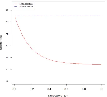
Figure 3.1 shows the result of a defaultable call and put option in comparison to the
Black-Figure 3.1: Defaultable call and put option prices against Black-Scholes option prices with
r= 2%,S = K = $35,R= 70%,σ=18%,T =5, with a 99% confidence level.
Scholes results of the two non defaultable options. An increase in the default rate causes the
option price to drop dramatically. What we can also notice is when the default rate is closer to
zero, the defaultable options almost reach the Black-Scholes risk neutral prices. This will be
further investigated in Chapter 4. Now in Figure 3.2 with the same results and simulation steps,
Figure 3.2: Defaultable call and put option prices with r = 0%, S = K = $35, σ = 18%,
R=70%,T = 5, for error bars of the simulations refer to Appendix C, Figure C.1.
and call option prices are essentially the same except some minor differences due to simulation error. It can be seen that the Put-Call parity holds well here even for defaultable option.
3.4
Analytical Approximation for Defaultable Option Prices
To see how accurate our simulations are we have decided to further proceed in finding an
analytical solution to our simulations. There are always errors in using Monte Carlo methods so
if we can find an analytical solution of our defaultable option we can then compare the results.
In this chapter we propose an analytical approximation to pricing defaultable options which
we have not seen in the literature. A closed form solution consists of solving the following
formula:
e−rTE[f(ST)Iτ≤T]+e
−rT
3.4. AnalyticalApproximation forDefaultableOptionPrices 29
In the equation (3.13), f(ST) is simply an option function evaluated atT, time to maturity and
the indicator functionIrepresents a 1 if default happens withinT or a 0 otherwise.ris the risk
free interest rate with which we discount values to find the option price att = 0. The formula can then be expanded to the option function of a call. Whenτ≤T then:
f(ST)= R[(Sτ−K)+e r(T−τ)].
(3.14)
Whenτ >T then:
f(ST)= (ST −K)+. (3.15)
Now we can bring together the two cases shown in equation (3.14) and (3.15) above, and plug
them into equation (3.13). The results will give us the following:
e−r(T)E[R(Sτ−K)+er(T−τ)Iτ≤T]+e−rTE[(ST −K)+Iτ>T]
=E[R(Sτ−K)+e−rτIτ≤T]+e−rTE[(ST −K)+Iτ>T]
=RE[E[R(Sτ−K)+e−rτ|τ=t1,t1≤ T]]+e−rTE[E[(ST −K)+|τ=t1,t1 >T]]. (3.16)
LetCBS(T) andCBS(τ) represent the call option function calculated at T and τ, respectively.
So now once we substitute in (3.16) the actual option function of Black Scholes we get:
RE[CBS(τ)|τ=t1,t1≤ T]]+e−rTE[(ST −K)+]E[I|τ= t1,t1 >T]. (3.17)
Because of independence in the second part of the equation, we were able to separate the
expectation into two parts allowing us to use the basic Black-Scholes formula at time T for
part of the evaluation. This will be denoted byCBS(T), which is the Black-Scholes formula for
a call option in a risk neutral world. Now we need to replace the indicator functions with actual
default probabilities and as stated above the waiting time until the first arrival of a default is
represented by an exponential distribution which will change formula (3.17) in the following
way:
R
Z T
0
CBS(τ)Pλ(τ)dτ+CBS(T)
Z ∞
τ=T
where:
Pλ(τ)=λe−λτ.
To solve equation (3.18), we first looked at a simple case of using a Taylor series
approxima-tion to expand the standard normal distribuapproxima-tion that is in the Black-Scholes formula. During
these works we realized that there are a few different ways to get such solutions depending on how versatile we would like our analytical results to be. These results will be explained and
compared in the following sections.
3.4.1
Taylor Series Approximation Method for Standard Normal
First for simplicity we will number two parts of equation (3.18), so we can simply identify
them:
R
Z T
0
CBS(τ)Pλ(τ)dτ, (3.19)
CBS(T)
Z ∞
τ=T
Pλ(τ)dτ (3.20)
Before we proceed further into solving with Taylor Series approximation notice that equation
(3.20) is a simple integral which we can solve in closed form. Equation (3.20) will give us the
following:
CBS(T)
Z ∞
τ=T
Pλ(τ)dτ
=CBS(T)
Z ∞
τ=T
λe−λτdτ
=CBS(T)e−λT. (3.21)
In equation (3.21) notice how our result is simply a Black-Scholes formula multiplied by the
probability that the default did not happen in the intervals 0 and T. Now we move to the more
complex case which is shown in equation (3.19):
R
Z T
0
CBS(τ)Pλ(τ)dτ
= R
Z T
0
CBS(τ)λe
3.4. AnalyticalApproximation forDefaultableOptionPrices 31
= R
Z T
0
[S N(d1(τ))−N(d2(τ))Ke−rτ]λe−λτdτ. (3.22)
If we letr = 0% and S0 = K it will help us in the approximation since in this setting (2.23) and (2.24) reduce to:
d1(τ)= 1 2σ
√
T, (3.23)
d2(τ)=−d1(τ). (3.24)
We then use a Taylor Series Expansion for the standard normal distributions that we have in
our Black Scholes formulaN(.):
N(x)= N(0)+N0(0)x+N00(0)x 2
2 +O(x 3).
(3.25)
We apply results of (3.23) and (3.24) to our Taylor Series in (3.25). The call option atτcan now
be represented through a Taylor Series approximation in this way (Notice: many cancellations
have happened here due to makingS = Ke−r(T−t)):
CBS(τ)= S[N(d1(τ))−N(−d1(τ))]
=S[N(0)+N0(0)d1(τ)+N
00
(0)d2(τ) 2
2 −N(0)+N
0
(0)(−d1(τ))+N
00
(0)d2(τ) 2
2 ]
= S[2N0(0)d1(τ)]
= S[N0(0)σ√τ],
where
N0(0)= √1
2π.
LetQ= N0(0) for simplicity, since it will be carried through our calculations. Now:
CBS(τ)= S Qσ √
We can now calculate the integral represented in equation (3.19) by inputting the equation
(3.26) which results in:
R
Z T
0
CBS(τ)Pλ(τ)dτ= RσλS Q
Z T
0
√
τe−λτdτ.
By changing variables, letting some variablex= √τit results in the following integral:
RσλS Q
Z
√
T
0
2x2λe−λx2dx.
Then, we apply integration by parts where we let:
v= x,
du= −2xλe−λx2dx.
Solving the integration by parts gives us the following results:
−RσS Q[
√
T e−λT −
Z
√
T
0
e−λx2dx]. (3.27)
Since we are looking at a closed form solution, notice how the integral R
√
T
0 e
−λx2dx is quite
similar to the error function. The error function is:
erf(x)= √2
π Z x
0
e−t2dt.
Error function can also be represented through the cumulative distribution, given byN(.), which
is the integral of the standard normal distribution, the relationship is: