Mobile Robot Homing Control Based on Odor Sensing.

(1)

Abstract

CRAVER, MATTHEW DAVID. Mobile Robot Homing Control Based on Odor Sensing. (Under the direction of Edward Grant.)

As robotic systems transition fully out of the laboratory environment and into the real world, they will need to be more robust and autonomous in order to deal with different environmental conditions and increasing complex tasks. Many developers have attempted to solve this problem by using increasingly more sensors and computational resources to provide the control system with more information. Others have tried to more explicitly define the environment and task being performed. However, there are many relatively simple biological organisms that exhibit complex behaviors using limited resources. This dissertation reports on the use of a biologically-based solution to develop a robotic platform and control system that allow for emergent intelligence and robustness.

A new robotic platform, the EvBot III, was developed with ubiquitous modularity in software, hard-ware, and control systems as a goal. The EvBot III is comprised of (1) a differential drive base with an attached turret and sensor shield, (2) a StackableUSB™ single board PC-104 computer, (3) a gen-eral purpose data acquisition system (CRIM-Daq), (4) a modular control architecture [1], and (5) a 3D physics-enabled simulation environment [2]. The driving portion of the base is designed such that dif-ferent drive systems (legged system, ackerman drive, etc.) can be used without needing to change the main controller. Additionally, the sensor shield allows different configurations and sensing modalities to be switched out based upon the desired application. Therefore, the EvBot III is expected to decrease development time and accelerate the progress of robotic and computational intelligence research.

(2)

(3)

Mobile Robot Homing Control Based on Odor Sensing

by

Matthew David Craver

A dissertation submitted to the Graduate Faculty of North Carolina State University

in partial fulfillment of the requirements for the Degree of

Doctor of Philosophy

Computer Engineering

Raleigh, North Carolina

2014

APPROVED BY:

Troy Nagle Coby Schal

Wesley Snyder Edward Grant

(4)

Dedication

(5)

Biography

(6)

Acknowledgements

I would first like to thank my family for always being there to support me. They have always encouraged my curiosity and questioning, and have given me the strength to excel in everything I do.

I would need to express my sincere gratitude to my advisor Dr. Edward Grant for bringing me into the Center for Robotics and Intelligent Machines (CRIM) and continually supporting me and show-ing confidence in my ability. Additionally, I would like to acknowledge the other members of my committee– Dr. Colby Schal, Dr. Wesley Snyder, and Dr. Troy Nagle–for their assistance.

I also need to thank the many members of the CRIM who have mentored and helped me throughout my graduate career. Dr. Kyle Luthy, Brooks Adcock, Frederick Livingston, Dr. Leonardo Mattos, Dr. Nikhil Deshpande, Micah Colon, Jim Ashcraft, Zack Nienstedt, Mark Draelos, and Chris Bollinger have served as a sounding board and provided valuable input to this work.

Additionally I would like to thank Zane Purvis and Ben Stiles for providing assistance with code and design issues.

(7)

Table of Contents

List of Tables . . . x

List of Figures . . . xi

Chapter 1 Motivation for Research . . . 1

Chapter 2 An Overview of Sensor Fusion Methods and Architectures . . . 3

2.1 Abstract . . . 3

2.2 Introduction . . . 3

2.3 Methods of Sensor Fusion . . . 5

2.4 Information Management . . . 7

2.5 Models of Sensor Fusion . . . 7

2.6 Techniques for Data Management . . . 9

2.7 Discussion . . . 11

2.8 Conclusion . . . 13

Chapter 3 A General-Purpose Mobile Robotic Platform: EvBot III Hardware and Soft-ware Architecture Design . . . 14

3.1 Abstract . . . 14

3.3 The EvBot Platform . . . 15

3.3.1 EvBot I and EvBot II . . . 16

3.3.2 EvBot III . . . 17

3.4 Base and Charging Station Design . . . 17

3.4.1 EvBot III Base . . . 17

3.4.2 OceanServer Power Solution . . . 19

3.4.3 Portable Charging Station . . . 19

3.5 Hardware Design (CRIM-Daq) . . . 20

3.5.1 CRIM-Daq Daughter Boards . . . 21

3.6 Software Design . . . 24

3.6.1 Linux Build Tree . . . 24

3.6.2 EvBot III Firmware . . . 24

3.6.3 Simulation Environment . . . 25

3.8 Conclusion . . . 26

Chapter 4 Chemical Sensing for Mobile Robots: An Improved Method for Implementa-tion in Dynamic Indoor Environments . . . 27

4.1 Abstract . . . 27

4.2.1 Passively-Sampled Chemical Sensors . . . 28

4.2.2 Wind Direction Sensor with Passively-Sampled Chemical Sensors . . . 31

(8)

4.2.4 Problems with Robotic Chemical Sensors . . . 37

4.3 Desecription of EvBot III Testbed . . . 37

4.3.1 Robotic Platform . . . 37

4.3.2 Testing Arena . . . 38

4.4 Experiment 1 . . . 39

4.4.1 Methods . . . 39

4.4.2 Results . . . 41

4.5.1 Methods . . . 41

4.5.2 Results . . . 41

4.6.1 Methods . . . 42

4.6.2 Results . . . 43

Chapter 5 Odor Sensorimotor Control Software Implementation, Testing, and Analysis . . . 46

5.1 Abstract . . . 46

5.3 Design . . . 47

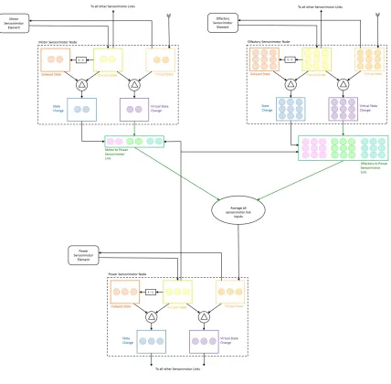
5.3.1 Overview of the EvBot III Sensorimotor Network . . . 49

5.3.2 Implementation of the EvBot III Sensorimotor Network . . . 50

5.4 Training and Testing the EvBot III Sensorimotor Network . . . 56

5.4.1 Random Movement Generation . . . 56

5.5.1 Methods . . . 58

5.5.2 Results . . . 58

5.6.1 Methods . . . 58

5.6.2 Results . . . 58

5.7 Experiments 3 and 4 . . . 59

5.7.1 Methods . . . 59

5.7.2 Results . . . 59

5.8 Experiment 5 and 6 . . . 60

5.8.1 Methods . . . 60

5.8.2 Results . . . 61

5.9.1 Methods . . . 61

5.9.2 Results . . . 62

5.10 Experiment 8 . . . 63

5.10.1 Methods . . . 63

5.10.2 Results . . . 63

5.11 WEKA . . . 64

(9)

Chapter 6 Summary of Findings . . . 90

References . . . 94

Appendices . . . 107

Appendix A Sensorimotor Network Mathematical description . . . 108

Appendix B All LabVIEW Sensorimotor Inputs . . . 110

Appendix C CRIM-Daq . . . 113

C.1 CRIM-Daq Schematic . . . 114

Appendix D CRIM-Daq Motor Control Board . . . 120

D.1 CRIM-Daq Motor Control Board Schematic . . . 121

D.2 CRIM-Daq Motor Control Board Layout . . . 125

Appendix E CRIM-Daq Inertial Measurement Unit . . . 126

E.1 CRIM-Daq Inertial Measurement Unit Schematic . . . 127

E.2 CRIM-Daq Inertial Measurement Unit Board Layout . . . 130

Appendix F CRIM-Daq Serial Analog to Digital Converter Board . . . 131

F.1 CRIM-Daq Serial Analog to Digital Converter Board Schematic . . . 132

(10)

List of Tables

Table 2.1 DARPA Grand Challenge Winners . . . 4

Table 3.1 Inexpensive Robotic Platforms . . . 15

Table 3.2 Common Research Robotic Platforms . . . 15

Table 4.1 Summary of Approaches to Robotic Airborne Chemical Sensing . . . 29

Table 4.2 Sensor Configuration 1 with Vector Summing Homing Algorithm . . . 41

Table 4.3 Sensor Configuration 2 with Vector Summing Homing Algorithm . . . 42

Table 4.4 Sensor Configuration 2 with Sensor Normalization and Vector Summing Homing Algorithm . . . 43

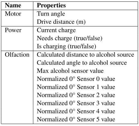
Table 5.1 Sensorimotor Modalities and Their Components . . . 49

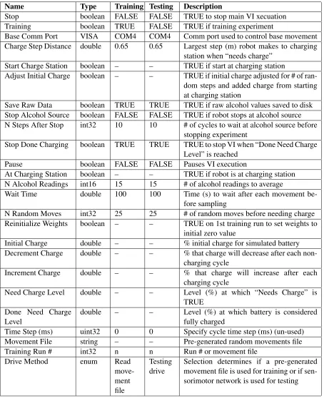
Table 5.2 EvBot Sensorimotor Network LabVIEW Commonly Used Inputs . . . 54

Table 5.3 EvBot Sensorimotor Network LabVIEW Outputs . . . 55

Table 5.4 Sensorimotor Link Weight Sizes . . . 56

(11)

List of Figures

Figure 2.1 McIntyre’s Comprehensive Sensor Management and Scheduling Model . . . 10

Figure 2.2 Schaefer’s Sensor Rich Environment Sensor Management System . . . 11

Figure 2.3 General Controller Architecture [3] . . . 11

Figure 2.4 Sensorimotor Neuronal Interface [3] . . . 12

Figure 3.1 EvBot Platform . . . 16

Figure 3.2 EvBot III base design model . . . 18

Figure 3.3 EvBot III Portable Charging Components . . . 20

Figure 3.4 CRIM-Daq with labeled components . . . 21

Figure 3.5 CRIM-Daq Daughter Boards . . . 23

Figure 3.6 RoboClaw 2x30A Motor Controller . . . 23

Figure 4.1 Reactive Autonomous Testbed (RAT) . . . 31

Figure 4.2 Orebro Mark II Mobile Nose . . . .¨ 31

Figure 4.3 Robot Testbed used by Ishida et al. . . 34

Figure 4.4 Testbed used by by Ishida et al. . . 34

Figure 4.5 Mark III Mobile Nose on a Koala Robot . . . 36

Figure 4.6 Mark III Mobile Nose Schematic . . . 36

Figure 4.7 EvBot III Olfactory Sensor Shields . . . 38

Figure 4.8 Arena with Alcohol Plume . . . 39

Figure 4.9 Simulation of Alcohol Plume . . . 40

Figure 4.10 Alcohol Plume Source . . . 40

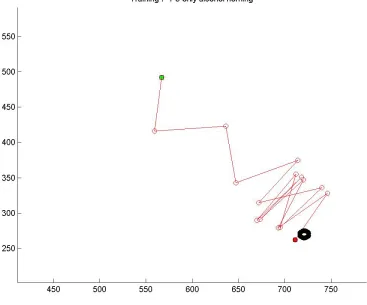
Figure 4.11 Training 7-1-5 EvBot Alcohol Homing Movement . . . 44

Figure 5.1 Sensorimotor Network . . . 48

Figure 5.2 EvBot Sensorimotor Network LabVIEW Block Diagram . . . 51

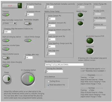
Figure 5.3 Complete EvBot Sensorimotor Network LabVIEW Front Panel . . . 52

Figure 5.4 Commonly Used Portion of LabVIEW Sensorimotor Network Front Panel . . . . 53

Figure 5.5 Sensorimotor Network Flow Chart . . . 55

Figure 5.6 Training/Testing Arena . . . 57

Figure 5.7 Testing 1-7 EvBot movement . . . 65

Figure 5.8 Training 1-7 Sensorimotor Weights . . . 66

Figure 5.9 Testing 2-1 EvBot movement . . . 67

Figure 5.10 Training 2-2-19 Sensorimotor Weights . . . 68

Figure 5.11 Testing 4-3-19, run 0, EvBot movement . . . 69

Figure 5.17 Testing 6-1-9, run 0 no alcohol, EvBot movement . . . 75

(12)

(13)

Chapter 1

Motivation for Research

Mobile robots have shown great promise for aiding humans in dangerous situations such as search and rescue at disaster sites [4–7], industrial applications [8, 9], security monitoring [10, 11], and for performing tasks remotely in a natural environment [12, 13]. While these applications are dynamic in nature, many robotic systems require a constrained environment [14]. Due to the lack of hard constraints in real-world applications, it can be difficult to plan and program such systems for all eventualities.

In order to provide robots with more information so that appropriate control decisions can be made, many groups have increased the number of sensors on their mobile platforms [15–17]. For example, the winner of the DARPA Grand Challenge used 5 SICK laser range finders, 1 color camera, 2 24GHz RADAR sensors, a GPS positioning system, a GPS compass, and a 6-axis IMU to navigate an off-road course [15]. While the technology that has come out of the DARPA Grand Challenge has shown significant leaps in autonomous vehicle navigation [15–17], its extreme cost and complexity limits its use [18, 19]. Additionally, it is impractical to use large numbers of sensors on mobile robots due to the significant processing demands. For example, the vehicle that won the DARPA Grand Challenge required 6 Pentium M computers (2 executed the race software, 1 performed vision processing, 1 logged the race data, and 2 were idle) [15]. The power demands of these sensors also render them infeasible for use on small mobile platforms relying on limited battery power.

Other groups have attempted to constrain the robotic system by explicitly choosing the base behav-iors that the robot will need to perform a task in a given environment [3, 20–23]. This can lead to a system that is overly constrained by experimenter bias [3]. Problems can arise if all eventualities are not taken into account. For example, obstacle avoidance is often presumed to be a base behavior in robotics. Conversely, it has been shown that obstacle avoidance can be considered to be an emergent or derivative behavior of homing [24, 25].

(14)

platform [26, 27], which suffered from limited battery life, drive train slippage, etc. The new EvBot III also has enhanced modularity and scalability. In order to reduce sensor complexity, only chemical sen-sors were used. Olfaction was selected over other modalities (vision, touch, etc.) because the response to chemical stimuli was the first sense developed by primordial life [28]. Additionally, although olfaction is the most widespread sensory modality found in nature, it is the least often implemented in robotic sys-tems despite its potential for widespread application in the field of robotics [28]. Robotic olfaction can be used to find chemical leaks, explosives, or disaster victims [28]. In order to reduce experimenter bias and “provide stable even if non-optimal solutions in the face of uncertainty, noise or incomplete input, or unpredictable changes in context [3]”, the main robotic controller was implemented using a senso-rimotor integration architecture. This sensosenso-rimotor architecture is a flat, homogeneous architecture that fully connects all sensor and motor elements without internal distinction between the two. Throughout the training of the sensorimotor network, correlations in activities are built between all nodes. After training, these correlations are used to drive the robot. In order to test the EvBot III’s performance, the robot was evaluated based upon its ability to autonomously navigate up an alcohol plume to a charging station.

(15)

Chapter 2

An Overview of Sensor Fusion

Methods and Architectures

2.1 Abstract

Robotic systems are currently being used to perform increasingly complex tasks. This has resulted in an abundance of data that is available to the control system, and consequently a growing need for methods to pick out and combine the most appropriate data. Sensor fusion methods are a common method used for fusing the output of sensors with different modalities. This reduces the amount of data that the control system needs to process. There are also sensor fusion architectures that incorporate mission management functions to help the system intelligently use the fused data. Additionally, biologically-inspired sensorimotor networks offer the ability to autonomously fuse the various sensor data and apply the fused data to generate emergent behavior. Given the complexity and variety of sensors in the natural realm, these biologically inspired sensorimotor networks are poised to truly launch autonomous systems out of the laboratory and into the real world. This chapter provides an overview of the various methods used for reducing the amount and complexity data.

2.2 Introduction

(16)

Table 2.1: DARPA Grand Challenge Winners [15–17]

Team Sensors Computation

1st Place

Stanford Racing Team, Stanley

(Stanford University)

5 SICK laser range finders, 1 color camera, 2 24GHz RADAR sensors, GPS positioning system, GPS Compass, 6-axis IMU

6 Pentium M comput-ers (2 executed race software, 1 performed vision processing, 1 logged race data, and 2 were idle

2nd Place

Red Team, Sandstorm (Carnegie Mellon Univ.)

1 Riegal Q140i scanning laser range finder, 3 SICK LMS laser scanners, 1 high speed stereo vision system, 1 NavTech DS2000 Continuous Wave Frequency Modulated radar, 1 Applaniz POS-LV pose estima-tion system (Inertia measurement, GPS, odometry)

1 quad processor Ita-nium II, 3 dual proces-sor Xeon, 4 Pentium III class PC-104s

3rd Place

Red Team, H1ghlander (Carnegie Mellon Univ.)

1 Riegal Q140i scanning laser range finder, 6 laser scanners, 1 Applaniz POS-LV pose es-timation system (Inertia measurement, GPS, odometry), 1 high speed stereo vision system

7 Pentium M computers

that data so that intelligent control decisions can be made. As a result of this “information overload”, it is becoming more difficult for the designers to explicitly describe the correlations between the many different sensory and mechanical components of the system [30].

Conversely, biological systems are capable of efficiently using data from a variety of sensing modali-ties (vision, auditory, tactile, etc.) to make intelligent control decisions [31]. The sensorimotor system of these organisms is integral in the coordination of sensory and motor activities, giving rise to bodily sta-bility [32]. These systems remain flexible and adaptive to different environments and situations through complementary relationships between the static and dynamic components at the system level [33].

(17)

architectures are needed, and these are presented (Section 2.4). Finally, guidance for managing the sys-tem models and applying sensor fusion techniques to the control of mobile robots is provided (Section 2.6). Particular attention is paid to sensorimotor integration.

2.3 Methods of Sensor Fusion

The most comprehensive definition of data fusion is given by Abidi and Gonzales as “the synergistic combination of information made available by various knowledge sources such as sensors, in order to provide a better understanding of a given scene” [34]. Methods of sensor fusion range from using the sensor with the modality best suited for each particular type of measurement (i.e., using pulsed radar to determine an aircraft’s range, and using forward-looking infrared imaging to determine its angular direction [31]) to using fuzzy techniques to combine the sensor outputs, or to creating “virtual sensors” by combining and processing the output of multiple sensors.

Multi-Sensor Data Fusion (MSDF) encompasses the detection, association, correlation, estimation, and combination of data from a multitude of sensors. MSDF can be used to overcome sensor uncertainty, increase reliability, and provide better resolution. This technique involves data preprocessing, sensor modeling and estimation, data association, and data fusion [35, 36]. The result of this process is an optimal estimate of a particular state vector that relates to a specific component of the observed system (i.e., a state vector for the vision system, for the tactile system, etc.) [35]. Because MSDF systems also account for both spatial and temporal resolution with regard to the rated resolution of each element, they can be used to create a system that can gracefully deal with the gradual degradation or failure of its components [35].

In order to accurately model a system, a dynamic working description of its constituent sensors must first be constructed [35]. This process involves converting all of the raw sensor data into a “com-mon language” [37]. This is accomplished by modeling the sensor’s error characteristics that classify and describe a given measurement [38]. Then, an estimator or tracker must be found that can provide an acceptable estimate of sensor uncertainty. Conventionally, a Bayesian approach is used [39–41]. This is often implemented using an extended Kalman filter, although a more effective method utilizes informa-tion metric-based estimators [35].

(18)

Information metrics can also be used to evaluate and compare the available information in any multi-sensor system [42].TheFisher information metricis a particular type of information metric that can be used to characterize the statistical difference between observations. This measurement is found by calculating the moments of the observed data. For non-random parameters, the Fisher information matrix is defined in terms of likelihood; it holds true for both single and random variables [42].

In systems with multiple sensors and sensing modalities, the performance of the system can often be improved by combining the incoming data in a meaningful and productive manner. Towards this end, many different sensor fusion techniques have been proposed that combine, relate, and correlate the raw sensor data. Following are descriptions of the more widely used sensor fusion techniques.

Isolation fusersare among the most important fusing methods. They introduced theisolation prop-erty, which is used as a metric to compare and contrast nearly all other fusing methodologies [45–47]. The isolation property ensures that the information gained by fusing the data from the individual sen-sors is at least as complete and correct as the information available from each of the best individual sensors [45–47]. If this property is not fulfilled, then fusing the data is of limited to no benefit.

The linear fuser is one of the most basic sensor fusion methods. Here, the sensor’s outputs are simply summed; this action satisfies the isolation property. Theoptimal linear fuserimproves upon the linear fuser by minimizing the expected error. However, the optimal linear combination fuser requires that the sensors be equally distributed around certain global values; this is often difficult to realize in actual systems [44,45]. Theprojective fuseris another expansion of the linear fuser. The projective fuser computes the error regressions of the sensors and transfers the output of the sensor to correspond to the lower envelope of regressions for every point [45, 48].

(19)

2.4 Information Management

In order to efficiently apply the fused sensor information for learning new behaviors and accomplishing specific tasks, a global management architecture is needed. This architecture also allows the behaviors and actions of the system to be correlated with the environment (as represented by the sensory system). Information request prioritizationis one of the most common methods of information-oriented man-agement. Implementation of this method requires that certain sensors be given a higher priority when making control decisions for a unique set of conditions. This priority is determined from current mission and situational awareness, as gleaned from previous sensor readings and evaluations [49–52]. The sens-ing actions selectionmethod extends upon the information request prioritization method by prioritizing the resources that are allocated to each sensing action. By limiting sensor resource allocation in addition to data selection, informational gain is maximized and resource allocation is minimized with respect to all levels of information acquisition [53–56].

The descriptively named method ofadding sensing resources for added quality of fused information deploys additional sensing resources with the hope that the quality of the fused information will be enhanced [53]. Systems using this method typically operate in dynamic environments because more sensors are needed to adequately represent changes in the surrounding conditions [57–59]. However, more resources are needed to allow for the use of this increased set of sensing capabilities.

The focus of attention strategy also provides a good option in terms of resource utilization and performance. This strategy attempts to reduce the quantity of the data processed by the sensory system while increasing its informational value. This is accomplished by providing the system with the correctly associated sensor measurements (versus providing the system with all available information, correlating it all, and later using the measurements that are correctly correlated) [42]. One specific instance of the focus of attention strategy isview selection. Although view selection is best suited for vision search applications, it can also be applied to other “concrete” sensing modalities (i.e., acoustic and tactile modalities). The view selection technique chooses viewing locations and directions in order to improve the utility of the information gained from the sensing resources [53, 60]. It also decreases the number of resources that are required from the operating system by utilizing a narrower, more specifically focused view of the environment.

2.5 Models of Sensor Fusion

(20)

The probability distributions of the sensors themselves can be used to relate the sensor’s output to a desired feature in the external environment [45]. For example, the data of fused sensors is often grouped based upon the modalities that they can most accurately measure individually. Therefore, knowledge of the probability distributions allow the system to generate an effective internal representation of the external environment [45].

Another technique for reducing dataset complexity isPrinciple Component Analysis(PCA). PCA involves transforming the set of possible correlated variables into a smaller set of uncorrelated variables (i.e., principle components). Once these principle components are isolated, any redundant data is no longer considered for the computation of control. This allows the dataset to be greatly simplified and reduces the resources necessary for computation and control [61].

The Adaptive Spline Modeling (ASMOD) algorithm is an example of a model that includes the provision for adaptation. In order to allow for adaptive behavior, the ASMOD algorithm creates a set of different models, each of which correspond to a certain specific set of “candidate refinements” [35]. These candidate refinements can be categorized as either model building or model pruning. Then, the candidate model that produces the largest improvement in when approximating the external environment is selected [35].

There are three categories of model building refinements that are associated with the ASMOD al-gorithm: univariate addition, sensor multiplication, and knot insertion.Univariate additionsimply in-corporates a new, one-dimensional submodel with a new input variable into the existing ASMOD al-gorithm [35]. The incorporation of this submodel allows the updated alal-gorithm to additively model the new variable and its correlations to the external environment [35]. Sensor multiplicationreplaces the current ASMOD algorithm with a new algorithm whose result is dependent upon the addition of at least one new input variable; this contrasts with univariate addition, which simply inserts a new input variable into the current algorithm. As a result, the sensor multiplication model can describe the coupled depen-dencies between combined input variables [35]. Theknot insertionmodel is the most computationally intensive of the building refinements. It inserts a new basis function(s), or equivalent rule(s), in order to increase the flexibility of the ASMOD submodel [35].

(21)

2.6 Techniques for Data Management

Similar methods of data management are also used with sensor fusion models. However, these tech-niques represent higher-level management that must combine the information available from a number of sensors (both real and virtual) or modalities. Many of these models use dynamic coupling, which finds its roots in the field of Embodied AI. Dynamic coupling allows the “external” environment to be expanded to include, not only those features outside of the control system’s physical realization, but also the system’s internal representation of itself and associated states [62].

In addition to the typical physical sensors and detectors that make up sensory systems,virtual sen-sorscan be constructed to expand the sensing capabilities of a system. Virtual sensors add a layer of software abstraction that allows for computationally-constructed data to be treated as if it came from a real device. This provides for a simple and consistent view of the various input devices. Software and data filters are common examples of virtual sensors. With respect to sensor fusion, the data from two or more detectors can be combined to createphantom device data. Phantom device data consists of data from a real device’s inputs that are shaped by a set of constraints [43, 63].

Thecross modal mapcombines many of the aforementioned models and methods of sensor fusion. The cross modal map describes the correlative mapping between different modalities of input (i.e., physical sensors, virtual sensors, and otherwise) and highlights issues related to evaluating the data from different sensory sources. These evaluations are necessary if any worthwhile correlations between the different data are to be found.

McIntyre and Hintz developed another model for sensor fusion systems that expands on the idea of information-oriented management (Figure 2.1) [64]. In their model, a mission manager mediates requests made by a human operator. At the most basic level, the mission manager functions as a feed-back control system that continually monitors the state of the sensors in order to ensure optimal perfor-mance [65]. The mission manager also maintains the mission goals and objectives, which are determined a priori and offline, although they can be modified in real-time and stored. Put simply, the mission man-ager only cares that goals are accomplished and measurements are made relative to a set of priority and temporal constraints; the mission manager does not care which specific sensor(s) or measurement meth-ods are used [30,52,64,65]. In this model’s hierarchy, the fusion space is simply where the sensor fusion takes place using the prescribed technique(s). The information space contains the sensor manager and mission manager. It also converts the sensor data, which is related to the current state of the observed environment, into to its internal, mathematical representation [30].

(22)

ad-Figure 2.1: GMU Sensor Management and Scheduling Model [64]

dition of sensors without provisions for processing this information (i.e., “data overload”) [30]. Here, the mission and sensor managers operate independently, with the sensor manager serving to convert the mission goals to information needs on an as-needed basis [30]. Furthermore, depending upon the scien-tific nature of the environment or situation, simply implementing a sensor manager without a mission manager may be sufficient [64].

(23)

Figure 2.2: Sensor Rich Environment Sensor Management System [30]

Figure 2.3: General Controller Architecture [3]

2.7 Discussion

(24)

Figure 2.4: Sensorimotor Neuronal Interface [3]

(25)

This chapter has also reviewed some of the available architectures for sensor fusion mission manage-ment such as the information-oriented managemanage-ment developed by McIntyre and Hintz [64], the Sensor Rich Environment Sensor Management System proposed by Schaefer and Hintz [30], and the Sensori-motor Integration architecture developed by Bovet and Pfeifer [3, 66]. The main advantage of mission management architectures is that they operate as a feedback control mechanism between the mission goals and objectives, and the actual sensors and systems. They provide an up-to-date internal mathe-matical representation of the system and its performance. However, this also highlights one potential disadvantage, namely that they must have an accurate model of the internal and external environments. This is often difficult, if not impossible, to obtain in all but the simplest environments.

2.8 Conclusion

Many of the systems and methods described in the review require extensive knowledge of the physical sensors and environments in which they are operating. Often, this is not feasible in dynamic environ-ments that require continual updating of internal models. Additionally, sensor loss or degradation can become an issue. In order to limit the chance of incorrect characterizations that can overly constrain the system and provide additional sources of error, architectures such as the sensorimotor system described by Bovet and Pfeifer [3, 66] should be used.

(26)

Chapter 3

A General-Purpose Mobile Robotic

Platform: EvBot III Hardware and

Software Architecture Design

3.1 Abstract

This chapter describes the design of the EvBot (Evolutionary Robot) III general purpose robotic re-search platform. The EvBot III was designed around the idea of ubiquitous modularity in software, hardware, and control systems. The EvBot III research platform is comprised of (1) a differential drive base with an attached turret and sensor shield, (2) a StackableUSB™ single board PC-104 computer, (3) a general purpose data acquisition system (CRIM-Daq), (4) a modular control architecture [1], and (5) a modular 3-D physics-enabled simulation environment [2]. The EvBot III has the potential to decrease development time and accelerate the progress of robotic and computational intelligence research.

3.2 Introduction

Mobile robot bases can be broadly characterized as (1) small and inexpensive with limited computa-tional resources or (2) large and expensive with advanced computacomputa-tional resources. The most common inexpensive mobile robots are listed in Table 3.1. Because some of these platforms (i.e., EV3, VEX, VEX IQ, and TETRIX) are packaged as general purpose kits that can be used to construct a variety of robots, they have the advantage of being easily reconfigurable. The main disadvantage of these systems is their limited computational resources. Of the smaller, more inexpensive platforms, the Turtlebot 2 holds the most promise as a research tool because it comes with a netbook and a Microsoft Kinect.

(27)

dis-Table 3.1: Inexpensive Robotic Platforms [68, 69]

Lego Mindstorms EV3 $350

Mobsya Thymio II $190

iRobot Create $130

Turtlebot 2 $1995

(Built on the iRobot Create)

Vex Robotics VEX IQ $250

Vex Robotics VEX $400

TETRIX $380

Surveyor SRV-1 $495

Table 3.2: Common Research Robotic Platforms [68, 69]

Khepera $3200

Koala $8400

Pioneer P3-DX $4000

cussed. The prices provided in Table 3.2 reflect those for the base and the basic computing power needed to drive the robot [68, 69]. The overall cost of these platforms quickly rises with the addition of an on-board computer and peripheral sensors. For example, Jeanne Dietsch of MobileRobots noted that the actual cost of the Pioneer P3-DX is around $19000when the advanced laser mapping and autonomous navigation software, laser bumpers, gyros, and wireless communication hardware are added [70].

3.3 The EvBot Platform

(28)

(a) EvBot I (b) EvBot II (c) EvBot III

Figure 3.1: EvBot Platform

3.3.1 EvBot I and EvBot II

The EvBot I [26] and EvBot II [27] have been used to complete a number of different projects that have displayed the platform’s versatility. These projects have included: (1) evaluating evolved neural controllers [14,71–77], (2) using an acoustic array to test UAV control algorithms for passively detecting and locating a variety of radar sources [78,79], (3) using an omnidirectional vision system for formation control [80], (4) serving as a test bed for optical robotic communications [81], (5) testing algorithms for smart sensor networks [82–84], and (6) repairing randomly distributed sensor networks [85].

(29)

Although immensely important for training and testing, the Matlab simulation environment is also limited. The simulation environment was not created with modularity as its primary goal. For example, it was limited to the 2-D maze environment, which confined the EvBot to lab use only. The addition of new sensor modalities (i.e., the acoustic array) was also unfeasible. The simulation environment was further limited by the lack of a governing physics model.

3.3.2 EvBot III

In order to address the issues outlined above, the EvBot III has been designed to be more modular both in terms of hardware and software. Other improvements include increased computational resources and more powerful batteries that have the ability to self-monitor and recharge autonomously.

In order to incorporate these features into the new EvBot III, a custom base was designed and built. Similar to the EvBot I and II, the EvBot III has continued to embrace the use of the USB standard for device data connections. This standard has shown good support for increased hardware modularity, and is used in the new general-purpose data acquisition system (CRIM-Daq) and embedded computer (StackableUSB™, Micro/sys, Inc.). The improvements to the EvBot III base are discussed more fully in Section 3.4, with rationale and recommendations provided in terms of design decisions, material selection, manufacturing, and assembly. Upgrades to the hardware, including a discussion of the CRIM-Daq and associated daughter boards, are detailed in Section 3.5.

In addition to these hardware improvements, the software has also been updated. These upgrades include a modular object-oriented control architecture, custom recompilable Linux build tree [1], and a new 3-D modular simulation environment [2]. The system’s increased software modularity provides more efficient lower-level interfaces and controller components. The new reconfigurable/recompilable custom Linux operating system excludes all unnecessary components from the rolled-out distribution, and supports real-time scheduling and processing components [1]. A brief discussion of the new Linux build tree and modular simulation environment is provided in Section 3.6.

3.4 Base and Charging Station Design

The motivating factors driving the redesign of the EvBot platform include the full embrace of both hard-ware and softhard-ware modularity, as well as precise measurement, control, and modeling of autonomous robotic systems. These factors, along with the overarching goal for use as a general-purpose research platform, have guided the design of the EvBot III base.

3.4.1 EvBot III Base

(30)

Figure 3.2: EvBot III base design model

Ultra-high-molecular-weight polyethylene (UHMW), laser-cut acrylic, 3D printed ABS thermoplastic, aluminum, and styrene. The UHMW was used for the majority of the base because it is easy to machine. The top and bottom were made using laser cut acrylic so that a person could easily see into the base. Aluminum was used for support elements and the center shaft of the slip-ring, and the 3D printed ABS thermoplastic was used in the brackets that attached the sensor shield to the base.

Drive train slippage was a major problem noted with the EvBot I and II bases [26, 27]. In order to address this in the redesign of the EvBot III, a differential drive system was used in combination with an actuated rotational platform. This new base allows for “holonomic” movement, where pseudo-holonomic is meant to indicate a system that appears pseudo-holonomic to an outside observer, although the underlying hardware is non-holonomic. A pseudo-holonomic design was chosen over a truly holonomic one in order to minimize design and development time, as well as keep future maintenance and upgrades as easy as possible. Pseudo-holonomic behavior is achieved using a turret in concert with an integrated slip-ring. The slip-ring allows for the transmission of DC power through the base using a standard 24-pin ATX power connector. Control signals from the base control system (located in the bottom portion of the base) are sent via USB or RS-232.

(31)

The EvBot III platform also allows new sensors to be added through the use of an outer shield that is attached to the actuated rotational platform (Fig. 3.2). The shield was made from styrene, which is both lightweight and inexpensive. External sensors can be mounted to the shield such that they remain in constant relative position regardless of the orientation of the rotating platform. Furthermore, the shield allows for easier implementation of the “focus of attention” method of sensor fusion [42]. The shield also makes the EvBot platform easier to simulate because it contains the entire base, including the drive wheels, and gives the EvBot a uniform circular outline.

3.4.2 OceanServer Power Solution

In order to address the power limitations present in the EvBot I and II, an OceanServer™ Intelligent Bat-tery and Power System (IBPS™) was used in the new EvBot III. The IBPS™ includes a MP-04SR/FR battery management module, a DC123SR DC-DC power supply module, and a BA-95HC Li-Ion smart battery pack. An EVAL233R USB-Serial module from FTDI was also added for monitoring and config-uring the battery system from the central computer.

The MP-04SR/FR battery management module can charge, discharge, and monitor up to four Li-Ion battery packs. It uses an RS-232 port to provide complete information about all connected battery packs. The information available for each connected battery includes, but is not limited to, current, voltage, amp-hours, run time to empty, and time to full charge. The MP-04SR/FR also seamlessly connects and delivers unregulated power to the DC123SR DC-DC converter module [86].

The DC123SR ultra high efficiency ATX DC-DC converter module supplies the following regulated DC voltages: +3.3V at 10A, +5V at 10A, +12V at 12A, and -12V at 12A. All of these conversions are done with greater than 95% efficiency [87]. Since each ring of the slip-ring in the EvBot III was only rated to 5A, it was not feasible to provide all of the regulated voltages to the top of the rotating platform. With 18 total rings available in the EvBot III slip-ring, 2 rings were used in parallel to provide +5V at 10A, and 3 rings were provided for each +12V at 12A and -12V at 12A to the top of the EvBot platform. The final IBPS™ component is the BA-95HC Li-Ion battery pack. Each battery pack has a 6.6Ah capacity with an unregulated output of 14.4V nominal [87]. The EvBot III base contains a removable compartment that can hold up to two of the BA-95HC batteries. If only one battery is installed, a place holder is used where the second battery would go.

3.4.3 Portable Charging Station

(32)

station, the shield of the charging station contains a hole with an LED that is at the same height as the camera hole of the EvBot, When the EvBot is aligned with the charging station, the LED is centered. The recharging process is monitored and controlled by the IBPS™ (Section 3.4.2).

(a) EvBot III Charging Station (b) EvBot III Charging Station’s Plug

(c) EvBot III (d) EvBot III Charging Receptacle

Figure 3.3: EvBot III Portable Charging Components

3.5 Hardware Design (CRIM-Daq)

(33)

low-level motor commands required to drive the base. In addition to robotics applications, the CRIM-Daq can be used for any project that requires data collection from one or more sensors; this is expected to reduce the production cost per board, and subsequently the cost of each new EvBot III.

The CRIM-Daq (Fig. 3.4) consists of a modified CRIM-Mote [88], an integrated ex430-f2013 pro-grammer/debugger (Texas Instruments), an integrated 4-port USB hub, and pass-through headers to allow for stackable expansion boards. The onboard CRIM-Mote circuit was modified to allow access to all of the I/O and signal pins from the msp430 using the pass-through headers. These headers give peripheral sensor boards access to 29 of the 32 possible general purpose I/O pins including two config-urable on-chip operational amplifiers, a 10-bit A/D converter, one UART, one IR communication port, one I2C port, and two SPI ports. A maximum of 112 individual nodes can be used on the I2C port, and a maximum of 22 nodes can be connected to the SPI port. Therefore, many different sensor boards can be connected to and used with the same Daq by stacking each on top of the pass-through head-ers. Then, once the msp430 is programmed with the application-specific code, all of the data from the attached sensor boards is accessible through the msp430 on the same USB port. The integrated ez430 programmer/debugger allows any code to be easily updated without any external hardware.

Figure 3.4: CRIM-Daq with labeled components

The CRIM-Daq can be either self-powered (i.e., an optional external power connection is included) or bus-powered. The board also includes circuitry to provide +3.3V, +5V, and±12V to any connected sensor boards. The circuitry to provide±12V was included to allow for use of differential input signals.

3.5.1 CRIM-Daq Daughter Boards

(34)

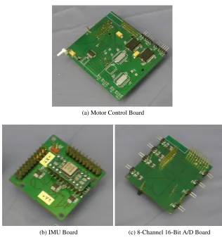
the circuitry required to interface with the shaft encoders of four motors, and the circuitry required to monitor the current sense output of each of the H-bridges.

The motors used to drive the EvBot III base (GHM-04, Lynxmotion) [89] have a2.5A stall current, and the H-bridges are rated to handle DC load currents up to5.0A [90]. However, after weeks of use, the CRIM-Daq motor driver board failed. The cause of these failures was later traced to the motors, which actually drew >20A when starting or changing directions. As a result the RoboClaw 2x30A motor controller (Fig. 3.6) was used to drive the base. The next revision of the CRIM-Daq motor driver will be updated to handle the increased current load.

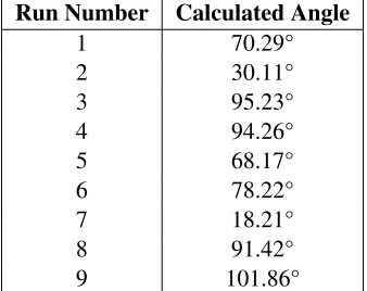
The Inertial Measurement Unit (IMU) was the second daughter board (Fig. 3.5b). This board is comprised of a 3-axis, ±3G accelerometer (ADXL330, Analog Devices) and a Z-axis gyroscope (ADXRS613, Analog Devices). In order to simplify the interface to the CRIM-Daq and ensure the tem-poral accuracy of the measurements, all of the sensor readings are transmitted to the CRIM-Daq through five serially-linked SPI ADCs with simultaneous sampling. Also, in order to increase the accuracy of the gyroscope, one of the ADCs is used to read in a temperature offset value so that the gyroscope can be calibrated.

The final daughter board is an 8-channel, 16-bit, 250 ksps A/D board (Fig. 3.5c). This board simul-taneously samples all 8 A/D channels and sequentially passes the data to the CRIM-Daq using SPI.

(35)

(a) Motor Control Board

(b) IMU Board (c) 8-Channel 16-Bit A/D Board

Figure 3.5: CRIM-Daq Daughter Boards

(36)

3.6 Software Design

3.6.1 Linux Build Tree

To begin the modularization of the software aspects of the control architecture, a new in-house Linux build tree [1] has been created that allows components to be added/removed before each new build. This enables greater flexibility when choosing new hardware components because the necessary drivers are included into the build tree, and the distribution rebuilt to suit the needs of any new mission scenario. This build system also allows for easier system upgrades when the Linux operating system kernel gets updated. Additionally, developers can continually incorporate new sensors, actuators, and other periph-eral devices as they are released and ported to Linux through kernel updates [1].

An object-oriented, modular control architecture [1] has also been developed. This architecture en-ables use by multiple developers and make the addition of new control structures more transparent (i.e., only small, hardware-specific adjustments will be needed). Also, because the architecture is object-oriented and modular, only minimal software modifications is needed to transfer it between different robotic platforms [1].

Currently, base objects are being created that will allow for the rapid development of controllers without the need to code modules to interface with the base hardware. Furthermore, controller interop-erability is possible because the base objects use a common language and framework. All of the code is being written in C and C++ so that the control architecture will not be a computational bottleneck, as was experienced in the current Matlab structure. However, the system will continue to support con-trollers designed using Matlab and Simulink for quicker, proof-of-concept development. Working within a C/C++ framework will also allow for parallel program execution. These improvements are expected to make development easier and code more reusable, as well as speed up program execution [1].

3.6.2 EvBot III Firmware

(37)

3.6.3 Simulation Environment

The EvBot Simulation Environment is meant to reduce the time needed for performing repetitive experi-ments by speeding up the gathering of preliminary data. The new EvBot III Simulation Environment [2] was designed to interface with the modular control architecture so that new sensors or actuators could be incorporated into the simulator. The new simulator also uses a dynamics simulation engine and collision detection engine to render physical movement and interaction of the robots, their moving parts, and the environment. The physical construction of the robots and environments is specified using configuration files. Visual sensor support is provided by a simple 3D graphics engine. These provisions make possible the rapid development and evaluation of new controllers, sensor configurations, or platforms. Further-more, due its modular nature, more stable and accepted controllers such as the Robot Operating System (ROS) [91, 92] can be easily incorporated and used as a comparison for new algorithms.

3.7 Discussion

Nature has, at its core, modularity. While all individual organisms are unique, they share a majority of common elements related to form and function. In order for robotics and computational intelligence to progress to true autonomy, this notion of ubiquitous modularity of hardware, software, and control systems needs to be fully embraced. The EvBot III platform was designed with this as its primary goal. The EvBot III base was custom-built to allow for new methods of actuation (i.e., the “pseudo-holonomic” base uses simple control to generate complex movements) and the easy addition of new sensors through and outer shield. Because the shield was circular, simulation was simplified in both 2D and 3D. Additionally, the shield reduced concerns related to sensor obstruction, and enabled rapid sensor reconfiguration. This proved helpful when experimenting with different alcohol sensor setups (Chapter 4).

Many of the problems associated with the previous versions of the EvBot were also addressed in the re-designed system. For example, the current base was implemented with a differential drive sys-tem, which eliminated the problem of drive-train slippage that was associated with the previous track designs. Additionally, the EvBot III has an improved power management system (OceanServer™ Intel-ligent Battery and Power System), which removed battery life as a concern for any of the experiments undertaken thus far. The provision for self-charging was also implemented.

(38)

The next version of the EvBot III base will also use a different slip-ring. In the current version, DC power was transmitted using a standard 24-pin ATX power connector, and control signals were sent via USB or RS-232. . However, there was a problem with movement-induced noise in the signal lines. In order to remedy this in future versions of the base, the slip-ring will be used solely for power transmission (±12 V), and communication through the center of the base will be achieved using an infrared (IR) link. This will reduce the size of the slip-ring from 18 rings to 6 rings. Additionally, the shaft of the slip-ring will need to be implemented as a hollow tube to accommodate the data IR link.

3.8 Conclusion

(39)

Chapter 4

Chemical Sensing for Mobile Robots:

An Improved Method for

Implementation in Dynamic Indoor

Environments

4.1 Abstract

(40)

4.2 Introduction

Chemical sensing has potential for widespread application in the field of robotics. Robotic olfaction can be used to find chemical leaks, explosives, or disaster victims [28]. When working with swarms of robots, olfaction can also be used to navigate or coordinate cooperating actions. For example, a robot can release a volatile chemical to signal a breakdown and notify the other robots that it needed assistance [28]. A similar method can be used to coordinate searches by indicating previously searched locations, as well as helping to identify promising locations to search more fully [28].

When considering biologically-inspired robotics, chemical sensing provides a good starting point because it is the most widespread sensory modality among living creatures [28]. Simple organisms use this basic mechanism to navigate towards a food source, etc. This allows researchers to study emergent intelligence and determine the robotic architectural features that allow for a particular behavior. Later, this information can be used to create self-adaptive and intelligent robots [93].

Robotic airborne chemical sensing is commonly implemented using one of three approaches: (1) using only passively-sampled chemical sensors, (2) using wind direction sensors along with passively sampled chemical sensors, and (3) using actively sampled chemical sensors. These approaches, includ-ing the algorithms, sensors, and test setups are summarized in Table 4.1 and arediscussed in detail in the following sections.

4.2.1 Passively-Sampled Chemical Sensors

The E. Coli Algorithm, Gradient-Based Control Algorithm, Modified Bombyx Mori Algorithm, and Multi-Layer Feedfoward Neural Networkuse only passively-sampled chemical sensors to locate an odor source. Passively-sampled setups have the advantage of being simpler than actively-sampled setups or those requiring additional wind directions sensors, but suffer from problems related to accuracy.

The E. Coli algorithm [94] is the simplest algorithm, and uses only one sensor to determine the gas concentration. Here, the robot randomly rotates and moves±0.50m depending upon if the current alcohol value is higher or lower than the previous alcohol value (i.e., if the current value is higher, the robot rotates±5°, and if it is lower, the robot rotates±180°) [94].

TheGradient-Based Controlalgorithm [94] is more complex than theE. Colialgorithm. It uses two sensors to achieve a more iterative set of control steps that are based on the type 2 vehicle described in the Braitenbergs book “Vehicles: Experiments in Synthetic Psychology” [22]. For this algorithm, the robot determines which sensor is reading the highest concentration of gas. Then, the robot turns in the direction of higher concentration at an angle that is proportional to the difference between the two sensors (limited to±16°). The robot then moves forward 0.02 m and repeats this sequence [94].

(41)

(42)

this strategy [94] was developed for robots working in an indoor environment without strong unidirec-tional airflow. Here, the robot performs an initial random search until it is triggered by the presence of gas. The random search is implemented by instructing the robot to drive in straight paths until it en-ters the clearance area around an obstacle. Once this occurs, the robot randomly rotates and proceeds on a straight path. When the robot detects the presence of gas, it starts a zigzag movement pattern by turning≈65° to the side of highest sensed concentration. After this initial turn, the robot performs six zigzag turns followed by straight movements of the following lengths (in order): 0.20 m, 0.30 m, 0.50 m, 0.70 m, 0.90 m, and 0.55 m. After these zigzag movements, the robots turns in a circular motion with a radius of≈0.50 m. If the robot loses the gas plume during the zigzag motion, the robot reinitiates the search motion at the initial≈65° turn [94].

Both theE. ColiandGradient-Based Controlalgorithms were tested using the reactive autonomous testbed (RAT; Fig. 4.1) [28]. The RAT robotic platform [96] has two bilateral polymer gas sensors (treated as one sensor when using theE. Colialgorithm). The robot also includes a wind sensor that can be used to determine wind speed and direction, as well as two collision detection whiskers [94]. In order to test the success of these algorithms, a uniform airflow speed of≈1.5 m/s was used. When theE. Coli algorithm was tested, the robot was not able to locate the alcohol source [94]. However, the robot was able to find the alcohol source from a distance of≈2 m when theGradient-Based Controlalgorithm was used [94].

TheModified Bombyx Morialgorithm was implemented and tested on the model ATRV-Jr. Robotic base from iRobot. This base has two sets of three gas sensors that are located on either side of the robot at the front corners. In order to correct for differences in the gas sensors, the readings were normalized. Because theModified Bombyx Morialgorithm was developed for indoor environments, no wind direc-tion or speed sensing was used [94]. During testing, the SICK laser range scanner on the base was used to correct the position data obtained from the robot’s odometer, as well as to detect if the robot was in the clearance zone of obstacles. For this experiment the gas source was placed an average of 1.96 m from the robot’s starting position in an unventilated environment. The robot was not able to successfully locate the gas source [94].

(43)

Figure 4.1: Reactive Autonomous Testbed (RAT) [94]

Figure 4.2: Orebro Mark II Mobile Nose [97]¨

4.2.2 Wind Direction Sensor with Passively-Sampled Chemical Sensors

(44)

of these seven algorithms were always able to locate an odor source at distances up to 6 m. When only chemical sensors were used (Section 4.2.1), the robot failed to locate the source for two out of four cases at distances of only 2 m.

The Step-by-Step Progress Method[98] uses gas sensors to track the concentration gradient to the center of the plume, as well as an anemometric sensor to move upwind (wind speed: 0.20 m/s). The wind direction is estimated to an accuracy of 90° by selecting the anemometric sensor with the lowest value. The robot rotates so that the gas sensors are perpendicular to the wind direction in order to achieve the largest gradient. The direction of the alcohol source is determined by calculating the intermediate angle between the wind direction sensor and the gas sensor with the largest response. The robot is then instructed to drive 0.02 m in that direction [98].

Similar to theStep-by-Step Progress Method, theZigzag Approach[98] uses wind direction to locate the alcohol source. The robot first turns 60° with respect to the upwind direction, and drives in a straight line until it reaches the near edge of the plume. Then, the robot continues driving straight until it reaches the far edge of the plume. From here, the robot rotates back to a preset angle (with respect to the upwind direction) and drives straight until it reaches the near edge of the plume. This process continues, with the sign of the turn angle alternating at each edge. In order to test this algorithm, the rotation angle was preset to ±60° and a simple threshold value used to determine if the robot was in the plume. Additionally, a method was implemented to correct for erroneous movements that resulted in the robot driving out of the plume. When this occurred, the robot simply backtracked until the alcohol values fell below the fixed threshold.

Implementation of theDung Beetle Algorithm[94] is similar to theZigzag Approachafter the robot has located the plume. In order to find the plume, theDung Beetle Algorithmrequires the robot to turn 90° counter-clockwise (relative to the wind direction) and drive 0.50 m until alcohol is detected (i.e., as determined by a predefined threshold value) [28, 94, 99].

The Plume-Centered Upwind Search Algorithm [98] navigates to the odor source more directly compared to theZigzag Approach. Using this algorithm, the robot first locates the center of the plume by driving tangent to the wind. It continues to drive at a tangent until the edge of the plume is reached (determined by a preset threshold value) before returning to the center of the plume. The robot then continues to drive upwind, using gas sensors to ensure that it is staying centered in the plume by checking the concentration gradient.

(45)

direction of the initial sensor, moves forward 0.20 m, and rechecks for the presence of the chemical. If the chemical scent is still not detected, the robot turns to face upwind and drives in two circles; the first circle is in the direction of the initial sensor, and the second is in the opposite direction. If the chemical scent is lost, the robot turns to face into the wind and waits until the chemical is detected [94].

The Spiral Surge Algorithm[100] is similar in principle toBombyx Mori Algorithm. It uses three different strategies to find the odor source. The first of these, which is used to locate the odor plume, involves a large outward spiral search. If the odor is detected, the robot drives upwind by a set distance; this “surge” distance is reset as long as the odor is present. If the sensors fail to detect the odor at the end of the surge, the robot performs a small outward spiral search [100].

TheMultiphase Tracing Algorithm[98, 101, 102] differs from the previously mentioned algorithms insofar as it was designed for use in environments with non-uniform airflow. The algorithm is composed of five phases: (1) waiting for gas detection, (2) searching for the plume along the concentration gradient, (3) retreating, (4) tracking the plume, and (5) searching for the plume across the wind (Fig. 4.3) [101]. In phase 1, the robot waits for the sensor readings to exceed a threshold value in order to indicate the presence of gas. Then, phase 2 of the algorithm is initiated, and the robot begins searching for the plume along a concentration gradient, neglecting wind information. Assuming that there is a step change in the concentration gradient across the boundary of the plume, the algorithm relies on a threshold to determine if the robot has entered the plume. If the robot is not successful in finding the plume, phase 3 of the algorithm is initiated and the robot retreats/backtracks. During this time, the sensors continue to check for the target gas, and if it is detected, phase 2 is re-initiated. If the checks continue to fail to detect the presence of gas (i.e., indicated by the minimum value being achieved for the four averaged gas sensors), phase 1 is re-instated. However, if during phase 2 the robot is successful in finding and entering the plume, it moves to phase 4 of the algorithm. Here, the robot tracks the plume using an upwind search (i.e., it is instructed to move at a constant angle relative to the wind direction). It also uses the concentration gradient to stay near the center of the plume. If the robot loses the plume in phase 4, it enters phase 5 of the algorithm. This phase includes searching for the plume across the direction of the wind by expanding the margins of the search. If the “plume detection threshold” is not reached after twice searching across the wind direction, the plume is considered lost and phase 2 is re-entered [101].

(46)

Figure 4.3: Robot Testbed used by Ishida et al. [102]

(a) Robotic Platform (b) Sensor Probe

Figure 4.4: Testbed used by Ishida et al. [102]

(47)

TheBombyx MoriandDung Beetlealgorithms were tested on the RAT platform [94] using a uniform airflow plume with an air speed of≈1.5 m/s. For both algorithms, the robot was able to find the alcohol source from a distance of≈2 m [94].

ThePlume-Centered Upwind Search Algorithmwas tested on a robotic platform that included a wind vane (for determining wind direction) and a single quartz micro balance gas sensor that was located at the front of the base. The algorithm was tested using a uniform airflow plume with an airflow speed of

≈0.30 m/s. The robot was able to locate the alcohol source from a distance of≈1 m [98].

TheSpiral Surge Algorithmwas tested on a modified Moorebot robot platform [103]. This platform contains four infra-red range sensors for collision avoidance, a single polymer odor sensor (located in the front center of the robot), and a hot wire anemometer (placed in a tube) for wind speed and direction sensing. The direction of the wind was calculated by sampling the anemometer while the robot was slowly rotated 360° [100]. The algorithm was tested using a uniform air plume with an airflow speed of

≈1 m/s. The robot was able to find the alcohol source from a distance of≈6 m [100].

4.2.3 Actively-Sampled Chemical Sensors

Chemical/odor source detection is commonly needed in indoor environments without strong unidirec-tional airflow [94]. In these situations, wind speed and direction sensors are of no benefit. Therefore, in order to improve upon the effectiveness of source location as seen with passive setups (Section 4.2.1), the Gas Sensitive Braitenberg Vehicle and2D Odor Compassemploy active airborne chemical sam-pling setups. Here, fans onboard the robot create local airflow patterns that can be used to determine the location of the odor source.

The Gas Sensitive Braitenberg Vehicleuses a Mark III mobile nose and Koala mobile robot (Fig. 4.5 and Fig. 4.6) [102, 104, 105]. The Mark III nose is very similar to the Mark II nose (Section 4.2.1), except it uses two fans in the center of the robot to pull air in through the tubes. The outputs of each set of alcohol sensors are connected directly to the motors using the “Permanent Love” or “Exploring Love” inhibitory Braitenberg vehicle connections [22, 102]. For the “exploration and hill-climbing” strategy, the “Permanent Love” coupling was used, where the right sensor is connected to the right motor and the left sensor is connected to the left motor [22, 104]. For the “exploration and concentration peak avoidance” strategy, the “Exploring Love” coupling was used, where the left sensor was connected the right motor and vice versa [22, 104]. In order to test the robot’s ability to locate the odor source, it was placed in an unventilated room at a random position that was at least 1 m from the center of the gas source. The robot was able to consistently locate the source from a distance of≈1-4 m using either strategy. However, the source could be located from twice the distance when the uncrossed, “exploration and concentration peak avoidance” strategy was used [104].

(48)

Figure 4.5: Mark III Mobile Nose on a Koala Robot [102]

Figure 4.6: Mark III Mobile Nose Schematic [105]

(49)

two air supply openings in the ceiling and two exhaust openings near the floor. Ethanol was released near one of the air supply openings [101]. When the direction to the source was determined with the compass in a fixed position, the reading would fluctuate up to 30°. If the odor compass was moved manually in the direction indicated by its reading (in increments of 0.20-0.30 m), it could successfully track the alcohol source. When starting outside of the odorant plume, the compass could locate the source from a distance of≈1.25 m; this distance was increased to≈1.7 m when the compass was initially positioned inside of the plume [102, 106].

4.2.4 Problems with Robotic Chemical Sensors

As discussed in the previous sections, there are many approaches that can be used for robotic airborne chemical sensing [28, 94, 96, 98, 101, 102, 107]. While adding a wind direction sensor can increase the effectiveness and efficiency of source determination, it may be unreliable in a dynamic indoor en-vironment. For example, the wind speeds used in these experiments were somewhat high for indoor environments (up to≈1.5 m/s). For lower and/or variable wind speeds, it may be difficult to determine the direction of the source. Relying solely on chemical sensors presents its own set of difficulties, as the majority of the airborne chemical sensors that are appropriate for use in robotics suffer from poor response time (i.e. 10-150 s). While response time and effectiveness can be improved by using a fan in concert with chemical sensors, the added power requirements and weight must be considered for mobile platforms.

Ideally, a more efficient and reliable method of passive chemical sensing could be developed for dynamic indoor environments. The alcohol homing algorithm developed for the EvBot III attempts to solve this problem. It does not rely on a wind direction sensor to determine the location of the plume, nor does it require an on-board fan. Additionally, there was an effort made to remove hard-coded threshold, turn angle, and drive distance values wherever possible. The remainder of this chapter discusses the design and evaluation of the testbed used to implement the new alcohol homing algorithm.

4.3 Desecription of EvBot III Testbed

4.3.1 Robotic Platform

(50)

(a) Sensor Configuration 1 (side view) (b) Sensor Configuration 2 (top view)

Figure 4.7: EvBot III Olfactory Sensor Shields

up from the floor (i.e., at 90° to the alcohol plume). Additionally, in order to increase differentiation, the alcohol sensors were positioned further apart using “fingers” to hold the sensors in a ring that was twice the diameter of the EvBot.

4.3.2 Testing Arena

The experiments were conducted in an indoor arena with very low airflow (Fig. 4.8 and Fig. 4.9). The arena measured 3.9 m x 3.9 m, and was framed by a 0.25 m high wooden barrier. The walls of the arena were formed from a 1.6 m high PVC pipe frame from which blue plastic curtains were hung.

The alcohol source was placed in one corner of the maze (Fig. 4.10). The alcohol plume was formed by using a fan to continuously blow air over a≈188 ml circular reservoir of alcohol. The alcohol reser-voir was placed inside of a tube/tunnel that directed the air over it so that the top of the reserreser-voir was flush with the testing platform (Fig. 4.10). When tests were performed using sensor Configuration 2 (Section 4.3.1), the alcohol source was raised up to sit level with the top of the EvBot. For all experiments, 75.5% grain alcohol was used.

Plume Formation

(51)

(a) Arena Schematic (wind speeds measured using a Kestrel 4000nv Pocket Weather Tracker)

(b) Plume Overlayed on Arena

Figure 4.8: Arena with Alcohol Plume

Next, a 2 inch electric ducted fan (MP-EPF200) was used. This fan was rated to have a maximum thrust of 73 g at 7.2 V. The strength of the fan (with regard to plume robustness) was tested by moving the EvBot in 0.50 m increments from directly in front of the alcohol source to the far edge of the arena (directly opposite the alcohol source) and measuring the alcohol strength using the EvBot’s onboard sensors. After testing the fan at different speeds by varying the supply voltage, a level of 3.3 V was found to produce the largest gradient of alcohol values along the plume. However, the speed of the MP-EPF200 fan became unreliable over time, which affected the airflow of the plume.

The ducted fan was finally replaced with a simple small room fan (Honeywell HT-800). Again, plume robustness was tested in 0.50 m increments along the center of the alcohol plume. The lowest fan setting was found to produce the best gradient, which is described by Equation 4.1:

y= 0.4096x2−2.8722x+ 5 (4.1)

4.4 Experiment 1

4.4.1 Methods

(52)

Figure 4.9: Simulation of Alcohol Plume