Study of an Adaptive Mechanical Turbulator for Control of Laminar Separation Bubbles

Abstract

King, Rachel Marie. Study of an Adaptive Mechanical Turbulator for Control of Laminar Separation Bubbles. (Under the direction of Dr. Ndaona Chokani)

Low Reynolds number experiments have been conducted in the North Carolina

State University Subsonic Wind Tunnel Facility to determine the feasibility of using an adaptive mechanical turbulator to control in a predetermined manner a laminar separation bubble. The experimental set-up consists of a flat plate with an inverted airfoil mounted above its surface. This set-up permits laminar separation bubbles to be examined over a range of Reynolds numbers and pressure distributions.

An SMA-actuated mechanical turbulator is developed in the present work. A multi-element hot-film array is used to detect the laminar separation, transition to turbulence, and turbulent reattachment in the laminar separation bubble. The effects of turbulator height and Reynolds number on the mean, the standard deviation, the skewness, and the kurtosis of the hot-film signals are examined. The experimental results agree well with the theoretical predictions of laminar separation, transition, and turbulent reattachment obtained using a viscous/inviscid analysis code.

STUDY OF AN ADAPTIVE MECHANICAL TURBULATOR FOR

CONTROL OF LAMINAR SEPARATION BUBBLES

by

Rachel Marie King

A thesis submitted to the Graduate Faculty of North Carolina State University

in partial fulfillment of requirements for the Degree of

Masters of Science

Aerospace Engineering

Raleigh, NC April 2001

Biography

Rachel Marie King was born in Winston-Salem, North Carolina on February 4, 1977, to Harry King and Susan Marion. She grew up in Winston-Salem with two younger sisters, Rebekah and Emily. She graduated from North Forsyth High School in 1995. In the fall of 1995, she entered North Carolina State University in the College of Engineering to pursue a major in Aerospace Engineering. She graduated in the spring of 1999 with the degree of Bachelor of Science in Aerospace Engineering with Cum Laude honors.

Acknowledgements

First I would like to thank my advisor, Dr. Ndaona Chokani, for his continuous patience and steadfast guidance he has given me as his graduate student and as his friend. I am deeply grateful for his dedication to his research and the confidence he has ceaselessly bestowed in me.

I would also like to thank Dr. Ashok Gopalarathnam and Dr. Michael Shearer for serving as my graduate committee members. A special thanks goes to Skip Richardson and Mike Breedlove for their expertise and generous assistance in the construction of my experimental set-up. I would especially like to thank Tao Systems, Inc. for their support, direction, and their donation of the hot-films and the use of the 16-channel CVA. Without the instrumentation from Tao Systems, my work would be incomplete. I would like to acknowledge the Department of Mechanical and Aerospace Engineering for their financial support. Additionally, I would like to thank my fellow colleagues, Warren Jones, Jennifer Price, Joe Norris, and Stearns Heinzen, for their support, additional assistance, and friendship.

Table of Contents

List of Tables ………..vii

List of Figures ……….……...viii

List of Symbols ………...xii

1

Introduction ………1

1.1 Applications ………1

1.2 Laminar Separation Bubble ………1

1.3 Experiments Involving Laminar Separation Bubbles ……….2

1.4 Theoretical Studies Involving Laminar Separation Bubbles ………..3

1.5 Control of Laminar Separation Bubbles ……….4

1.6 Active Flow Control ………...6

1.7 Shape Memory Alloy ………..6

1.8 Hot-Film Sensors……….7

1.9 Objectives ………...8

2

Approach ………...10

2.1 Experimental Set-Up ……….10

2.1.1 Wind Tunnel ………...10

2.1.2 Flat Plate/Airfoil ………10

2.1.3 SMA-Actuated Turbulator ………..11

2.1.4 Instrumentation ………...12

2.1.4.2Multi Element Hot-Film Array …...………..……….12

2.1.4.3Constant Voltage Anemometer System ……….13

2.1.4.4Data Acquisition System ………15

2.2 Experimental Procedures and Data Processing ……….16

2.2.1 Hot-Wire and Hot-Film Measurements ………..16

2.2.2 Statistical Averages …….………16

2.2.3 Digital Filtering .………..18

2.2.4 Spectra ……….19

2.3 Analysis Code ……..……….20

2.3.1 MSES ………..20

2.3.2 Prediction of Separation, Transition, and Reattachment ………21

3

Results and Discussions ………...23

3.1 Baseline .….………...23

3.2 Mean Voltages ……….………….26

3.3 Standard Deviation ……….…...29

3.4 Skewness ………..….30

3.5 Kurtosis ……….32

3.6 Time Histories and Phase Reversal ………..….33

3.7 Effects of Reynolds Number ……….36

3.8 MSES Analysis with Forced Transition ………..….38

4.3 Recommendations for Future Work ………..43

5

References ………..45

6

Tables ……….48

List of Tables

Table 2.1. Sensor resistance and location (inches) ...………..49 Table 3.1. Experimental test cases selected for analysis ……….50

Table 3.2. Comparison of measured and predicted frequencies

of most amplified Tollmien-Schlichting waves ………..51 Table 3.3. Experimental and theoretical laminar separation,

transition, and turbulent reattachment locations

List of Figures

From Chapter 1, Introduction

Fig. 1.1. Sketch of a laminar separation bubble

(from Dovgal et al, Ref. 5) ……….………...54 Fig. 1.2. Experimental set-up used by Gaster (Ref. 6) ...……….54 Fig. 1.3. Computational versus experimental results

from ISES (from Drela and Giles, Ref. 12) ……….55 Fig. 1.4. Classification of flow control methods

(from Kral, Ref. 17) ……….……….55

From Chapter 2, Approach

Fig. 2.1. Top view of the North Carolina State University

Subsonic Wind Tunnel Facility (from Gittner, Ref. 24)………56 Fig. 2.2. Experimental set-up – flat plate and inverted airfoil ………57 Fig. 2.3. Inverted airfoil showing adjustable streamwise

locations, heights, and incidences of airfoil ……….58 Fig. 2.4. SMA-actuated turbulator. Plexiglasbox

with SMA-actuation mechanism is seen below the turbulator ……….59 Fig. 2.5. SMA-actuation mechanism ………..60 Fig. 2.6. Telescope used to measure height of turbulator ………...61 Fig. 2.7. DANTEC 55P14 right angle hot-wire probe

(all measurements in mm) ……….62 Fig. 2.8. Insert plate instrumented with multi-element hot-film array ………63 Fig. 2.9. Constant voltage anemometer used for hot-wire

measurements ………64 Fig. 2.10. 16-channel constant voltage anemometer

Fig. 2.11. Basic (uncompensated) constant voltage

anemometer circuit ……… ………..66

Fig. 2.12. Magnitude response of normalized low-pass filter………...67

Fig. 2.13. Initial streamline grid for flat-plate with inverted airfoil ………68

Fig. 2.14. Computed surface pressure distribution (upper plot) and stagnation streamlines (lower plot) ………...69

Fig. 2.15. Computed skin friction distribution on flat plate ……….69

Fig. 2.16. Effect of airfoil angle of attack on transition, reattachment, and separation ………70

Fig. 2.17. Effect of airfoil vertical position on transition, reattachment, and separation ………70

From Chapter 3, Results and Discussion

Fig. 3.2. Baseline mean voltage: Case 0, Case 3, and Case 4 ……….71

Fig. 3.3. Freestream power spectral density at a tunnel speed of 30ft/s ……….72

Fig. 3.4. Hot-film spectra for Case 2 at (a) sensor 5, (b) sensor 11, (c) sensor 17, and (d) sensor 23 ………73

Fig. 3.5. Hot-film spectra for Case 3 at (a) sensor 5, (b) sensor 11, (c) sensor 17, and (d) sensor 23 ………74

Fig. 3.6. Mean voltage for Case 1 with and without turbulator ……….……….75

Fig. 3.7. Mean voltage for Case 2 with and without turbulator ……….……….75

Fig. 3.8. Mean voltage for Case 3 with and without turbulator ……….……….76

Fig. 3.9. Mean voltage for Case 4 with and without turbulator ……….……….76

Fig. 3.11. Standard deviation for Case 2 with and without

turbulator ……….……….77

Fig. 3.12. Standard deviation for Case 3 with and without turbulator ……….……….78

Fig. 3.13. Standard deviation for Case 4 with and without turbulator ……….……….78

Fig. 3.14. Skewness for Case 1 with and without turbulator ………...79

Fig. 3.15. Skewness for Case 2 with and without turbulator ………...79

Fig. 3.16. Skewness for Case 3 with and without turbulator ………...80

Fig. 3.17. Skewness for Case 4 with and without turbulator ………...80

Fig. 3.18. Kurtosis for Case 1 with and without turbulator ……….81

Fig. 3.19. Kurtosis for Case 2 with and without turbulator ……….81

Fig. 3.20. Kurtosis for Case 3 with and without turbulator ………..……...82

Fig. 3.21. Kurtosis for Case 4 with and without turbulator ………..……...82

Fig. 3.22. Time histories for baseline Case 1; a) downstream sensors and b) upstream sensors ……….83

Fig. 3.23. Time histories for Case 1 with 0.030-in turbulator; a) downstream sensors and b) upstream sensors ……….84

Fig. 3.24. Time histories for baseline Case 2; a) downstream sensors and b) upstream sensors ……….85

Fig. 3.25. Time histories for Case 2 with 0.030-in turbulator; a) downstream sensors and b) upstream sensors ……….86

Fig. 3.26. Time histories for baseline Case 3; a) downstream sensors and b) upstream sensors ……….87

Fig. 3.27. Time histories for Case 3 with 0.030-in turbulator; a) downstream sensors and b) upstream sensors ……….88

Fig. 3.29. Time histories for baseline Case 4; a) downstream

sensors and b) upstream sensors ……….90 Fig. 3.30. Time histories for Case 4 with 0.030-in turbulator; a) downstream

sensors and b) upstream sensors ……….91 Fig. 3.31. Mean voltage for baseline Case 4 at 30, 40, and 50ft/s ………...92 Fig. 3.32. Mean voltage for Case 4 with 0.015-in turbulator

at 30, 40, and 50ft/s ……….92 Fig. 3.33. Mean voltage for Case 4 with 0.030-in turbulator

at 30, 40, and 50ft/s ……….93 Fig. 3.34. Standard deviation for baseline Case 4 at 30, 40, and 50ft/s ………...93 Fig. 3.35. Position of separation, transition and reattachment

locations on circular cylinders (from Tani, Ref. 4) ………..94 Fig. 3.36. Standard deviation for Case 4 with 0.015-in turbulator

at 30, 40, and 50ft/s ………..95 Fig. 3.37. Standard deviation for Case 4 with 0.030-in turbulator

List of Symbols

Roman Symbols

a Weighting coefficients for high-pass filter

b Weighting coefficients for low and high-pass filters

Cl Coefficient of lift

∆f Spectral bandwidth

f Frequency in Hz

hmin Minimum turbulator height

iw Perturbation of hot-wire current in CVA

Iw Mean hot-wire current in CVA

K Kurtosis

L Span of high-pass filter

m

Mean value

N Number of sampled data points

Np Span of low-pass filter in samples

P Power spectrum

QT Heat-transfer rate

rw Perturbation hot-wire resistance in CVA

R1, R2, RF Resistances in basic CVA circuit

Rw Resistance of hot-wire when connected to CVA

Rex Reynolds number based on streamwise location

Reδ∗ Reynolds number based on displacement thickness

S Skewness

t Time

T Sampling interval for low-pass filter

ue Freestream velocity

vs Perturbation output voltage in CVA

V1 CVA input voltage

Vs Output voltage of CVA

Vw Voltage across hot-wire in CVA

x Location in streamwise direction or digital data

X Fourier transform

X* Complex conjugate of Fourier transform

y Output data of filter

Subscripts

k Index for digital data

Greek Symbols

τw Wall shear stress

σ Standard deviation

ω Disturbance frequency (rad/s)

υ Specific volume

Abbreviations

T-S Tollmien-Schlichting

SMA Shape Memory Alloy

CHAPTER 1

INTRODUCTION

1.1 Applications

Flows at Reynolds numbers in the range of 5×104 to 1×106 are termed as low

Reynolds number flows. Applications that include low Reynolds number flows include propellers and wind turbine blades.1 The efficiency of a propeller or turbine blade degrades in the presence of boundary layer separation and transition due to low lift and high drag. Other low Reynolds number flow applications include high altitude uninhabited aerial vehicles and sailplanes.1 Such vehicles are of interest in conducting cost-effective atmospheric research,2 where it is necessary to have an airfoil with high performance. However, low Reynolds number airfoils typically exhibit poor performance with the occurrence of laminar boundary layer separation.

1.2 Laminar Separation Bubble

bubble is sufficiently large, the pressure distribution around the lifting surface is significantly affected by an alteration of the shape over which the outer potential flow is developed. Hence, the presence of a laminar separation bubble has an adverse effect on the performance of the airfoil that is characterized by a decrease in the lift and increase in the pressure drag. The formation of a laminar separation bubble is dependent upon the Reynolds number, the pressure distribution, the surface curvature, the surface roughness, and the freestream turbulence as well as other environmental factors. Detailed reviews of laminar separation bubbles are presented in Tani (1964) and Dovgal et al (1993).

1.3 Experiments Involving Laminar Separation Bubbles

examined. LeBlanc conducted an extensive experimental study of the structure and behavior of laminar separation bubbles on an airfoil.9 Hot-wire measurements in the shear layer were made and the spectra examined to identify the growth rate and frequency of the boundary layer instabilities. Very good agreement was observed between the experimental measurements and linear stability theory predictions derived from the mean velocity profiles measured in the laminar separation bubble.

1.4 Theoretical Studies Involving Laminar Separation Bubbles

agreement. Drela and Giles (1987) developed a similar viscous-inviscid design/analysis code ISES to accurately calculate transonic and low Reynolds number airfoil flows. The good agreement with experimental data demonstrated the ability of the ISES code to predict transitioning separation bubbles and their associated losses, Figure 1.3.

1.5 Control of Laminar Separation Bubbles

trade-off must be made between a decrease in the bubble drag and the Cl range over which this low drag is achieved.14

The second common method used to control laminar separation is the use of mechanical turbulators. As a turbulent boundary layer is more resistant to separation than a laminar one the objective is to promote early transition before the laminar boundary layer is able to separate. For low Reynolds number flows, transition-promoting devices are also termed as turbulators. A distributed roughness near the leading edge of the airfoil was used in the experiments of Mueller and Batill8 to induce premature transition. This roughness prevented the formation of a leading edge separation bubble. Lyon et al

(1997) examined two-dimensional and three-dimensional turbulators, also known as boundary layer trips, on three selected airfoils. Experimental data showed dramatic drag reductions for relatively thin trips, with thicker trips having slightly better performance. However, little significance could be seen in the trip locations upstream of laminar separation. It was also determined that little advantage was gained in utilizing a three-dimensional trip over a single two-three-dimensional trip. Johnson (1995) performed similar experiments with two-dimensional and three-dimensional turbulators on a sailplane wing, but varied the turbulator thickness to examine its effect on the reduction of drag. It was observed that turbulators that are too large in height act like small airbrakes instead of efficient airfoil turbulators. To minimize turbulator drag penalty, Johnson proposed that the minimum two-dimensional turbulator height necessary to cause the laminar airflow ahead of the separation bubble to transition into turbulent flow was

hmin

x x

Re 433 . 0

Contrary to the conclusions drawn by Lyon et al (1997), Johnson observed that the location of the turbulator strip near the leading edge of a separation bubble is important. Turbulators placed too far forward on the airfoil were observed to produce higher total drag.

1.6 Active Flow Control

Active flow control is one of the current areas of intense research activity in fluid mechanics, Kral (1999). The intent of flow control may be to delay or advance transition, to suppress or enhance turbulence, or to prevent or promote separation. Active control methods are classified as either predetermined or interactive methods, Figure 1.4. The predetermined method of control involves steady actuation without consideration of the state of the flow field, whereas the interactive method requires continuous adjustment of the actuation based on some sensor measurement in either a feed forward or feedback control loop. The focus of the current work is to determine the feasibility of using a mechanical turbulator in a predetermined manner to control, on-demand, the features of a laminar separation bubble. In order to implement this predetermined approach, an adaptive mechanical turbulator is required.

1.7 Shape Memory Alloy

considered. Shape memory alloy is a term that is applied to a group of metallic materials that: (i) through internal metallurgical phase changes, can give large controllable deformations of shape in response to temperature changes; and (ii) demonstrate the ability to return to some previously defined shape or size when subjected to the appropriate thermal loading. Although there are a variety of these alloys, only those which can recover substantial amount of strain or that generate a significant amount of force upon changing shape are of interest in actuator applications.

The properties of the SMA vary depending on the relative amounts of two crystalline structures (phases), martensite and austenite. The percentages of each phase depend upon the stress and temperature of the SMA. SMA heating is typically used to trigger the martensite to austenite phase change, and may be achieved by electrical resistive heating. The reverse transformation is accomplished by heat removal. SMA materials are capable of producing large strains/displacements (up to 8%) with low driving voltages (5 to 10V). In comparison with other actuating technologies, SMA actuators have the highest power to weight ratios at low levels of actuator weight (below 100 grams). The focus of the present work is to better characterize the effect of an SMA-actuated mechanical turbulator on the laminar boundary layer and to develop the framework for adaptive control of low Reynolds number laminar separated flows.

1.8 Hot-Film Sensors

a flat plate and a circular cylinder. A recent review of hot-film sensors is presented by Menendez and Ramaprian (1985). The use of hot-film sensors is based on the analogy between the momentum and heat transfer in the boundary layer. If the flow is steady and laminar, and the longitudinal pressure gradient negligible, the resulting heat-transfer rate to the fluid is related to the wall shear stress as

τ

∝

Q

In contrast to the hot-wire, as used in previous studies of Gaster6 and LeBlanc9, the hot-films are non-intrusive and thus better suited for active flow control applications.

Experiments conducted on low-speed and transonic airfoils have demonstrated the utility of hot-films in the detection of laminar separation and turbulent reattachment. Stack et al (1987, 1988) observed that there was a 180o phase difference in the low-pass filtered time traces of the hot-film sensors that are adjacent to a laminar separation and turbulent reattachment. Mangalam et al (1988) examined the phase reversal phenomena on a number of airfoils. They concluded that no apriori calibration of the hot-film sensors was required for both laminar and turbulent boundary layers. In the present work we use hot-film sensors to characterize the laminar separation bubble that develops on a flat plate.

1.9 Objectives

CHAPTER 2

APPROACH

2.1

Experimental Set-Up

In this chapter we first describe the wind tunnel and the test model. Then the instrumentation and data analysis methods are discussed. Finally the analysis code applied to the laminar separation bubble is outlined.

2.1.1

Wind Tunnel

All experiments were conducted in the North Carolina State University Subsonic Wind Tunnel, Figure 2.1. The tunnel is of the closed-return type with a settling chamber

that is equipped with three screens located upstream of the contraction section to reduce the free stream turbulence in the test section. A breather located at the downstream end of the test section ventilates the wind tunnel to room pressure. The test section is 0.81m in

height, 1.14m in width, and 1.17m in length, and is equipped with Plexiglas sides for

optical access. A variable pitch fan located downstream of the test section regulated the test section freestream velocity. For the present study, the tunnel was operated at speeds between 6-15m/s (20-50ft/s) .

2.1.2 Flat Plate / Airfoil

plate, and the trailing edge flap, deflected up at 5o, was necessary to bring the front stagnation point onto the upper working surface of the plate. The plate was constructed

out of 19.05mm (0.75-in) thick Plexiglas measuring 85.09mm (33.5-in) in length and

spanned the width of the tunnel test section at 97.79mm (38.5-in). The elliptical leading edge measures 22.86mm (9-in) in length, and was constructed from low-density foam and balsa sheeting. Six steel posts held the plate 20.32cm (8-in) above the test section floor. The inverted airfoil was a Clark-Y, with a chord length of 12.7cm (5-in) and span of 76.2cm (30-in). The airfoil produces a pressure distribution on the surface of the flat plate; a large laminar separation bubble of a size that is suited for detailed investigation results. The streamwise location of the airfoil, the distance from the plate, and incidence of the airfoil can be varied, Figure 2.3. Hence, laminar separation bubbles can be formed over a range of Reynolds numbers and pressure distributions.

2.1.3

SMA-Actuated Turbulator

The flat plate is equipped with a rectangular hole located 42.5cm (16.75-in) downstream of the leading edge. An insert plate installed in this hole contained the SMA-actuated turbulator, Figure 2.4. The two-dimensional turbulator measured 30.48cm (12-in) in length, 3.175mm (0.125-in) in width, and was located 47.625cm (18.75-in) downstream of the leading edge of the flat plate. The SMA-actuation mechanism was contained

SMAs, and allows for higher working stresses for actuation. The SMA wire diameter and length are 0.1524cm (0.006-in) and 6.985cm (2.25-in) respectively; the phase transition temperature is 90oC. The SMA wire was anchored to the box at one end, and to a lever arm at the other end. When Joule heating was applied to the SMA wire, the pair of lever arms that were interconnected by a stainless steel wire deflected upwards and actuated the turbulator. When the electrical current was removed the turbulator retracted; the bias force of the restoring spring hastened this return. A Hewlett Packard model HP6553A DC power supply was used to control the Joule heating of the SMA. The turbulator could be deflected up to 1.02mm (0.04-in) in height. A telescope, located outside the tunnel, Figure 2.6, was used to measure the displacement of the turbulator with an

accuracy of ±0.005cm (0.002-in).

2.1.4

Instrumentation

The hot-wire probe and multi hot-film array used in the present experiment are first discussed in this section. Then, details concerning the constant voltage anemometer and data acquisition systems are described.

2.1.4.1Hot-Wire Probe

Uncalibrated measurements in the freestream were obtained using a hot-wire probe to quantify the spectral content. A DANTEC 55P14 probe, Figure 2.7, was used. The platinum-plated tungsten wire sensor measures 1.25mm (0.005-in) in length with a diameter of 5-micron (0.0002-in).

The insert plate, Figure 2.8, was instrumented with an array of multiple, surface mounted, hot-film sensors. The array consisted of 34 sensors spaced approximately 0.508cm (0.2-in) apart along the centerline of the insert plate. The first sensor was located 51.37cm (20.225-in) downstream of the leading edge of the plate. The nickel sensors are electron beam deposited onto a non-conductive, 50-micron thick Kapton substrate; the sensors measure 0.13mm wide (streamwise direction), 1.65mm long (spanwise direction), and 0.3-micron thick. Copper leads with a resistance less than 0.05Ω/in, and measuring

0.0127mm (0.0005-in) thick and 0.762mm (0.03-in) wide, supply power to the sensors. The cold resistance and locations of the sensors are listed in Table 2.1. Only every other sensor was used in the present experiment.

2.1.4.2Constant Voltage Anemometer System

Two constant voltage anemometer (CVA) systems were used in the present work. A single channel Tao Systems Model CVA-VC01 was used to operate the hot-wire, Figure 2.9. A 16-channel Tao Systems CVA, with automatic current adjustment, Figure 2.10, was used to operate the multi-element hot-film array.

The CVA is a new approach for flow rate measurements and was suggested by Sarma (1991). The basic circuitry is shown in Figure 2.11.26 It consists of three basic elements 1) a stable, low noise, DC power supply; 2) an operational amplifier; and 3) a T-resistor network.

₁ 1 V R R V F

w = (2.1)

The voltage, Vw, at the center node of the T-resistor network is therefore constant and independent of the value of the sensor resistance, Rw. It is this feature that provides the constant voltage operation of the anemometer. Since the sensor resistance is temperature dependent, and we also have

Vw =IwRw (2.2)

The voltage Vw can be chosen so that the current through the sensor provides the desired overheat ratio. Any change in the sensor resistance due to fluid flow leads to a change in current through the sensor, the only path for which is through the resistor R2 in the feedback loop of the operational amplifier. The resistance change and the current change in the sensor, with sensor voltage remaining constant, are given by

iwRw =−rwIw (2.3)

The change in current is measured as a voltage drop across the resistor R2:

2

R V V

i_w= s − w (2.4)

The output voltage, Vs, of the CVA can also be expressed as

_w w F s V R R R R V       +     +

= 2 2

1 (2.5)

The hot-films were used to document the effect of the turbulator height and Reynolds number on the flow. It was thus of interest to obtain a CVA output voltage change from a reference condition. Equations (2.4) and (2.5) relate the output voltage to resistance change as

w w w s

R r I R

v =− ₂ (2.6)

The auto-zero unit of the CVA was used to implement this referencing feature.

2.1.4.3Data Acquisition Systems

Two data acquisition systems were used for the present experiment. A National

Instruments PCI-6033E data acquisition (DAQ) board, operated with LabView, was

used for all hot-wire measurements. The PCI-6033E DAQ device features analog and digital triggering capability, as well as 24-bit, 20-MHz counter/timers, and eight digital I/O lines. The PCI-6033E DAQ device had the option of either 16 or 64 single-ended analog inputs, and has a sampling rate of up to 100kS/s.

The data acquisition system used in the hot-film measurements was a pair of

IOTech WaveBook/512 devices. The WaveBook/512 is a PC-based 12-bit digitizer

with a sampling rate of up to 1MS/s. With a 500-kHz bandwidth, the Wavebook/512 has sampling rates up to 125kHz per channel on eight channels. A scope mode was used with the device to view waveforms in real-time and continuously stream data to a disk.

An 800MHz laboratory PC operated both the National Instruments and IOTech data

2.2 Experimental Procedures and Data Processing

2.2.1 Hot-Wire and Hot-Film Measurements and Test Conditions

Hot-wire measurements in the wind tunnel freestream were conducted to determine the spectra of freestream disturbance levels in the test section. For these measurements an uncalibrated wire was operated with the single channel CVA at a voltage of 0.34V and wire time constant of 2ms. 61,440 data points were sampled at 7500Hz, and no filtering was applied.

Hot-film measurements were conducted for all test cases that were examined. The hot-films were operated with the 16-channel CVA system using an initial current of 90mA. The CVA output was autozeroed prior to starting the wind tunnel – that is the

reference condition is no flow. At each test point hot-film data were acquired. For the hot-film spectra, 8,192 data points per channel were sampled at 7500Hz, and no filtering was applied. For all other hot-film data 8,192 data points per channel were acquired at 1000Hz without analog filtering.

2.2.2 Statistical Averages

The time histories of the hot-film voltages were used to compute the statistical moments of the flow. These statistical moments included the mean, the standard deviation, the skewness, and the kurtosis. The mean (m) is the average voltage measured by the hot-film sensor and is given as,

∑

=

= N

n n x N m

1 1

A minimum in the mean voltage is correlated with a bifurcation point, usually separation or reattachment. This is because the hot-film sensor output is a function of the convective heat transfer, which is in turn related to the local shear stress; these are a minimum at separation or reattachment.

The standard deviation (σ) is given by

∑

σ (2.8)

The standard deviation, also known as the rms, is the calculated amount of deviation from the mean value. Standard deviation of the hot-film signal is commonly used for transition detection.27 It should be noted that in these previous applications, Ref. 27, the transition occurs in an attached boundary layer. In the present work we evaluate this approach for the free-shear layer of the laminar separation bubble. The nonlinearity of the hot-film response should result in higher sensitivity to fluctuations when the mean shear level is low.

The skewness (S) is a measure of the lack of symmetry within the hot-film time history. The skewness is the third central moment divided by the cube of the standard deviation, 3 1 3 1 ) (x m N S N m n − =

∑

σ (2.9)

beginning of the transition process and then to reverse to the opposite sign towards the latter end of transition.

The kurtosis (K) is a measure of linearity in the frequency content of the data when the kurtosis is equal to 3. The kurtosis, also known as the flatness of the signal, is the fourth central moment divided by the fourth power of the standard deviation,

4 1

4 1

) (x m N K N n n − =

∑

σ (2.10)

If the kurtosis is not equal to 3.0, nonlinear interactions are then a strong feature in the flow. Values of kurtosis higher than 3.0 are thus an indicator of unstable flow. For wholly laminar or turbulent flows, the kurtosis is generally close to the value of 3. Thus both the skewness and kurtosis can aid in determining the state of the flow and confirm the location of transition.

2.2.3 Digital Filtering

Digital filtering was used in the present study to enhance the analysis of the spectra derived from the hot-wire and hot-film measurements, and the examination of the smoothed time history records derived from the hot-film data.

A low-pass filter was applied to the hot-film data to attenuate the high frequency components. The purpose of this filtering was to more clearly observe the 180o phase difference across a separation or reattachment point. The filtered signal is simply obtained as the convolution of the unfiltered time series data with a sequence of filter or weighting coefficients,

Np x b

The frequency response of the filter can be written in terms of the sequence of filter coefficients. In the present work the filter coefficients are designed to yield a maximally flat filter over the passband or filter bandwidth, Figure 2.12. The filter bandwidth is 25Hz and transition gap is 2.5Hz.

A high-pass filter was applied to the hot-wire and hot-film data that were used to compute spectra and standard deviations. The high-pass filtering removed the low-frequency content that is related to the relatively low-low-frequency unsteady separated flow. The high-pass filtered data are given by

_{k n} L n n n k L n n

k b x a y

y ₋ = − =

∑

∑

The second term provides a feedback of the delayed filtered values through the an coefficients. In the present work the coefficients are designed to yield a Butterworth high-pass filter with a cutoff frequency of 50Hz.

2.1.5

Spectra

The time series x(t) and its Fourier representation, X(fk) are defined as

x t i f t dt T f X T T k

k ( )exp( 2 )

1 lim ) ( 2 / 1 2 / 1

∫

= π (2.13)

where T is the data length. The power spectrum is then written as

P(fk)=E{X(fk)X*(fk)} (2.14)

where X*(fk) is the complex conjugate of X(fk). The power spectrum represents the contribution to the power (proportional to the mean square) from the frequency

In the present work, the hot-film time series consisted of 8,192 data points sampled at 7500Hz. A Hanning window of 512 points was applied to an a.c. coupled hot-film time series. The fast Fourier transform of the windowed segment was computed with 2048 samples per sample. An overlap of 128 samples was used. The resultant frequency spectral resolution was 3.66Hz.

2.3 Analysis Code

The design of the experimental set-up was first examined computationally using the viscous/inviscid MSES code.29 The use of this design method eliminated unnecessary and time-consuming evaluation studies in the wind tunnel. The following section

presents details of the theoretical method and a summary of the computed test cases.

2.3.1 MSES

The MSES design/analysis code was developed by Drela12 for calculating multielement airfoil flows. The code is a coupled viscous/inviscid method and consists of a simultaneous solution of the discretized Euler equations on a conservative streamline grid and a two-equation integral boundary-layer formulation. The direct coupling of the viscous and inviscid parts, through a displacement thickness, is intended to manage low Reynolds number flows where viscous-inviscid interactions are strong.30

shape parameter. An inverse mode is used to calculate across separated regions. In the case of laminar separation the inverse mode is used until transition of the flow is predicted. The transition is predicted from an en-method that uses growth rates from previously computed solutions of the Orr-Sommerfeld equation, that are correlated to the local shape factor parameter and momentum thickness Reynolds number. In addition to the transition prediction, transition can be enforced at a specified location.

2.3.2

Prediction of Separation, Transition, and Reattachment

A series of computations were conducted to examine the effects of the airfoil’s vertical placement relative to the flat plate, the airfoil angle of attack, and the Reynolds number. A representative initial streamwise grid is shown in Figure 2.13. A computed surface pressure distribution is shown in Figure 2.14. The laminar separation bubble, which is clearly seen in the plot of the stagnation streamlines, produces a pressure plateau downstream of the suction peak. The extent of the separation bubble – that is separation and reattachment locations - could thus be identified. The computed skin friction distributions, Figure 2.15, were also examined to verify the locations of separation and reattachment, since the skin friction is negative within the bubble. The predicted transition location was finally used to identify the nature of the separation bubble. If the transition location was downstream of separation, the bubble was identified as a laminar separation bubble.

CHAPTER 3

RESULTS AND DISCUSSION

3.1 Baseline

Four different airfoil/flat plate configurations were initially analyzed in the present study. The details of each case are summarized in Table 3.1. For all cases the wind tunnel speed was 9.1m/s (30-ft/s), which corresponds to a freestream Reynolds

number of 2.98×105, based on the distance from the leading edge of the flat plate to the mechanical turbulator.

Hot-film measurements without the airfoil were first obtained to characterize the flow over the flat plate in a nominal zero pressure gradient. A comparison of the mean voltages measured for the zero pressure gradient case to the mean voltages of the four test cases is shown in Figures 3.1 and 3.2. The zero pressure gradient case, labeled as Case 0, is compared to Case 1 and Case 2 in Figure 3.1. Case 0 shows a decrease in mean voltage of 0.04V over the streamwise range of measurements. This decrease in mean voltage is expected as the skin friction decreases as the laminar boundary layer evolves.

decrease in mean value that occurs in the adverse pressure gradient experienced on the plate; this adverse pressure gradient is produced over the aft portion of the inverted airfoil. Case 2 shows a more adverse pressure gradient, as the flow velocity drops more rapidly than that observed in Case 1. This occurs as the distance between the airfoil and flat plate in Case 2 is less than that for Case 1, and the adverse pressure gradient increases with decreasing airfoil height. A minimum in mean voltage is observed at 23.00-in

downstream of the flat plate leading edge, which is approximately 3.00-in downstream of the airfoil leading edge. Such a minimum in mean voltage suggests a separation point. Downstream of this minimum is a region of nearly constant, low mean voltages, which is indicative of possible turbulent reattachment. This low mean voltage region occurs approximately 2.0-in downstream of the minimum voltage. The triangular shaped distribution of mean voltages between the separation and reattachment is found to be characteristic of a laminar separation bubble.

A similar trend in the distribution of mean values is observed for the other test cases, Case 3 and Case 4, Figure 3.2. Although both cases show essentially the same features in the mean voltage distribution over the flat plate, Case 3 reaches a minimum voltage approximately 1.0-in upstream of the minimum voltage seen in Case 4. This is due to the more upstream streamwise location of the airfoil for Case 3 compared to Case 4. The shift in the airfoil streamwise location results in a similar shift in location of the turbulent reattachment.

turbulator. Prior to this analysis the laminar state of the incoming boundary layer is verified.

3.2 Spectra

Spectra of the hot-film voltages were obtained to verify that the incoming boundary layer flow is laminar. This was accomplished by identifying the naturally occurring Tollmien-Schlichting (T-S) instability waves that are present in an unstable laminar flow. As both the environmental conditions and mean flow have an influence on the evolution of the T-S waves, spectra in the freestream were first derived from the hot-wire measurements, Figure 3.3. It can be seen that aside from a peak in the spectral amplitude at 20Hz, the spectrum at frequencies above 20Hz is small in amplitude and somewhat constant.

The frequency of T-S waves, having the maximum amplification ratio was estimated using the equation presented by Walker31

( / 2) 3.2Re * 3/2

−

= _δ

ωυ ue (3.1)

This equation is valid over a range of pressure gradients.

slightly higher frequencies (10-20%) than the predictions, the predicted and measured frequencies are in fairly good agreement, and the overall trends of the frequency with respect to streamwise location agree well. Similar results are presented in Figure 3.5, for Case 3. For all four test cases a band of unstable T-S waves that are in good agreement with theoretical predictions are identified, verifying that the incoming boundary layer flow is laminar.

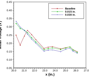
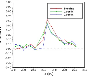
3.3 Mean Voltages

indicating that the length of the laminar separation bubble remains unchanged within the measurement resolution. The overall mean values decrease with increasing height, suggesting that the presence of the turbulator in this case has an adverse effect on the boundary layer flow.

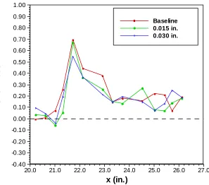
Similar results are observed for Case 2, Figure 3.7. The minimum mean voltages that are observed in the experimental data for the baseline case agree well with MSES predictions of the laminar separation and turbulent reattachment locations. A similar monotonic behavior is observed for the varying turbulator height, suggesting the turbulator has an adverse effect on the boundary layer flow for Case 2 as well. Overall, the mean values decrease as height of the turbulator increases, and neither separation nor reattachment locations are altered with deployment of the turbulator.

Case 4 has a laminar separation bubble that is comparable to that observed in Cases 1 and 2, Figure 3.9. The laminar separation and turbulent reattachment locations are confirmed with MSES results. When the turbulator is actuated, the mean voltages at which separation occurs increase in value. Although, the location of separation is not altered with actuation, the mean voltages increase in value indicating an increase in the local skin-friction. In addition, the smaller height appears to produce the more favorable flow as indicated by the overall highest mean voltages.

As a whole, the mean voltages measured from the baseline cases agree well with the theoretical separation and reattachment locations predicted by MSES. However, the deployment of the mechanical turbulator does not effectively eliminate or even reduce the laminar separation bubble, with the exception of Case 3. Only in two cases does the presence of the turbulator show favorable changes to the boundary layer flow.

closer the turbulator is located to laminar separation, the more effective the turbulator becomes. However, the effectiveness of turbulator height is not clearly seen in the present work.

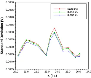
3.4 Standard Deviation

The standard deviation was calculated from high-pass filtered data to determine the point of transition and the effectiveness of the mechanical turbulator.

The standard deviation for the baseline of Case 1 is shown in Figure 3.10. A peak located at approximately 23.7-in downstream of the flat plate leading edge is considered to be the transition point. The theoretical result for Case 1 does not agree well with the maximum in the standard deviation. The presence of the turbulator can be seen, as the peak in standard deviation shifts upstream as the height of the turbulator is increased. This is observed for both heights, with transition occurring at approximately 23.2-in

downstream of the flat plate leading edge. Although the point of transition is not altered significantly, the mechanical turbulator does appear to cause the laminar flow to transition sooner. The effect of different heights is however is not seen in the standard deviation of Case 1.

location would be unchanged with the presence of the turbulator, which suggests the possible need for improved resolution of the hot-film sensor locations.

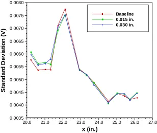
Similar results are obtained from the standard deviations calculated for Cases 3 and 4, Figures 3.12 and 3.13. The baseline cases show transition occurring at streamwise locations close to those predicted by MSES. Hot-film measurements of Case 3 show that transition occurs slightly upstream of that observed for the baseline case when the turbulator is actuated. The observed transition location is 0.3-in upstream of the baseline case. Case 4 shows no change in transition location when the mechanical turbulator is actuated.

3.5 Skewness

skewness is not as high as that observed for the baseline case. There is no clear effect of the height of the turbulator.

Case 3 exhibits yet another different trend than that observed in the skewness of the previous cases, Figure 3.16. The baseline shows a reversal in sign of the skewness. Upstream of separation the skewness in the baseline flow reaches a high positive peak of 0.55, and then decreases significantly until a negative skewness of –0.3 is reached. This reversal in sign is characteristic of transitional flow in an attached shear layer. In the present case of the unattached shear layer in the laminar separation bubble, the positive skewness extends over the upstream extent of the laminar separation bubble. The negative skewness occurs at a streamwise location immediately downstream of turbulent reattachment. The effect of the mechanical turbulator is to eliminate positive and negative peaks in skewness that are observed in the baseline flow. The skewness appears to level out and remains slightly positive for all streamwise locations.

Case 4 shows trends in the skewness that are similar to that seen in Case 2, with a high positive peak in the vicinity of the laminar separation bubble, Figure 3.17. The variation in the skewness remains relatively small outside of the laminar separation bubble.

3.6 Kurtosis

The kurtosis, also known as flatness, was calculated for all cases to determine the degree of nonlinear interactions in the laminar separation bubble. Generally, kurtosis has a value close to 3, for laminar and turbulent flows, while transitional flows have larger values different than 3.

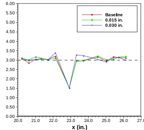
The kurtosis for Case 1 is shown in Figure 3.18. A large dip in the kurtosis is seen at 23-in, which is also the streamwise location where laminar separation was detected. This dip in the kurtosis exists for Case 1 with and without the turbulator, indicating that mechanical turbulators examined here have no effect on the kurtosis of Case 1. The kurtosis values upstream and downstream of this minimum suggest laminar flow upstream and turbulent flow downstream.

Case 2, Figure 3.19, shows a similar minimum in kurtosis at the same streamwise location, 23-in. This also corresponds to the location at which laminar separation is detected. The kurtosis rises above 3 downstream of separation and then returns to a relatively “flat” value near the location where turbulent reattachment is confirmed for Case 2. This correspondence with turbulent reattachment location is not seen in the kurtosis for Case 1. The kurtosis for Case 2 varies little with the turbulator.

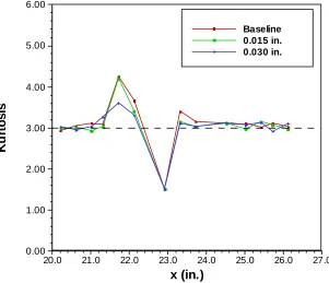
occurs further upstream near 21.0-in. More interesting is the pronounced effect of the turbulator, as the observed peak in the baseline case disappears. The kurtosis values with the turbulator remain very close to 3, indicating a smaller degree of nonlinearity in the flow. The effect of height of the turbulator is however not seen.

Case 4, Figure 3.21, shows a distribution of kurtosis that is similar to Case 2. The kurtosis increases above and then decreases below 3 over the region where the laminar separation bubble is observed. This is an indicator that a high degree of nonlinear interactions occur in the flow within the laminar bubble. The kurtosis values upstream and downstream of the bubble remain near values of 3, indicating laminar flow upstream and turbulent flow downstream. The effect of the height of the turbulator is not however clearly seen for Case 4.

Overall, the effect of the turbulator is not visible in the kurtosis of the hot-film signals, with the exception of Case 3, where the kurtosis remains near 3 when the turbulator is actuated. Kurtosis values above and below 3 are observed for all baseline cases in the region of the laminar separation bubble and are indicative of transitional flow.

3.7 Time Histories and Phase Reversal

The time histories are presented in Figures 3.22 to 3.30 for a 2-second long time segment. In part (a) of each plot the data from the seven downstream hot-film sensors are presented; in part (b) the data of the eight downstream sensors are presented. The data at

x=23.325-in are presented in both parts. For sake of clarity the time histories at each subsequent station are equally offset. Thus reading the data from bottom to top of the page presents the streamwise evolution of the flow. The time histories for the baseline of Case 1 are shown in Figure 3.22. Laminar separation was previously identified at 22.9-in; however, over the time segment presented here the 180o phase change is not clearly seen. It should however be noted that because of the problems with the data acquisition system the data from hot-film sensor number 13 (x=28.325-in) had to be disregarded. Perhaps if this time history signal were available, the phase change could be detected. A phase change in the vicinity of turbulent reattachment at x=25.7-in is not visible. The time history of Case 1 with a 0.030-in turbulator shows similar behavior to that observed in the baseline, Figure 3.23. However, the phase reversal highlighted with the oval symbol between the sensors located at 22.125-in and 22.925-in is observed, and the laminar separation is identified. A phase reversal is however not seen the region of turbulent reattachment.

with turbulator, Figure 3.25, shows similar results when compared to the baseline case as that seen in Case 1. The turbulator does not cause the laminar separation or turbulent reattachment points to change location, but more clearly shows the phase change.

The time history of Case 3, Figure 3.26, shows a clearly identifiable 180o phase change in the vicinity of 20.625-in, which corresponds to the laminar separation point previously detected at 20.6-in. Although not as clear, a phase change is seen between

x=22.925-in and 23.325-in. This agrees well to the turbulent reattachment location detected earlier at 22.9-in. The time histories of Case 3 with a mechanical turbulator are presented in Figure 3.27. A phase change is no longer seen between sensors in the vicinity of 20.625-in, nor in the region of the previously identified turbulent reattachment. A 180o phase change is however seen between x=21.025-in and 21.725-in, as well as between x=24.525-in and 25.025-in. It is uncertain what the nature of these phase reversals is for the case with turbulator, considering that neither laminar separation or turbulent reattachment are observed in the previous analysis of mean voltages. However, the results from MSES predict turbulent separation and turbulent reattachment, Figure 3.28, at these locations when the flow is transitioned at the turbulator.

does not appear have an effect on the laminar separation bubble, but merely makes more pronounced the presence of the separation and reattachment.

Overall, the observed 180o phase reversals in the time histories to determine laminar separation and turbulent reattachment locations agree well with the locations previously determined from the mean voltages. Case 3 is an exception as the identified separation and reattachment locations are not seen in the mean voltages, but agree with MSES predictions for a tripped flow.

3.8 Effects of Reynolds Number

The boundary layer thickness scales as an inverse power of Reynolds number, hence with increasing wind tunnel speed, the boundary layer thickness over the flat plate decreases. The boundary layer thickness at the location of the turbulator is calculated to be 0.119-in, 0.103-in, and 0.092-in, for the speeds of 30, 40, and 50ft/s respectively. For the largest turbulator height of 0.030-in at speeds of 30, 40, and 50ft/s, the height was 25, 29, and 33 percent, respectively, of the boundary layer thickness. It is thus of interest to see if the effectiveness of the mechanical turbulator is changed with Reynolds numbers. This was accomplished by examining the mean voltage and standard deviation of Case 4 at the three tunnel speeds with and without mechanical turbulator.

located at 21.3-in for speeds of 30 and 40ft/s. With an increase in speed to 50ft/s, the separation point moves upstream and is detected at 21.0-in. When the turbulator is actuated to a height of 0.015-in, the mean voltage increases for all speeds, Figure 3.32. Laminar separation remains at the same location as seen in the baseline for all speeds, but the trough created by the minimum mean voltage becomes shallower, creating a smoother mean voltage curve. At the larger height, 0.030-in, the effect of the turbulator appears most favorable for the higher tunnel speeds, Figure 3.33. A minimum in the mean voltage is not as apparent at a speed of 50ft/s, indicating that the laminar separation bubble is eliminated.

The standard deviation for Case 4 was analyzed at all speeds to determine the effect of the turbulator on the location of transition for the different Reynolds numbers. Figure 3.34 is the standard deviation for the baseline of Case 4 at 30, 40, and 50ft/s. As was previously determined, the peak in the standard deviation correlates well with the point of transition. In this case it is observed that the point of transition moves upstream with increasing wind tunnel speed. The location of transition is at 22.1-in, 21.7-in, and 21.3-in for speeds of 30, 40, and 50ft/s respectively. Tani4 also observed a similar movement in transition location with Reynolds number, as seen in Figure 3.35. In Tani’s work separation, transition, and reattachment location were measured on a circular cylinder and transition position were detected to move upstream with increasing Reynolds number, as is seen in the present experimental results.

however the peak in standard deviation is less pronounced as the measured standard deviation upstream of the transition location are increased.

At a turbulator height of 0.030-in, the standard deviation of Case 4 shows a change in transition location for a tunnel speed of 40ft/s, Figure 3.37. As seen previously, the presence of the mechanical turbulator causes the peak in the standard deviation to become more pronounced, as the transition location appears to move upstream. The transition location for 30 and 50ft/s remains the same as that observed for the baseline, however the transition point for 40ft/s appears to have moved upstream.

Overall, the effect of the mechanical turbulator is more clearly observed with the increase of Reynolds number. As the boundary layer thickness decreases with increasing Reynolds number, the percent height of the turbulator with respect to the boundary layer thickness increases to 33 percent. The more favorable results were obtained for the larger height at the larger Reynolds numbers, suggesting that if the heights of the turbulator selected for the present study may have been more effective if they were at heights more than 33 percent of the boundary layer thickness. However in a practical application the expected benefits of the larger heights would need to traded off against the parasite drag of the turbulator.

3.9 MSES Analysis with Forced Transition

forcing transition at the turbulator location, 18.75-in downstream of the flat plate leading edge. With transition occurring at this location, MSES predicts no laminar separation bubble for Cases 1, 2, and 4, Table 3.3. The predictions for Case 3 with forced transition produced an anomaly, which can not be clearly explained. Separation and reattachment are predicted to occur upstream of the location of the inverted airfoil, with streamwise locations of 14.3-in and 17.8-in respectively, Table 3.3. However, transition is predicted downstream of reattachment at 18.75-in, indicating the separated laminar boundary layer never transitions, which is uncharacteristic of a laminar separation bubble. Slightly downstream of transition, the boundary layer is predicted to separate once again at 20.1 -in and then reattach near 25.0-in downstream, creating a turbulent bubble.

CHAPTER 4

CONCLUDING REMARKS

4.1

Summary of Results

Experiments to determine the feasibility of using a mechanical turbulator to control on-demand in a predetermined manner the features of a laminar separation bubble have been conducted in the North Carolina State University Subsonic Wind Tunnel Facility. The tunnel is operated at speeds of 30, 40, and 50ft/s, with corresponding

freestream Reynolds numbers of 2.98×105, 3.97×105, and 4.97×105, based on the distance to the turbulator. The experimental set-up, based on the work of Gaster6, consists of a flat plate with an inverted airfoil mounted above its surface; the set-up allows laminar separation bubbles to be formed over a range of Reynolds numbers and pressure distributions.

An SMA-actuated mechanical turbulator that is capable of heights up to 0.040-in

Four test cases at a Reynolds number of 2.98×105 are examined with and without a turbulator. Statistical moments are computed from the time histories obtained from the hot-film sensors. These statistical moments include the mean, the standard deviation, the skewness, and the kurtosis. Minima in the mean voltage indicate separation and reattachment locations, and are in good agreement with the theoretical predictions. Peaks in the standard deviation of the high-pass filtered time traces agree well with the predicted transition locations. The skewness and kurtosis verify the regions of transitional flow within the laminar separation bubble. Low-pass filtered time traces of the hot-film signals are examined for 180o phase differences; this phase reversal is indicative of laminar separation and turbulent reattachment. Overall, the phase reversal, skewness, and kurtosis are not found to be as useful and reliable as the mean and standard deviation. Furthermore, as the latter two moments are easily calculated, they show promise for use in a real-time active flow control system.

More favorable results are obtained with the larger turbulator height at the larger Reynolds numbers; as the boundary layer thickness decreases with increasing Reynolds number, the relative height of the turbulator with respect to the boundary layer thickness increases to 33 percent. The heights examined in the present study were calculated based on minimum turbulator height necessary to cause transition over the airfoil of a sailplane.16 This suggests that such practical turbulator heights, as examined in the present study, are not suitable for predetermined control of the laminar separation bubble. This range of turbulator heights neither makes the flow more unstable nor trip the flow at the location of the turbulator. For transition occurring at the location of the turbulator, MSES predicts that no laminar separation bubble is formed. Therefore, there is perhaps a critical turbulator height above which transition will occur at the location of the turbulator. However, in a practical application, the benefits of eliminating the laminar separation bubble must be traded off against the added turbulent skin friction and parasite drag.

gradient is absent. This set-up thus allows the effects of the turbulator on the laminar separation bubble to be more clearly identified.

In conclusion, for the range of turbulator heights examined, the adaptive mechanical turbulator is not suited to provide proportional control of a laminar separation bubble. No monotonic variation of the locations of separation, transition, or reattachment is observed with varying turbulator height. This in turn suggests that there is perhaps a critical turbulator height above which transition will occur at the turbulator location.

4.2

Recommendations for Future Work

CHAPTER 5

REFERENCES

1. Mueller, T. J., “Low Reynolds Number Vehicles,” AG-288, AGARD, 1985. 2. Greer, D., and Hamory, P., “Design and Predictions for High-Altitude (Low

Reynolds Number) Aerodynamic Flight Experiment,” Journal of Aircraft, Vol. 37, Number 4, July-August 2000, pp. 684-689.

3. Gad-el-Hak, M., Flow Control: Passive, Active, and Reactive Flow Management, Cambridge University Press, New York, 2000, pp. 189-204.

4. Tani, I., “Low-Speed Flows Involving Bubble Separations,” Progress in Aeronautical Sciences, Vol.5, 1964, pp. 70-103.

5. Dovgal, A. V., Kozlov, V. V., and Michalke, A., “Laminar Boundary Layer Separation: Instability and Associated Phenomena,” Progress in Aerospace Sciences, Vol. 30, 1994, pp. 61-94.

6. Gaster, M., “The Structure and Behaviour of Separation Bubbles,” Aeronautical Research Council R. & M. 3595, 1969.

7. Ward, J. W., “Behaviour and Effects of Laminar Separation Bubbles on Aerofoils in Incompressible Flow,” Journal of the Royal Aeronautical Society, Vol. 67, December 1963, pp. 783-790.

8. Mueller, T. J., and Batill, S. M., “Experimental Studies of Separation on a Two-Dimensional Airfoil at Low Reynolds Numbers,” AIAA Journal, Vol. 20, Number 4, April 1982, pp. 457-463.

9. Liebeck, R. H., “Laminar Separation Bubbles and Airfoil Design at Low Reynolds Numbers,” AIAA Paper 92-2735-CP, 1992.

10. Lin, J. C. M. and Pauley, L. L., “Low-Reynolds-Number Separation on an Airfoil,” AIAA Journal, Vol. 34, Number 8, August 1996, pp. 1570-1577.

11. Vatsa V. N., and Carter, J. E., “Analysis of Airfoil Leading-Edge Separation Bubbles,” AIAA Journal, Vol. 22, Number 12, December 1984, pp. 1697-1704. 12. Drela, M., and Giles, M. B., “Viscous-Inviscid Analysis of Transonic and Low

13. Maughmer, M. D., and Somers, D. M., “Design and Experimental Results for a High-Altitude, Long-Endurance Airfoil,” Journal of Aircraft, Vol. 26, Number 2, February 1989, pp. 148-153.

14. Selig, M. S., Gopalarathnam, A., Giguère, P., and Lyon, C., “Systematic Airfoil Design Studies at Low Reynolds Numbers,” Presented at the conference on Fixed, Flapping and Rotary Wing Vehicles at Very Low Reynolds Numbers, Notre Dame, IN, June 5 – 7, 2000.

15. Lyon, C., Selig, M., and Broeren, A., “Boundary Layer Trips on Airfoils at Low Reynolds Numbers,” AIAA Paper 97-0511, January 1997.

16. Johnson, R. H., “Are Your Turbulators Too Large?,” Soaring Magazine, January 1995, pp. 29-31.

17. Kral, L. D., “Active Flow Control Technology”, ASME Fluids Engineering Division Technical Briefing, 1999.

18. “Materials for Smart Systems,” Proceedings of Materials Research Society Symposia, Vol. 360. George, E. P. (Ed.) Materials Research Society, Pittsburgh, PA, 1995.

19. Bellhouse, B. J., and Schultz, D. L., “Determination of Mean and Dynamic Skin Friction, Separation and Transition on Low-Speed Flow with a Thin-Film Heated Element,” Journal of Fluid Mechanics, Vol. 24, Part 2, 1966, pp. 379-400.

20. Menendez, A. N., and Ramaprian, B. R., “The Use of Flush-Mounted Hot-Film Gauges to Measure Skin Friction in Unsteady Boundary Layers,” Journal of Fluid Mechanics, Vol. 161, 1985, pp. 139-159.

21. Stack, J. P., Mangalam, S. M., and Berry, S. A., “A Unique Measurement Technique to Study Laminar-Separation Bubble Characteristics on an Airfoil,” AIAA Paper 87-1271, June 1987.

22. Stack, J. P., Mangalam, S. M., and Kalburgi, V., “The Phase Reversal Phenomenon at Flow Separation and Reattachment,” AIAA Paper 88-0408, January 1988.

23. Mangalam, S. M., Sewall, W. G., Stack, J. P., and McGhee, R. J., “A New Multipoint Thin-Film Diagnostic Technique for Fluid Dynamic Studies,” SAE Paper 881453, October 1988.

25. Sarma, G. R., U.S. Patent No. 5,074,147, 1991.

26. Sarma, G. R., “Transfer Function of the Constant Voltage Anemometer,” Review of Scientific Instruments, Vol. 69, Number 6, June 1998, pp. 2385-2391.

27. Bertelrud, A., “Transit ion on a Three-Element High Lift Configuration at High Reynolds Numbers,” AIAA Paper 98-0703, January 1998.

28. Chokani, N., “Nonlinear Spectral Dynamics of Hypersonic Laminar Boundary Layer Flow,” Physics of Fluids, Vol. 11, Number 12, December 1999.

29. Drela, M., “Newton Solution of Coupled Viscous/Inviscid Multielement Airfoil Flows,” AIAA Paper 90-1470, June 1990.

30. Evangelista, R., McGhee, R., and Walker, B., “Correlation of Theory to Wind Tunnel Data at Reynolds Numbers Below 500,000,” Paper presented at Conference on Low Reynolds Number Aerodynamics, University of Notre Dame, Indiana, June 1989.

31. Walker, G. J., “Transitional Flow on Axial Turbomachine Blading,” AIAA Journal, Vol. 27, Number 5, May 1989, pp. 595-602.

CHAPTER 6

49

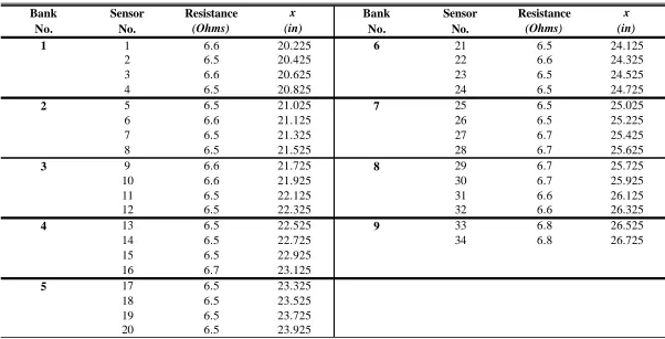
Table 2.1 – Sensor resistance and location (inches).

Bank Sensor Resistance x Bank Sensor Resistance x

No. No. (Ohms) (in) No. No. (Ohms) (in)

1 1 6.6 20.225 6 21 6.5 24.125

2 6.5 20.425 22 6.6 24.325

3 6.6 20.625 23 6.5 24.525

4 6.5 20.825 24 6.5 24.725

2 5 6.5 21.025 7 25 6.5 25.025

6 6.6 21.125 26 6.5 25.225

7 6.5 21.325 27 6.7 25.425

8 6.5 21.525 28 6.7 25.625

3 9 6.6 21.725 8 29 6.7 25.725

10 6.6 21.925 30 6.7 25.925

11 6.5 22.125 31 6.6 26.125

12 6.5 22.325 32 6.6 26.325

4 13 6.5 22.525 9 33 6.8 26.525

14 6.5 22.725 34 6.8 26.725

15 6.5 22.925

16 6.7 23.125

5 17 6.5 23.325

18 6.5 23.525

19 6.5 23.725

Table 3.1 – Experimental test cases selected for analysis.

Airfoil Height Airfoil Angle Airfoil Streamwise Location Case (Airfoil Leading Edge of Attack ( Airfoil Leading Edge Number to Flat Plate) (degrees) to Flat Plate Leading Edge)

(in.) (in.)

1 1.875 5.0 20.0

2 0.9375 0.0 20.0

3 0.9375 0.0 17.563