Study of a low Re airfoil considering laminar separation bubbles in static and pitching motion

(1)

Study of a low Re airfoil considering

laminar separation bubbles in static

and pitching motion

by

Faegheh Ghorbanishohrat

A thesis

presented to the University of Waterloo in fulfillment of the

thesis requirement for the degree of Doctor of Philosophy

in

Mechanical and Mechatronics Engineering

Waterloo, Ontario, Canada, 2019

c

(2)

Examining Committee Membership

The following served on the Examining Committee for this thesis. The decision of the Examining Committee is by majority vote.

External Examiner Pierre Sullivan

Professor, Dept. of Mechanical & Industrial Engineering, University of Toronto

Supervisor David Johnson

Professor, Dept. of Mechanical & Mechatronics Engineering, University of Waterloo

Internal Member Carolyn Ren

Internal Member Xianguo Li

Internal-external Member Ali Elkamel

Professor, Dept. of Chemical Engineering, University of Waterloo

(3)

I hereby declare that I am the sole author of this thesis. This is a true copy of the thesis, including any required final revisions, as accepted by my examiners.

(4)

Abstract

Performance of low Reynolds number (Re) devices is highly dependent on their airfoil design. Small wind turbines that usually work in areas with poor wind resources with a vast application from remote to busy urban regions are no exception. The unsteady flow field around the turbine blade results in an unsteady boundary layer that makes aerodynamics of these turbines complex and interesting. But due to the complexity of unsteady low Reynolds flow, and the small scale of boundary layer flow there are still unanswered questions in this area. Therefore, this study is arranged to fully investigate low Reynolds number boundary layer flow in steady and unsteady flow using small scale experiments.

For this goal, three non-intrusive experimental techniques used to study low Re flow behavior over a miniature SD7037 airfoil including surface oil flow visualization (SOFV), IR-Thermography (IT), and particle image velocimetry (PIV) at 14000≤Re≤48000 have been developed and utilized. To model unsteady flow a pitch oscillation about the static stall angle of attack with amplitude 9◦ was considered. The quality of acquired results from all the experimental methods confirms the possibility of downscaling of low Reynolds flow experiments. Flow parameters such as the separation and reattachment points were quantitatively determined from SOFV and IT. The high-resolution PIV measurements provided an accurate velocity field so that surface pressure distribution and estimation of skin friction coefficient were determined from the velocity fields in both the steady and unsteady flow where due to the scale of the experiment and low magnitude of shear stress other measurement techniques would be intrusive or cannot be used. Estimated surface pressure coefficient (Cp) from PIV data revealed vortical structure effects as low-pressure waves that cannot be captured with coarse resolution methods. Integral boundary layer parameters are calculated in steady and unsteady conditions that provide in-depth information regarding low Re boundary layer flow behavior and laminar separation bubble characteristics. Boundary layer flow and reversed flow under the separated bubble were captured precisely while the Field of View covers the whole airfoil and results were confirmed by acquired data using finer spatial resolution. The measured aerodynamic force shows the effect of the height of the bubble on increasing the drag and the proper orthogonal decomposition method provided more information regarding the time-dependent behavior of vortices.

(5)

Acknowledgements

The beginning of my Ph.D. program was associated with a significant change in my life as starting to live in a new country, far from my family and friends. From that day many people helped me during this journey that without them this would not have been possible.

First and foremost, I would like to thank and express my special appreciation to my supervisor, Professor David Johnson who made this work possible. I would like to thank him for giving me the opportunity to work on this fascinating project and so selflessly and passionately mentored and guided me throughout my Ph.D. studies and shared his immense knowledge with me. He has been a tremendous mentor for me who helped me to overcome the difficult times and to stay positive in my work and my personal life.

I would also like to say special thanks to my Ph.D. committee members, Professors Pierre Sullivan, Carolyn Ren, Ali Elkamel, and Xianguo Li for their support and guidance.

I would also like to thank University of Waterloo faculty members, staff, and technicians especially Jason Benninger who helped with all the lab related challenges and Martha Morales.

During my studies, I met wonderful colleagues and friends who without them life would not have been as lovely. So many thanks to Nicholas Tam, Kobra Gharali, Nigel Swytink-Binnema, Farid Samara, Alison Zilstra, Micheal McKinnon, Michel Gaetan, Rifki Nugroho, and Mehrdad Bakhtiari for their help and support. I would also like to thank all our co-op students.

Finally, I want to show my deepest love to my amazing family; my parents Azar and Mohsen, my siblings and in-laws Fakhteh, Adele, and Fariborz who supported me during the hardest times of my life and gave me hope, joy, and courage to complete my studies. My nephew, Farbod who his smile warms my heart. And Nima, for his love and support. He never let me feel alone and encouraged me to pass all obstacles and appreciate every day of my life as an opportunity to learn.

(6)

Dedication

(7)

List of Tables

3.1 Statistical uncertainty for PIV method, Re=41000 . . . 53

4.1 Static case studies. . . 84

4.2 Summary of various methods to characterize LSB used in this thesis . . . . 85

4.3 Laminar separation bubble parameters for investigated static cases using Cp 94

4.4 Laminar separation bubble parameters for static cases using Cf . . . 102 4.5 Laminar separation bubble parameters for static cases using integral BL

features . . . 109

5.1 Dynamic case studies . . . 126

(11)

List of Figures

1.1 Aerodynamic efficiency at different Re . . . 2

1.2 Aerodynamic sources affecting wind turbine airloads . . . 3

1.3 Velocity and pressure distribution in the Bl. . . 5

1.4 BL flow behavior on flat plate at zero incidence . . . 6

1.5 Schematic of laminar separation bubble . . . 8

1.6 Airfoil unsteady aerodynamic models (pitch and plunge) . . . 10

1.7 Surface pressure distribution in existence of LSB . . . 14

1.8 Streamwise velocity fluctuations over 2D OA209 helicopter fan blade . . . 16

1.9 Cat-eye pattern in Kelvin-Helmholtz instabilities. . . 18

1.10 Pressure coefficient distribution over NACA-0015 at pitch up motion . . . 23

1.11 Surface pressure distribution over a bionic airfoil at AOA=0◦ . . . 23

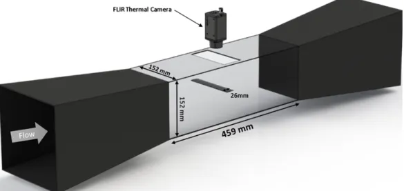
2.1 Test section side view and schematic of wind tunnel . . . 30

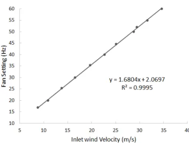
2.2 Inlet wind velocity and temperature versus VFD fan setting (Hz) . . . 31

2.3 Schematic of the SD7037 airfoil compared with NACA0012. . . 31

2.4 Manufactured SD7037 airfoil model . . . 32

2.5 Servomotor in addition to the coupling and model . . . 33

2.6 Oil flow visualization setup . . . 35

2.7 Surface oil flow visulaization samples . . . 36

2.8 Schematic of wind tunnel and IT thermal camera experimental setup. . . . 38

(12)

2.10 A schematic of experimental setup. . . 39

2.11 Experimental setup with size details. . . 40

2.12 PIV technique . . . 40

2.13 The effect of different power in dual pulse laser . . . 41

2.14 Sample PIV image . . . 43

2.15 PIV images FOVs . . . 44

2.16 Adjusted calibration device. . . 45

2.17 Example of program application . . . 46

3.1 Comparison of the cross-correlation at different locations . . . 49

3.2 Interrogation area overlapping . . . 50

3.3 Sample IAs from different parts of an image . . . 53

3.4 Sample PIV result of FOV=2.5c- case Re=40,000, AOA= 7◦ . . . 55

3.5 Sample PIV result of FOV=c- case Re=40,000, AOA = 7◦ . . . 56

3.6 Sample PIV result of FOV=0.6c- case Re=40,000, AOA= 7◦ . . . 57

3.7 Detection of flow regions from raw PIV image . . . 58

3.8 Mean streamwise velocity component(Us) . . . 58

3.9 Detection of the separation point . . . 59

3.10 Detection of the LSB’s height . . . 59

3.11 Detection of the BL Profile. . . 61

3.12 BL quantities in the existence of the LSB . . . 62

3.13 Sample measured BL quantities in the existence of the LSB. . . 62

3.14 Surface pressure coefficient over SD7037 airfoil . . . 64

3.15 Skin friction coefficient over SD7037 airfoil . . . 65

3.16 Profile of the LSB . . . 66

3.17 Schematic showing the control volume used for the 2D momentum theory . 68 3.18 Schematic showing the two different methods the pressure field is calculated for the different regions of the flow. . . 70

(13)

4.1 Location of separation and reattachment points vs angles of attack . . . . 72

4.2 Surface oil flow visualization for Re= 48000 and 32000 . . . 74

4.3 Position of separation and reattachment points vs Re . . . 75

4.4 Changes of the length of the LSB by changing α and Re . . . 76

4.5 Thermographic flow visualization with air heater at 4◦ and 7◦ . . . 77

4.6 Thermographic flow visualization with air heater at 10◦, 11◦ . . . 78

4.7 Thermographic result of air heater method at 10◦, 11◦ . . . 79

4.8 Thermographic flow visualization with electrically conductive paint . . . . 81

4.9 Thermographic flow visualization resistant heating wire method at 1◦ and 7◦ 82 4.10 Separation and reattachment locations for SOFV and IT . . . 83

4.11 S-N coordinates Over SD7037C Airfoil . . . 84

4.12 Comparison of pressure distribution over SD7037 airfoil for different Ncrit in XFoil . . . 87

4.13 Lift coefficent (Cl) of SD7037 airfoil at Re=60,000 . . . 87

4.14 Pressure distribution over SD7037 airfoil, case Re=40,000,AOA = 1◦ . . . 88

4.15 Pressure distribution over SD7037 airfoil, case Re=40,000,AOA = 5◦ . . . 89

4.16 Comparison of Cp over SD7037 airfoil at Re=41,000 (PIV experimental results and XFoil) . . . 89

4.17 Comparison of Cp over SD7037 airfoil at Re=32000, and 48,000 (PIV experi-mental results and XFoil) . . . 90

4.18 Pressure distribution over the suction side of SD7037 airfoil at Re=48000 measured from PIV data . . . 91

(14)

4.23 Surface Pressure Coefficent over SD7037 airfoil at AOA=3◦ and 5◦ at all investigated Re. . . 95

4.24 Surface Pressure Coefficent over SD7037 airfoil at AOA=7◦ and 9◦ at all investigated Re. . . 96

4.25 Instantaneous velocity field, SD7037 airfoil, case Re=14000, AOA=5◦ . . . 96

4.26 Instantaneous velocity field, SD7037 airfoil, case Re=22000, AOA=5◦ . . . 97

4.27 Time averaged velocity field over SD7037 airfoil, Re=14000, AOA=5◦ . . . 97

4.28 Time averaged velocity field over SD7037 airfoil, Re=22000, AOA=5◦ . . . 98

4.29 Transition ramp on SD7037 airfoil at Re=41000, AOA=7◦ . . . 99

4.30 Surface oil flow visualization over SD7037 airfoil, Re=32000, AOA=9◦ . . . 99

4.31 Time averaged velocity vectors, SD7037 airfoil, case: Re=32000, AOA=9◦ . 100

4.32 Skin friction coefficient distribution over the upper surface of SD7037 airfoil 101

4.33 Instantaneous and time averaged normal velocity component contour over SD7037 airfoil, case Re=32000,AOA= 5◦ . . . 103

4.34 Shape Factor H vs X/C, SD7037 airfoil, Re=48000, AOA=3◦, 5◦, 7◦, 9◦ . . 105

4.35 Shape factor H at different AOA and Re . . . 106

4.36 δ∗ over SD7037 airfoil at Re=48,000. . . 108

4.37 δ∗ and θ versus X/C, SD7037 airfoil at Re=41,000 . . . 108

4.38 Velocity contours and velocity vectors vs X/C, SD7037 airfoil, Re=41000, AOA=9◦ . . . 111

4.39 A schematic of the process of instabilities and transition from laminar to turbulent flow . . . 111

4.40 Velocity Fluctuation profiles versus X/C, SD7037 airfoil, case Re=48000,AOA= 7◦ . . . 112

4.41 Velocity fluctuations vectors (

√

u02 U2_∞,

√

v02

U2_∞) over SD7037 airfoil, case: Re=41000, AOA=9◦ . . . 112

4.42 Time averaged velocity contour and velocity vectors at Re=22000 to 48000 at AOA=5◦ over SD7037 airfoil . . . 114

4.43 Time averaged velocity contour and velocity vectors at Re=22000 to 48000 at AOA=9◦ over SD7037 airfoil . . . 115

(15)

4.44 Sample FOV of POD analysis . . . 117

4.45 Instantaneous streamlines and velocity field over the airfoil at Re=41000 and AOA of 5◦ . . . 117

4.46 Streamlines of averaging of 300 analyzed pair images at Re=41000 and AOA of 5◦ . . . 118

4.47 Covariance and Velocity streamlines over SD7037 airfoil at Re=32000 and AOA 5◦ . . . 119

4.48 Average of streamwise velocity component (u) along BL velocity profiles and contour of Reynolds shear stress at Re=32000 and AOA 5◦.. . . 119

4.49 Modal energy distribution of velocity vector (u,v) for different sample size, Re=32000 and AOA 5◦ . . . 120

4.50 Projection of POD modes 1 and 2 of the velocity component of v (airfoil is white) . . . 121

4.51 A time history of POD coefficient values for modes 1 and phase portrait of modes 1 and 2 at Re= 3×104 _{and AOA 5}◦_. _{. . . .} ₁₂₂

4.52 Modal energy distribution for velocity vector (u,v), Re=41000 . . . 123

4.53 First 6 modes of velocity componentv, andu, Re=41000 and AOA 5◦. . . 124

5.1 Pressure distribution over the suction side of SD7037 airfoil at Re=41000, k=0.1 measured from PIV data . . . 127

5.4 Effects of the reduced frequency on measured surface pressure distribution over SD7037 airfoil at Re=41,000 . . . 129

5.5 Tangential velocity component contour over SD7037 airfoil at Re=41,000, AOA=9◦ at k=0, 0.05,0.08, and 0.10 . . . 131

5.6 Normal velocity component contour over SD7037 airfoil at Re=41,000, AOA=9◦ at K=0, 0.05,0.08, and 0.10 . . . 131

5.7 Tangential velocity component contour over SD7037 airfoil, case: Re=41,000, AOA=11◦, k=0.05, 0.08, 0.10 . . . 132

(16)

5.8 Normal velocity component contour over SD7037 airfoil, Re=41,000, AOA=11◦,

k=0.05, 0.08, 0.10 . . . 133

5.9 Tangential velocity component contour over SD7037 airfoil, Re=22,000, AOA=12◦, k=0.10 . . . 134

5.10 Normal velocity component contour versus X/C, SD7037 airfoil, Re=22,000, AOA=12◦, 13◦, k=0.10 . . . 135

5.11 Pressure distribution over the suction side of SD7037 airfoil at Re=22000, k=0.05 measured from PIV data. . . 136

5.12 vorticity (ωz) and u0v0(m/s)2 fields about SD7037 airfoil at Re=22000, k=0.1137 5.13 Instantaneous and time averaged velocity contour, SD7037 airfoil, Re=41000, k=0.08, AOA= 9◦ . . . 139

5.14 Instantaneous and time averaged velocity contour, SD7037 airfoil, Re=32000, k=0.08, AOA= 9◦ . . . 140

5.15 Skin friction coefficient distribution over the upper surface of SD7037 airfoil, case: Re=32000, k=0.08 . . . 141

5.16 ∂us_∂y versus X/C, SD7037 airfoil, case: Re=32000, k=0.08, AOA=7◦ . . . 142

5.17 ∂us_∂y versus X/C, SD7037 airfoil, case: Re=32000, k=0.08, AOA=9◦ . . . 142

5.18 Shape Factor H, SD7037 airfoil, k=0.05, Re=41000, AOA=5◦-11◦ . . . 144

5.19 δ∗, SD7037 airfoil, k=0.05, Re=41000, AOA=5◦-11◦ . . . 144

5.20 Transition point location versus X/C, SD7037 airfoil, Case: k=0.05, Re=41000, AOA=5◦-11◦ . . . 145

5.21 Lift and drag coefficients versus AOA, SD7037 airfoil . . . 146

(17)

Nomenclature

A Axial Force [N].

Aspan Span area of airfoil [m2].

b Span length[m]. c Chord length [m]. CD Drag coefficient. CL Lift coefficient. Cp Pressure coefficient. D Drag Force [N]. f Frequency of Oscillation [Hz]. fv Frequency of Vortex shedding [Hz].

H Boundary layer shape factor. hb Bubble Height[m].

k Reduced Frequency. L Lift Force [N]. lb Bubble length[m].

N Direction Normal to the Surface. n Number of Refinement Steps. p Precision uncertainty.

Patm Atmospheric pressure [Pa].

Re Strouhal number. St Reynolds number.

Ue Streamwise velocity at the edge of the

bound-ary layer[m/s].

U∞ Free Speed Velocity [m/s].

utot Total uncertainty.

xR, R Reattachment point[m].

xs, S Separation point[m].

(18)

α Angle of attack [◦].

αamp Pitch Oscillation Amplitude [◦].

αmean Mean angle of attack [◦].

δ Boundary Layer thickness[m]. δ∗ Displacement thickness[m]. µ Dynamic Viscosity [kg/m s]. ν Kinematic Viscosity [m2_/s]. λ Wave Length[m].

ρ Density [kg/m3_]. τ Shear Stress [Pa]. τw Wall Shear Stress [Pa].

σ Standard deviation. θ Momentum thickness[m]. 2D Two Dimensional.

3D Three Dimensional. AOA Angle of Attack.

CF D Computational Fluid Dynamics. DAQ Data Acquisition.

DOF Degree of Freedom. F OV Field of View.

HAW T Horizontal Axis Wind Turbine. LE Leading Edge.

M AV Micro Air Vehicle. N I National Instruments. SW T Small Wind Turbine. T I Turbulent Intensity. T E Trailing Edge.

U AV Unmanned Aerial Vehicle. U W University of Waterloo. W T Wind Turbine.

(19)

Chapter 1 Introduction

Aerodynamic efficiency increases dramatically in the transitional Reynolds number(Re) region (104_-106_)[₈₆_, ₁₀₉_{]. Figure} _1.1_{shows the trend of aerodynamic efficiency versus Re.} Applications such as Micro Air Vehicles (MAV), Unmanned Aerial Vehicles (UAV), and Small Horizontal Axis Wind Turbines (SWT) typically operate in this low Re regime. Due to significant progress in technology, an increase in their performance and efficiency is considered much more than before.

SWTs are one of the sources of green energy that can be used from the most populated cities to totally remote regions that makes them one of the areas of interest in research. SWTs are designed to operate individually at lower local wind speeds, and then their efficiency becomes relatively more important compared to large commercial wind turbines. One of the most important components of a wind turbine which has a great effect on the efficiency is the blade. Therefore, the design of the blade becomes a crucial part of the strategy to maximize the efficiency of wind turbines especially for SWTs. However, wind turbine aerodynamics are complex due to many reasons including unsteadiness. For this reason unsteady blade air loads, blade performance, aeroelastic response of the blade, and environmental effects such as ground boundary layer effects should be considered all together[71]. The unsteady flow field around the turbine blade can cause an unsteady boundary layer (BL) which is affected by parameters such as environmental conditions, size of the blade (i.e., aeroelastic effect), and wind velocity.

Other low Re devices such as UAVs, MAVs, and low-pressure turbine blades operate under similar conditions. Poor aerodynamic performance for MAVs working at Re less than 70,000 was reported to be partly due to airfoil performance[112]. At low Re, a thick boundary layer increases the viscous drag [112] and formation of a laminar separation

(20)

Figure 1.1: Aerodynamic efficiency vs. chord Re[109,86]

bubble on the suction side of the airfoil increases the pressure drag [132] that results in a considerable drop in performance.

In summary, in low Re flows transition occurs and can include a laminar separation bubble (LSB). Formation of the LSB over the airfoil and sensitivity of this phenomenon to parameters such as the angle of attack (AOA), turbulence intensity (TI), and Re could cause unexpected behavior in aerodynamic forces followed by undesired changes in airfoil performance. In order to design an optimum airfoil and achieve better performance in low Re applications, further understanding of flow behavior and especially the laminar separation bubble on a low Re airfoil in different static and dynamic conditions is necessary and will be the subject of this study.

1.1 Low Re applications and small-scale experiments

Small Horizontal Axis Wind Turbines Wind turbines are devices which convert kinetic energy from the wind usually into electrical power. SWTs are used for many different applications such as remote off-grid residences and farms, telecommunication towers, offshore platforms and boats to name a few and are designed to operate at lower wind speeds. Therefore, regarding the increased concern about the use of green energy in the world, SWTs can potentially be one the major sources of energy for urban and rural life.

SWTs can include micro turbines rated less than 5kW, residential applications, 1kW to 10kW, and farm or institutional uses more than 10kW up to 300kW with a typical total

(21)

Figure 1.2: Aerodynamic sources affecting wind turbine airloads

height for a small horizontal wind turbine rated at 250kW is about 75m[105]. Loads on SWTs are typically controlled through stall-regulation, meaning that with an increasing wind velocity higher than a certain value, the blade surface area covered by separated flow increases, and eventually, the wind turbine captures less energy than before. This passive control method decreases the cost of small wind turbines but makes these turbines highly dependant on the aerodynamic design of the blade. Wind turbines usually operate under dusty weather conditions; therefore, the turbine blade erodes with undesirable roughness. Due to the cold weather in some parts of Canada, ice can develop on the leading edge (LE) of the blade which changes the effective shape of the LE and surface roughness. Roughness variation due to the conditions such as ice-covering of the blade can make changes occur in the airfoil laminar separation and turbulent transition phenomena[121] which can cause a reduction in the airfoil performance and captured energy. Therefore, sensitivity to roughness should be reduced[105, 118]. Wind turbines, due to the working environment, experience unsteady conditions. Figure1.2, shows a summary of aerodynamic sources presented by Leishman[71] that can affect wind turbine blade loads.

Some prior scaled wind turbine experiments have Re in the order of 103 _{to 10}4_{, based on} tip section of the blade[87]. For small wind turbines increasing the performance also depends to the response of SWTs to low startup wind speeds that could be about 3-8m/s[125].

Micro Air Vehicles MAVs are getting more attention in the market and typical airfoils for these applications are in the Re range from 103 to 105. Thin airfoils with camber up to 8% that provide higher performance in lower Re are reported for these application[112].

This study covers the Re range of 1.5×104 _{to 5}_×₁₀4 _{to study boundary layer flow in} static and pitching motion over a low Re airfoil . The next section provides a short theory of boundary layer and laminar-turbulent transition.

(22)

1.2 Theory

1.2.1 Boundary-Layer

An object in a flow is subjected to two types of forces, normal and tangential forces. One tangential force, the friction force (friction drag) is related to the fluid viscosity, where the viscosity highly depends on the fluid temperature. The effects of viscosity are considerable in a narrow region in the vicinity of a wall, as the velocity grows from zero on the wall to the free stream velocity and this region is called the Boundary Layer. Apart from this region, the flow may treated as inviscid. Although the boundary between these two regions is not clear, particularly in laminar flows, where the velocity reaches the 99% of free stream velocity is considered to be the boundary. Regarding equation 1.1 shear stress and its resulting friction drag have an inverse relation with boundary layer thickness[111]. Laminar wall shear stressτw is typically written as:

τw(x) =µ(

∂u

∂y)w (1.1)

where µ is the viscosity, y is the direction perpendicular to the surface and u is the velocity. In inviscid flow, the outer region, the pressure distribution changes along the surface geometry and this pressure imposes onto the limit of the BL. In the narrow BL region, the pressure is constant perpendicular to the wall. Simplistically, while particles in both regions are under the same pressure distribution, in the BL due to the friction force particles lose kinetic energy and may flow toward a higher pressure and as a result may divert to the main flow leading to flow separation from the surface and a separated shear layer[63, 92]. Accordingly, the separation point is the junction of forward flow and reverse flow. The slope of the velocity profile at the separation point at the wall is zero (∂u_∂y = 0 at y= 0). Representative velocity profiles are shown in Figure1.3.

Before the separation point, there is an accelerated BL flow with a favorable pressure gradient (dp_dx <0). Simplifying the boundary layer equation 1.2(simplified Navier-Stokes momentum equation in the boundary layer) on the wall ((u, v)w = (0,0)) reveals (∂

2_u ∂y2)<0

in the viscous layer before separation.

u∂u ∂x +v ∂u ∂y =− 1 ρ dp dx +ν ∂2u ∂y2 (1.2)

After the separation point, the flow has an adverse pressure gradient (dp_dx > 0) that means (∂_∂y2u2)w > 0. Further along the BL far from the separated shear layer, (∂

2_u ∂y2) < 0,

(23)

PI Xs y y U y y y U y (a) a) (b) b) x y

Figure 1.3: Velocity distribution in the BL a) favorable pressure gradient b) adverse pressure gradient

therefore somewhere in the middle (∂_∂y2u2) = 0. This point is the point of inflection (PI) of

the velocity profile[111]. This is a sufficient condition for amplified disturbances to develop inviscid flow instability(Kelvin- Helmholtz)[12, 25]. Figure 1.3 shows a velocity profile in the BL with its first and second derivatives profiles.

1.2.2 Instability and Transition

BL flows can be laminar if flow particles move in layers without strong exchange between layers, or it can be turbulent if particles move in irregular and random behaviour in both time and space which causes significant particle transfer between layers. In turbulent flow, effects of viscosity are limited in a narrow layer on the wall that is called the viscous or laminar sublayer where the velocity gradient is very large. Laminar flow transitions to turbulent flow with random fluctuating motions. It occurs when small 2D perturbations, Tollmien-Schlichting (T-S) waves caused by wall roughness or outer flow irregularities appear in laminar BL flow, and the viscosity is not enough to dampen them. These disturbances grow and intensify to a 3D disturbance that characterizes turbulent flow. For lower Re flows even small perturbations can destabilize the BL while with increasing Re the laminar BL is more stable [111]. Figure1.4 is a schematic of the transition process in a laminar BL

(24)

Figure 1.4: BL flow behavior on flat plate at zero incidence.[111, 134]

flow on a flat plate. As shown, following stable laminar flow (1) the transition region begins with initiating unstable 2D Tollmien-Schlichting (T-S) waves(2) moving downstream, and they become elongated to span-wise vortices and form a Λ structure vortex (3), following by 3D vortex breakdown(4) and a turbulent flow region(5)[35, 111].

When transition phenomenon occurs in the separated shear layer, disturbances due to T-S instabilities roll up into vortices along the span. Downstream, merging and break down of these vortices causes mixing of the layers and increases the flow momentum. If the energy of the flow is large enough, the separated shear layer reattaches to the surface as turbulent flow and forms a Laminar Separation bubble (LSB)[35,63, 108]. Although the creation of a LSB may prevent the airfoil from stalling, vortices formed along with the LSB can increase the noise level and/or fluctuating load on the airfoil[63].

Although the BL region is a narrow area, its impact on airfoil performance is significant so that forces acting on the body are highly dependent on the type of BL[111]. Therefore, more understanding of laminar BL transition and its affecting parameters such as vortices could help in developing low-Re applications.

1.2.3 Laminar Separation Bubble (LSB)

In many applications that deal with low Reynolds number flows (1×104 to 50×104)[53], such as turbomachinery, unmanned aerial vehicles, micro air vehicles, and wind turbines, smooth transition1 _{occurs with the existence of a LSB. For example, SWTs usually work}

in areas with a poor wind resource and they face continuous changes in wind speed and

(25)

direction. Therefore, a large part of the SWTs’ blade operates under laminar or transitional flow [79]. Shear stress and heat transfer rate increases in transition which both can have effects on the drag force[28], the rate of increase or decrease of these features can be used to define or aid in interpretation of experiments. Therefore, identifying the dependency of the LSB and critical location and condition which cause the SWT to lose power can help to improve SWTs performance.

In low Re flows the flow is laminar and there are no/negligible interactions between different layers. Because of the existence of velocity shear in the boundary layer, with small external flow fluctuations, Kelvin-Helmholtz (K-H) instabilities can occur. When separation occurs, a laminar BL is very unstable and due to the strengthening of K-H instabilities fluctuations increase creating unsteady vortex structures[53, 93]. Therefore fluid particles are no longer aligned in parallel layers and energy transfer in different layers is called laminar-turbulent transition flow. To give an estimate, it should be noted that transition can happen when the local Re is less than 3×106[34]. Also transition causes an increase in the boundary layer thickness and shear stress and due to the K-H instabilities, energy and momentum of the fluid increase. However, if the energy is high enough, it overcomes the adverse pressure gradient and the flow reattaches to the surface otherwise the flow remains separated until it passes the airfoil chord length. In reattached flow, velocity, position, pressure, and temperature of fluid particles change permanently, and this flow is called turbulent. In turbulent flow due to the existence of vortices (eddies), energy and momentum transfer is larger-scale than laminar flow. As mentioned, the process of separation, transition, and reattachment forms a bubble shape on the airfoil’s surface that is called LSB[108]. The following section explains the LSB in detail.

Geometric Properties Figure1.5, shows a schematic of a LSB developed over the airfoil and the details of flow behavior around this bubble is explained in the picture on the top right from Horton[50].

Studies that have been done until now show that shape, size, and location of the LSB could be affected by the airfoil shape, roughness, angle of attack (AOA), turbulence intensity of the flow,TI (T I =

q

(1₃(u02₊_v02₊_w02_))/U_{, where U is the free stream velocity and} _u02_, v02_, _w02_[₁₁₁_{] are time averaged velocity fluctuations), and Re.}

The transition can affect BL behavior after the flow separation and aerodynamic forces consequently[48]. Obtained results by Hu and Yang [53] showed that after creation of the LSB, with further increase in the AOA, drag increases intensely while the rate of increase in lift decreases. Then due to the bubble bursting, stall occurs and lift (drag) significantly drops (increases)[53]. Losing lift and increasing drag results in the loss of the blade’s

(26)

Figure 1.5: Schematic of laminar separation bubble created over an airfoil and profile of it in detail[50]

performance. In general, LSB decreases the suction peak so increases the pressure over the LE. Due to this increase, the pressure drag increases significantly that decreases lift/drag (L/D) or in other words, the airfoil’s performance [4]. From previous reviews [83], the Re range of 104 _{to 10}6 _{can be considered as the critical range}2 _{for most airfoils, although the}

geometry of the airfoil can slightly change the range. An experimental study has been done for over 60 airfoils from 1986 to 1989 by Selig et al.[114]. Their results show that for a Re higher than 105 _{the general form of the drag polar stays the same so that for a wide} range of lift coefficients the drag coefficients stay low. While for lower Re, unusual behavior occurs that the drag coefficients unexpectedly increase for a limited range of lift coefficients.

Another important point presented by McArthur[83] comes from comparing the drag polar data for a E387 airfoil acquired from different facilities, and shows that the drag polar for the lowest Re (6×104) are less repeatable than higher Re (105- 3×105). They stated that the difference can be due to: 1) high relative uncertainty of measurement because aerodynamic forces are smaller in lower Re or 2) Higher sensitivity of aerodynamic forces to the turbulent intensity at lower Re. Along with these data, McMasters and Henderson [83, 86] presented an empirical survey as a plot of Cl/Cd changes vs. change of Re. It shows that below the critical Re (105_{), roughness increases L/D that is beneficial but above} this Re, smooth airfoils have better L/D. It was shown that by approaching the critical Re, the effect of the transition region increases due to the increasing of the transitional region

(27)

length relative to the airfoil chord length. It is a good explanation for higher sensitivity to the turbulent intensity in lower Re flows[83].

While increasing the drag coefficient with the existence of the LSB is expected, McArthur [83] compares the results of Olet al. [97] with the results of Seliget al. [80, 117] that regarding the Ol experiments at Re=6×104 and AOA=4◦, the existence of a LSB on a SD7003 airfoil was confirmed. Based on the Selig results, no abrupt increase in drag occurred for the SD7003 airfoil at this Re and conclude that the separation bubble may have little effect on the drag polar and does not seem to be the reason for an abrupt drag increase in E387. But here, considering the difference between the increased amount of the drag for SD7037(C), E387(C), and SD7003, it is possible that shape or location of the bubble has a significant effect on aerodynamic forces.

Aholt and Finaish[4] computationally estimate that by removing the LSB, an airfoil’s aerodynamic efficiency can improve by 60% that makes it comparable with the aerodynamic efficiency of the same airfoil at high Re where no LSB occurs. Therefore elimination or controlling the LSB would be a highly interesting task in flows with low Re.

1.2.4 Basic concepts and definitions

The definitions of some important aerodynamic parameters that have been used in this document are presented in this section. First, one of the most common non-dimensional parameters in fluid dynamics is the airfoil Reynolds number (Re) and is as defined as

Re=uc/ν (1.3)

where, u is freestream flow velocity, c is the chord length of the airfoil, and ν is the kinematic viscosity. If Re of two flows are equal then mechanical similarity exists that means flow behaves similarly on similar geometries [111]. In fact, Re is the ratio of inertial forces to the viscous forces and appears as the only non-linear term of the non-dimensional incompressible, Navier-Stokes equation[83].

For Re >106 _{the boundary layer is turbulent and for} _{Re <}₁₀3 _{the viscosity is too high} that flow will not transition to turbulence for regular airfoils. Then the range of Re between 103 and 106 is a transitional region, and study of the flow behavior in this region is one of the most challenging issues in blade aerodynamics[83]. Second, the Mach number that is defined as

M = u

C (1.4)

(28)

Figure 1.6: Airfoil unsteady aerodynamic models (pitch and plunge)

The third important non-dimensional parameter that will be used represents the un-steadiness, represented in this thesis as a pitching motion. As stated by Leishman, “Wind turbines operate in an adverse, unsteady aerodynamic environment that is hard to define using mathematics models”[71]. All the effects that come from sources of unsteadiness can be considered due to AOA and velocity perturbations that are summarized and presented by Leishman[72].

That according to Figure1.6, part of the aerodynamic unsteadiness over a wind turbine blade airfoil can be modeled by pitch oscillation[72]. This motion can be simulated by sinusoidal motion about the quarter chord of the airfoil. Pitch oscillation can be defined by equation1.5,

α =αmean+αampsin(2πf t) (1.5)

whereαmean is the mean angle of attack,αamp represents the pitch oscillation amplitude,

and f is the oscillation frequency. Therefore, for unsteady motion αmean usually is chosen

to be close to the static separation angle of attack where dynamic stall can occur. The fifth group, the dimensionless frequency, is defined by a non-dimensional parameter called the reduced frequency, k, which is defined as;

k = πf c

(29)

where f is frequency of oscillation (Hz), and u is the freestream velocity (m/s). The flow condition based on k is divided into;

• Steady-State: k=0,

• Quasi-Steady:0≥k ≤0.05

• Unsteady: k > 0.05, and Fully Unsteady: k > 0.2[72].

Finally Strouhal number (St) that is a non-dimensional parameter used in oscillating flow motions like vortex shedding. Usually, it determined from equation1.7:

St = fvl U∞

(1.7) Wherefv is the frequency of vortex shedding,U∞ is the flow velocity, andl is the

character-istic length that differs based on the study case. Faureet al.[30] studied the dynamic vortex result of two airfoils’ interaction with the PIV method. They used the Taylor Hypothesis3 to determine the vortex shedding frequency from equation1.8

fv = 1 T = U∞ δx (1.8) whereT is the shedding period, U∞ is the upstream flow velocity and δx is the space

between two successive detached vortices. Then St is estimated based on the calculated shedding frequency, 1.9[30]. St= fvc U∞ = c δx (1.9) Burgman et al. [95] used the momentum thickness (θs) as a characteristic length, and

boundary layer velocity at the separation point (Us) instead of free stream velocity to

calculate St for Kelvin-Helmholtz instabilities (StKH = fvθs/Us) in the shear layer. For

these range of Re flows, the range ofStKH was from 0.006 to 0.012 approximately.

Because of the expected key role of the LSB on the performance of low Re flow applications many studies have been done on this subject in static cases. Despite the large number of studies, a brief review is presented, to draw attention to those works that are most relevant to the lower Re and utilize advanced techniques.

3_When_u0_{/U <<}_{1 Or in other words, the spatial acceleration}_u._∇_u_{exceeds the temporal acceleration}

(30)

1.3 Previous Works

1.3.1 Laminar Separation Bubble

It seems that the first study on LSB has been done by Jones about 1933[72,83]. In addition to this paper, one of the other first literature reviews on LSB distribution and its effects on airfoil stall has been done by Tani[129]. This work approximately covers flows with Reynolds numbers between 2 to 6 million on NACA airfoils. Pressure distribution and liquid film methods were used in these experiments. It was concluded that transition occurs in separated flow, and the length of the bubble increases with increasing Re or decreasing the AOA; however, they could not find a clear relation between a critical value such as the boundary layer Re and the pressure at the reattachment point after bubble breakdown. Gaster[32] organized an experimental study on LSB. In this experimental study, both Pitot tube and hot wire techniques were used. The study states that the subsequent structure of the bubble depends on pressure gradient and separation Re, however, the behavior of the bubble is not a function of only these two variables and it is not clear what parameters play an important role in bursting the bubble to consider them in analytical approaches. Gaster[124] has played a significant role in understanding of bubble structure and behavior. A semi-empirical theory based on Horton’s method along with experimental correlation has been provided to estimate the development and bursting of the LSB. Predicted results compared to the experimental data for a NACA 663 −018 airfoil was acceptable, but the author mentioned that the results were highly dependent on the pressure or velocity distributions and the type of BL. Therefore, more experimental data are needed to verify the results, and to ensure that the empirical coefficients are correct.

Laser velocimetry (LV) was used to investigate LSB characteristics in the concave region of an airfoil model at Re=2.1×106 _[₈₁_{]. The location of the LSB was determined by} comparing results acquired from histograms of particle velocity in the stream-wise and normal direction, velocity profiles in the boundary layer, and turbulence intensity. The velocity and intensity profiles were simultaneously used to determine the position of the separation point at 0.19c, and reattachment point at 0.23c. It was mentioned that the “largest fluctuations in turbulence intensity indicating the end of transition at 0.225c and a fully turbulent profile is observed at 0.25c” which confirms the results of previous papers about the difference between the type of turbulent boundary layer in the reattachment point and the rest of the boundary layer. Results of this paper confirmed that laser velocimetry is an effective method to be used in this area [81].

A study of the creation of a LSB in gas turbine engines shows that long bubbles cause a significant reduction in performance and major change in flow direction which is not

(31)

desired. Therefore, preventing long bubble formation should be considered in engine designs. However short bubbles generate turbulent flows on the surface of the blade which can be used to control the airfoil’s performance [82].

As mentioned in section 1.2.3, Ol et al. [97] report research on the characteristics of LSB over a SD7003 airfoil with different facilities including a wind and water tunnel which take advantage of PIV methods. They mentioned seeing the LSB separation point and the following vortex in instantaneous images, however due to low spatial resolution in PIV; it was not fully clear in the averaged result. All the experiments have been done for an SD7003 airfoil model of chord length of 201-203mm at Re=6×104_{. It is claimed that} characterizing the LSB is possible using 2D PIV. The general information regarding the bubble shape and the velocity field is the same in different facilities’ results, even though there are some differences in the location and the flow structure of the bubble. In addition, the experiment results are close to results modeled with X-FOIL4_{. Also Zhang}_{et al.} _[₁₄₀_]

report a quasi-3D PIV experiment on the same airfoil using scanning PIV. Their main focus is dynamic vortex behavior of the LSB at Re=60,000 and 20,000 and AOA=4◦. In this experiment a water tunnel with a free stream speed of 0.3 m/s was used; this gave an opportunity to use a transparent airfoil which has no or negligible reflection in water. Length of field of view (FOV) can be small enough, for example 0.3 chord length, which provides high resolution in a small area. In this paper, it is claimed that with decreasing the Re, a longer region of reverse flow includes a large vortical structure.

Hu and Yang [53] take advantage of both the pressure methods and the PIV method to study LSB in Rec = 70,000 on NASA GA (W)-1 airfoil model; which is stated that

the airfoil is a low speed one. For the pressure distribution experiment, the location of LSB including separation, transition, and reattachment points were determined by a model known as Russell theory [110, 83], Figure 1.7. Russell theory, suggested by Russell [110] so that the starting point of constant pressure is the separation point, transition of laminar BL to turbulent BL is accompanied by rapid pressure rise then the end point of the constant pressure line is the transition point, and at reattachment region the pressure equals inviscid pressure therefore the point where this graph meet inviscid surface pressure graph is the reattachment point. In figure 1.7, there are two parts for the LSB; the laminar part of LSB where the upper surface pressure distribution is flat and the region with high gradient in the pressure distribution curve that represents the turbulent part of the LSB [53, 50]. They found that the length of the LSB remains almost constant, 20% of chord length, by increasing the AOA from 8◦ to 12◦. However, with increasing AOA, the length of the turbulent part of the LSB becomes a little shorter; therefore, the length of the laminar part increases with increasing AOA. In this figure, consider S as a separation point, T as a

(32)

transition point, and R as a reattachment point.

C

p

Xs _Xt

XR

Figure 1.7: Surface pressure distribution in existence of LSB

However, Hu and Yang [53] obtained valuable quantitative data about the pressure distribution but because of limitations in the numbers of pressure transducers, the PIV method had been chosen to measure the flow field features. To achieve complete under-standing of the steps involved in the creation of LSB, three FOVs were applied which are named coarse level, refined level, and superfine level. These FOVs together can cover the entire airfoil area, near the LE until about half of the chord length, and the transition and the reattachment areas correspondingly. Their results reveal that for a desired airfoil, a LSB with a height of about 1% of chord length is generated when the AOA is higher than 8◦. By increasing the AOA to 12◦, the vortices created due to Kelvin- Helmholtz instabilities in the transient flow are not strong enough to overcome the adverse pressure gradient. The result is bursting of the LSB which leads to the airfoil’s stall. In the PIV method, the separation and the reattachment points were determined by following the streamlines of flow, in addition to the velocity and the span-wise vorticity fields. Also 2D turbulent kinetic energy (T KE = 0.5× u

02₊_v02 U2

∞

) was used to locate the reattachment point. The transition point was determined by using the critical number of normalized Reynolds shear stress,−u0_v0_/U2

∞ , which is 0.001 as in previous works [13, 97]. Kim et al.

(33)

that is also can be seen in velocity fluctuation profiles.

Genc et al.[35] have studied the performance of a NACA2415 airfoil at low Re flows (0.5×105 _{to 3×10}5_{) for a wide range of AOAs (12}◦ _≤_α _≤ ₂₀◦_{) using experimental force}

measurements using an external three-component load-cell system. Additionally, they experimentally investigated the location of the separation, transition and reattachment points as a result of a laminar separation bubble by performing surface pressure and velocity measurements and applying the SOFV method. They stated that following laminar separation, transition occurred immediately after the highest point of the pressure coefficient (Cp) curve. Moreover, similar to Tani[129] results, they reported that by decreasing the Re, the intensity of the abrupt stall increases. SOFV for the SD7037 airfoil, a low Re airfoil, is reported by McGranahan and Selig[85] at three different Re of 2×105, 3×105, and 5×105_{. For this particular airfoil even at the highest Re (Re=5}_×₁₀5_{) transition} occurs in the presence of a LSB and this bubble remains for all angles of attack until the airfoil stalls. It is mentioned that at the point that the oil has accumulated, exactly after untouched oil coating can be seen, is not a reattachment point rather this line is where there is a balance between surface tension and oil adhesion close to the reattachment point. By comparing some results they believed that there is a difference between the oil accumulation line positions due to using different types of oil but this difference is negligible. They also declare that for airfoils such as SD7037 that has high performance in low Re flows there is a small distance between the accumulation line and the reattachment line.

In addition to the experimental studies, some numerical studies have been done to predict the LSB characteristics. Since LSB is associated with transitional flow then numerical simulation is substantially more challenging. Singh and Sarkar [124] simulated a flow environment that a gas turbine blade is facing during its operation. They used direct numerical simulation (DNS) to investigate the process of separation, transition and reattachment during formation of a LSB. According to their results, after the separation point until 27% of bubble length, no growth of fluctuations is observed (in dead air region, look at Figure 1.5). But after this length, 3D behavior and non-linear interaction occurs which leads to the breakdown of long and narrow streaks to short and irregular streaks (transition and turbulent zone). They used the skin friction coefficient (Cf) to determine

the locations of the separation and reattachment points.

So that, the separation and the reattachment points can be determined by the zero crossing of the skin friction plot and the flat section after the separation point indicates the dead air zone. They suggest the sharp negative increase in the skin friction coefficient just after the flat section was caused by a reverse flow vortex. Richezet al.[107] applied large eddy simulation (LES) to model the transition process due to the creation of a LSB for Re=1.8×106_{, and the phenomenon downstream of the LSB on an airfoil model at a}

(34)

high angle of attack. Then they used those acquired transitional data for RANS turbulence models. Finally, they stated that turbulent flow characteristics do not exist exactly after the reattachment point because the adverse pressure gradient is still strong and it takes a little more distance to reach an equilibrium turbulent region. It is clearly shown on Figure1.8, streak lines (red lines) are long and stretched in the equilibrium turbulent region while they are short and they do not exactly follow the stream-wise direction about the reattachment point[107].

Figure 1.8: CFD result of streamwise velocity fluctuations over 2D OA209 helicopter fan blade at Re= 1.8×106 (blue is positive and red is negative)[107]

As has been understood from numerical and experimental studies, the effects of a laminar separation bubble on aerodynamic forces depend on the position and physical dimensions of the bubble. The distance between the separation point and the transition point is called the transition length. Singh et al. [124] define the transition length as a distance between separation point and the point of minimum skin friction. Another method of measuring transition length is the distance between separation point and the maximum height of the bubble[48]. Also, bubble length is usually defined as a distance between the separation point and the reattachment point. The height of the bubble is defined as a maximum distance between the dividing streamline and the surface of the airfoil. The initial position of the bubble is determined by the location of the separation point. These characteristics vary with Re, angle of attack (AOA), external disturbance[120,56], and unsteadiness of the flow[37]. A review paper on LSB was provided by Jahanmiri[56] which covers most areas related to the LSBs until 2011.

The experimental results obtained by O’Meara and Mueller[98] for NACA 663−018 airfoil at AOA 8◦−12◦. These results give a good view for a better understanding of this phenomenon as well. They results show that the length of the bubble is less sensitive to changes in Re. It can be concluded that there is a critical range of Re for each thin airfoil which the length of the laminar separation bubble increases dramatically in that range. Identifying this domain is very important to avoid applying the airfoil in that working range.

(35)

Their results also show that the height of the bubble is very small compared with its length. More analysis shows that the rate of increase in the length of the bubble is much smaller than the rate of increase in its height. When it comes to designing the airfoil, depending on the importance of the amount of lift or drag this point can be crucial. Lissaman [77] also mentioned that the features of the bubble, i.e. the length of the bubble, may vary with changes in Re, and airfoil angle of attack.

Momentum thickness at the separation point is one of the characteristics of LSB; from some literature, it is found that the momentum thickness (θ) up to the transition point can be assumed as a sort of constant value[48] whereθ is defined as,

θ = Z ∞ 0 uy ue (1−uy ue ) dy (1.10)

whereueis the velocity of the flow at the edge of the boundary layer and y is the vertical

dimension from airfoil surface.

A separation bubble on an SD7003 airfoil model was studied by Burgmann and Schroder with time-resolved (TR)-PIV and Scanning PIV at three Re=20,000, 40,000, 60,000 using multiple light sheets and combined FOVs to cover flow field about the airfoil[13, 14, 15,

16, 95]. Their results show typical ’cat-eye’ shape in vortices that is a feature of Kelvin-Helmholtz instabilities, Figure1.9. Their results show that effects of AOA on separation, transition and reattachment points are stronger than Re. Also, they confirm the dependency of LSB geometry to flow conditions.

Zhou and Wang studied the leading edge instabilities atRe= 104₋₁₀5 _{over an SD7003} airfoil numerically[141] for four Re, 30,000-60,000-90,000-120,000. Their results show that the scale of shedding vortices and separated flow area are quite different for these Re.

Numerical and experimental results for an Eppler 387 airfoil at Re=60,000 and 200,000 presented by Lin and Pauley [76] shows the transition ramp above the bubble at AOA=4◦. The curve of the transition ramp is changed depending on the height of the LSB. The existence of a strong recirculation region (in their case close to the TE) correspond to a strong gradient in surface pressure distribution.

Langet al. [64] used LDA and PIV to investigate controlled transition in a LSB. Their results show the possibility of measuring unsteady phenomena using PIV and decreasing the time compared with adequate LDA measurements.

Lenganiet al. [73] studied coherent structures in the BL of a low pressure turbine blade at Re=70,000 using 2D PIV for flows with different turbulence intensities. PIV measurements performed in two planes, parallel and perpendicular to the blades. The results in the

(36)

Figure 1.9: Cat-eye pattern in Kelvin-Helmholtz instabilities with vorticity contours and streamlines over an SD7003 airfoil[95]

perpendicular plane have been used to study the propagation of these structures that generate shear stress in the BL. Parallel plane results have been used to analyze the rear part of a LSB. POD has been used to reconstruct data within Kelvin-Helmholtz vortex shedding period. They also used POD to study a LSB over a flat plate at Re=70,000[74]. Their results show the first two POD modes of normal velocity components are coupled that is the result of Kelvin-Helmholtz instabilities. Istvan et al. [55] studied the effects of turbulence intensity on pressure distribution over NACA0018 at Re=100,000 and 200,000. It is mentioned that the effects of free stream turbulence intensity on the LSB are increases as Re decreased.

Aholt and Finaish[4] computationally investigated effects of localized body force on the LSB. They studied effects of size and strength of a plasma actuator, a body force generation system, on LSB features and consequently the airfoil’s aerodynamic performance. Also some passive control methods that accelerate transition to turbulent flow, such as locating some tiny rough obstacles before the separation point have been used by other researchers. Aholt and Finaish investigate for an elliptical airfoil at 10◦ at Re=104. They found that removing the LSB or even shrinking it results in higher aerodynamic efficiency so that the efficiency of the airfoil after using an actuator can be comparable with its efficiency in high Re flows. But the location of the actuator is very important so that, if it is located too far after the separation point, it will cause flow instability due to generating small vortices

(37)

before the LSB[4].

The next section focuses on the importance of the LSB in pitching motion.

1.3.2 Laminar Separation Bubble in Unsteady Flows

There are several works at high Re flows which study effects of unsteady motion such as pitch and plunge motion. As a result of changes in the aerospace and wind energy industries, small devices like UAVs, MAVs, and SWTs get more attention than before. These devices face unsteady low Re flows because of their physical size and working conditions. Only a few studies that investigate this type of flow are known to the author. In fact, the transition and reattachment caused by the LSB strongly depends on Tollmien-Schlichting waves’ strength that occur before flow separation[93]. Based on previous works, pitch and plunge oscillations affect flow separation. Therefore, they can affect LSB characteristics.

Lou and Hourmouziadis[79] simulated the blade’s BL in a low speed wind tunnel to study the development of the LSB under steady and periodic-unsteady main flow conditions. Periodic-unsteady flow was produced by mounting a rotating flap which can increase the frequency of oscillation flow up to 100 Hz downstream of the test section. The experiments cover a wide range of Re from 100,000 to 2,000,000 with Strouhal number (St = f L/v where f is the frequency of vortex shedding, L is the characteristic length and v is the flow velocity) from 0 to 3 to model turbomachinery conditions without considering the compressibility effects over a flat and smooth plate with enforced pressure distribution. In steady tests, hot-wire and laser sheet flow visualization, and in unsteady ones, pressure taps in addition to the flow visualization were used. The authors summarized the development of a LSB in 4 steps: at the maximum vorticity of the velocity profile, free shear layer instability initiation that transfers the energy from shear layer to the instability waves; the instability waves are magnified in the stream-wise direction that cause transition; the momentum transfer across the shear layer intensify because of the existence of turbulent fluctuation in the transient flow; transition to turbulence happens in a very small distance. Ultimately, they have concluded that the overall structure of laminar separation, transition, and reattachment is the same for steady and unsteady flows. For steady flow, momentum thickness behavior after the attachment remains the same and may be used to describe the bubble. In unsteady flow, separation remains the same, but there is a strong relation between the transition and reattachment points with the oscillatory flow parameters.

Pascazioet al.[100] used the Embedded Laser Velocimetry(ELV) measurement method with a Re of 105 _{to determine the instantaneous 2D velocity components with respect to} local surface of theNACA0012 airfoil under sinusoidal pitching motion. The boundary-layer

(38)

dynamic development and the local unsteady flow features such as the laminar to turbulent flow transition and laminar separation were investigated. Additionally, the obtained results in this paper show that as reduced frequency (k) increases the core unsteady feature produced by the sinusoidal pitching motion leads to a time delay on the laminar, transitional, turbulent and turbulent-separated boundary-layer behaviour. Similar to Pascazioet al.[100], Lee and Basu[65] also investigated the unsteady boundary-layer development with a Re of 169,000 on an NACA0012 airfoil. The measurement method used in this experiment was multiple hot-film sensors (MHFS). The results of the measurements showed that compared to the steady case the laminar separation and transition to turbulent flow were delayed with increasing AOA. Additionally, the results also showed that the reattachment point moves rearward with decreasing AOA. The sinusoidal pitching motion also helped keep the boundary layer attached at higher AOAs.

Furthermore, Lee et al.[67] investigated the boundary-layer transition, separation, and reattachment of a NACA0012 airfoil going through a sinusoidal pitching motion with Re of 195,000 using multiple hot-film sensors. In the results of these measurements, the boundary-layer transition and separation were delayed with increasing k. Also, the dynamic stall process was originated with a turbulent LE. These results support the previous results in Lee and Basu[65]. Lee and Gerontakos [66] in study of NACA0012 airfoil atRe= 1.35×105 found that LE dynamic stall did not originate with the bursting of LSB but with sudden turbulent breakdown slightly downstream of LE. Tanaka [128] has studied the quasi-periodic behaviors of a LSB on a NACA 0012 airfoil near its stall angle of attack, 11.5◦(11◦-12◦), at Re=1.3×105 _{experimentally. Smoke flow visualization, and PIV measurements were} used. Results show an increase in the length of the bubble with flow oscillation. Analysis of the instantaneous velocity field near the LE shows flow fluctuation near the stall angle (11.3◦-12◦), but quasi-periodic behavior for fluctuation at 11.5◦ with a little change in frequency over time. Increasing AOA increases fluctuation frequency. Switching flow from separated to attached produces a vortex near the LE which deforms the shear layer on the airfoil.

Following these works, Radespiel et al.[102] used RANS simulations, and experimental 2D phased-locked PIV measurements on a SD7003 airfoil model at Re=6 ×104_{. The} experiment was performed in wind and water tunnels for steady-state condition. Also, the water tunnel was used for the unsteady case with a plunge motion ofk=0.52. Numerical results were in good agreement with experimental results; therefore, this shows the strong effects of unsteadiness on the LSB, and consequently, the flow behaviour including the transition and the turbulent features in flow. They claimed that based on comparison of numerical and experimental results, the unsteady transition model is an appropriate method. In addition, results reveal that the effect of transition and turbulence in the

(39)

unsteady aerodynamics of airfoils at low Re flows should be considered as an important parameter in the design and optimization of an airfoil shape.

The most recent work in this field has been done by Nati et al.[93]. They used planar time-resolved PIV for investigating the quantitative characteristics of the LSB over the SD7003 airfoil in flow with Re=3×104 _{while having a pitching oscillation motion. In} addition, tomographic PIV was used for qualitative measurements for the same case study. Unsteady motion was modeled with a sinusoidal equation with mean of 6◦ and amplitude of 2◦ at k=0.2.

They state that the separation point was only found visually from raw images. The reattachment point was established from streamlines structures in time-averaged post-processed results. Similar to other papers, the transition point was measured as previous works by using Transition Exponential Method (TEM) where an exponential increase in Reynolds stresses occurs and the Transition Threshold Method (TTM) where Reynolds stresses:

u0_v0

U2

∞

≤ −0.001 (1.11)

The vortex roll-up location and the vortex shedding frequency were determined by wavelet analysis. Drift velocity or the movement of the vortex core with time was calculated manually to be used in drawing streamlines. They conclude that separation, vortex roll up, transition, and reattachment points have a hysteresis behavior during pitch up and down motion. In comparison to the steady case pitch up motion promote instabilities and pitch down motion delays them. The vortex shedding frequency increases in pitch up motion and decreases in pitch down motion showing a hysteresis behavior about the steady case. The structure of the transition and the reattachment phenomena from formation of the vortex rollers to breaking them to hairpin structures was visualized with tomographic PIV. Also results that structures of the shedding vortex are not affected by the pitching motion[93]. Experimental studies by Kim and Chang [59, 60, 61] have been completed on a NACA0012 airfoil in sinusoidal pitch motion with a fixedk=0.1 while the AOA changes from−6◦ _{to 6}◦ _{at Re=23,}_{000, Re=33,}_{000, and Re=48,}_{000 by surface mounted probes and}

smoke-wire visualization. Their results show the sensitivity of unsteady BL to Re in low Re flow. Lift and drag are estimated by measuring unsteady pressure. The results show the variation of lift and drag coefficients hysteresis loops with Re.

Ol[96] presents a report which covers aerodynamics of the SD7003 in steady and unsteady low Re flows that is based on conference and journal articles from 2002 to 2010. Part of this report is allocated to the LSB in steady flow. In this study the airfoil model was tested

(40)

in 3 different facilities: a water tow tank, a wind tunnel, and a horizontal surface-free water tunnel. The main focus at steady flows condition is the transition between the laminar and turbulent flows in addition to the effects of Re, flow field conditions, and model geometry on the laminar separation and possible turbulent reattachment. Furthermore, the variations of the pitch-plunge parameter were studied in the unsteady flow. The goal of this work was to show which unsteady flow with low Re has an aerodynamics of a quasi-steady flow and the importance of laminar to turbulent transition in unsteady problems.

Gharali and Johnson[37] studied the effects of reduced frequency on an LSB and aerodynamic forces over SD7037 airfoil at Re=40,000 in pitching motion at AOA 9 to 14. Their results show with lowering k the LSB disappears faster. Also with increasing, either k or AOA transition point moves upstream. The height of the bubble increased (decreased) with increasing AOA (k).

The behavior of the BL on a NACA0012 airfoil in static and quasi-static pitch motion cases was studied by Rudminet al.[109] at three transitional chord Re of 6.2×104 _{, 8.2}_×104_, and 11.3×104 (104 < Re <106). Pitch motion with k=0.025 was considered to produce AOAs of less than 6◦. Results show aeroelastic oscillation in the transitional Re regime where the authors mentioned that “there are not many published studies”. Similar to the static case, the characteristics of the generated LSB depend on Re and angle of attack so that with increasing each Re and/or AOA, the size of the bubble shrinks. They suggested that by studying a LSB in dynamic cases, it may be possible to change the flow in a way that prevents such oscillations.

Recently a CFD simulation on different NACA series airfoils at Re=200,000 at static and dynamic conditions has been done by Sharma and Visbal[119]. Figure1.10 shows their surface pressure results over a NACA-0015. In this figure the transition region corresponds to Cp instabilities.

Also a LES simulation and smoke visualization has been done on a bionic airfoil by Ge [33]. Downstream of the shear layer roll-up, large scale vortex are observed that detaches from the bubble and moves downstream. Figure 1.11 shows velocity vector and static pressure field about the airfoil (top), with lower and upper surface pressure distribution (bottom). It is explained that at upper surface Cp, the flat region after the first pressure peak corresponds to the recirculation region (x/c= 0.2∼0.5). The second peak shows the rolling up of the vortex at the end of the bubble. Following, the sharp pressure recovery presents the turbulent reattachment of the free shear layer. The highest pressure peak at the end confirms the large scale separated vortex. It is noted that the large scale vortex is responsible for the generated noise.

CFD can solve the flow with high resolution in time and space although as Zhang et al.[140] mentioned computational methods are useful in simplifying flow physics to simulate

(41)

Figure 1.10: Span averaged pressure coefficient distribution over NACA-0015 at Re=200,000 at pitch up motion[119]

Figure 1.11: Surface pressure distribution over a bionic airfoil at Re <2×105_{, AOA=0}◦