Statistical Studies of Genomics Data

Abstract

FENG, SHENG. Statistical Studies of Genomics Data (Under the direction of Dr. Zhao-Bang Zeng, Dr. Bruce Weir, Dr. Russ Wolfinger, Dr. Helen Zhang and Dr. Leonard Stefanski)

Statistical Studies of Genomics Data

by

Sheng Feng

A Dissertation

submitted to the advisory committee on graduate studies of North Carolina State University

in partial fulfillment of the requirements for the Degree of Doctor of Philosophy

DEPARTMENT OF STATISTICS

Raleigh, NC December, 2004

APPROVED BY:

Zhao-Bang Zeng Bruce S. Weir

Chair of Advisory Committee Co-Chair of Advisory Committee

Russ D. Wolfinger Hao Helen Zhang

Biography

Acknowledgements

I would like to express my deep gratitude to my advisors, Dr. Zeng and Dr. Weir. For the past three years, they have been advising me throughout all my works, especially on the study of Linkage Disequilibrium, with valuable ideas, generous support and continuous encouragement. I learned from them not only the statistical techniques and skills, but also the essential principles of research. It is an enjoyable and unforgettable experience to work with them.

I am very much grateful to Dr. Wolfinger as well, for his guidance and providing me the opportunity to work on the project of microarray data analysis. His brilliant ideas made the work outstanding. My sincere thanks also go to Dr. Zhang and Dr. Stefanski, who have helped me to develop and to better understand the statistical shrinkage analysis.

Contents

List of Tables vii

List of Figures viii

Overview 1

1 Empirical Bayes Analysis of Variance Component Models for

Microarray Data 5

1.1 Introduction . . . 6

1.2 Data and Methods . . . 8

1.3 Results . . . 14

1.4 Simulation Study . . . 17

1.5 Discussion . . . 23

1.6 Future Work . . . 25

2 Estimating and Testing Linkage Disequilibrium Patterns by Multiple Order Markov Chains and the Linkage Disequilib-rium Map 27 2.1 Introduction . . . 27

2.2 Methods and Results . . . 35

2.2.1 Model settings and vocabularies . . . 35

2.2.3 Explanation of the results of the multi-order Markov

chain modeling in terms of LD measures . . . 41

2.2.4 TestEq.1 and construction of the LD map . . . 45

2.2.5 Some applications . . . 50

2.3 Discussion . . . 56

2.4 Future Work . . . 58

3 Knowledge Based Shrinkage Estimation: Integrating Prior Mean and Covariance Information in a Least Square Frame-work 59 3.1 Introduction . . . 59

3.2 Method . . . 61

3.2.1 Review of The Least Square, The Ridge regression and The LASSO estimators: . . . 61

3.2.2 The point shrinkage approach (PSA) . . . 63

3.3 A Simulation Study . . . 73

3.3.1 Design: . . . 73

3.3.2 The 10 Fold Cross Validation: . . . 74

3.3.3 Analysis and Results: . . . 75

3.4 Extensions and Future Work . . . 81

3.4.1 Integrating the second moment information: . . . 81

3.5 Discussion . . . 82

Appendix 84

List of Tables

1.1 Number of Significant Genes Detected by the Single Gene

Analysis and the Empirical Bayes Analysis. . . .15 1.2 Comparisons between the 2 Variance Components Estimators. . . 20 1.3 Test Size and Power Calculation. . . .22 2.1 The Number of Parameters in Multiple-order Markov Chain

List of Figures

1.1 Variacne Components Estimated from Different Methods . . . . .15

1.2 Comparison between the REML Estimator and the EB Estimator of the Experiment Error over 5500 Genes . . . .20

1.3 The Empirical Distribution of the Test Statistics under the Null Hypothesis from the 3 Different Approaches . . . .22

2.1 The Multi-order Markov Chain Modeling of the 5.5kb Ddc Gene Region with 21 Binary Markers. . . .42

2.2 The LD Map of the 5.5kb Ddc Gene Region with 21 Binary Markers. . . .52

2.3 The Influence of the Recombination Rate on LD Patterns. . . 55

2.4 The Multi-order Markov Chain Model Fitting on the Haplotype block 7 (Daly, et al, 2001). . . 58

3.1 Some Functions of λand the Prior Bias. . . 81

3.2 Plot of two Estimators under Different Prior Bias. . . 85

3.3 Posterior Bias and Variance of the Parameter Estimator. . . 87

3.4 Estimated Prediction Error from 16 Different Scenarios. . . 87

Overview

Only about 150 years ago was the basis of genetics founded by Gre-gor Mendel, when he studied some simple inheritance traits in pea plants. Growing extremely fast, today genetics/genomics has become one of the most active fields in science.

In recent a few years, the invention and development of some novel tech-niques in molecular biology, such as microarray and DNA sequencing, has brought the genetics/genomics studies to a new level. Benefited from these techniques, information of thousands of features (e.g., genes, markers, chem-ical compounds, etc.) can be simultaneously collected in a single experiment, which allows biologists to expand the scope of their research to the whole genome. A typical research question in these studies is often to search for a small subset of the thousands of features that are responsible for the vari-ation in phenotypic traits. Though eventually the true features need to be verified by biological experiments, statistical analysis is needed in early steps to narrow down the number of candidates.

to integrate this information in analysis remains a big problem.

A simple two-step strategy has been widely used to analyze this type of data. In the first step, a certain statistical test is applied on each feature to quantify the association between the observed features and the phenotypic variation. In the next step, some statistical procedures are used to adjust the multiple-testing problems. A critical value is set at an arbitrary level of statistical significance. The features having test scores more extreme than the critical value are declared to be significant. This strategy will be discussed later with two different names. In Chapter 1, it is called the “single gene analysis” in microarray data analysis; in Chapter 2, it is called the “single marker analysis” in linkage disequilibrium mapping studies.

The two-step strategy is logically sound and practically useful. Many features have been truly detected by this approach. However, it is also well known that this approach is not perfect. There are at least two apparent problems. First, by testing one feature at a time, the correlations among the features has been ignored. Second, when n is too small, the quality of the statistical test of each single feature is questionable, since many of the statistical tests applied are based on large sample theories.

There are three chapters in this thesis. Each chapter is independent and focuses on a different topic. However, since all the statistical works are de-veloped to analyze genetic data, those common characteristics or problems are addressed in all chapters. As the biological backgrounds and the statis-tical motivation for the three studies are different, a separate introduction is included in each chapter. A brief overview is given below to summarize the statistical objectives in these three studies.

genes for each of five Drosophila lines. For each line, the minimum number of replications are applied, i.e., two biological replicates and two technical replicates (n = 2 × 2). The research question is to find genes that have different expression patterns in different lines with respect to their mating behaviors. Because of the “small n” problems, the variance components in the mixed model may not be well estimated. As a result, if the “single gene analysis” is applied, no significant genes are detected. The proposed empiri-cal Bayes approach assumes that the variance component of each gene comes from a certain statistical distribution, which may be empirically estimated from all genes. This distribution is then treated as the prior distribution of the variance component. Thus, assuming some similarities among all genes, the information across all genes is used to stabilize the variance estimates of each gene. The performances and some properties of the posterior estimators of the variance components are investigated by simulation studies. Results show that, for the majority of genes, the empirical Bayes estimators of the variance component have smaller bias and smaller variance than the common estimators. The power of the statistical test is also improved.

to test some specific correlation patterns, from which an LD map is con-structed. This LD map may be useful in LD mapping studies by integrating the marker correlation information. Some simulation studies show that the proposed method may also be a good tool in some genetic studies where the LD is the main focus.

In Chapter 3, a statistical shrinkage method is being developed. This method is able to integrate some common type of biological information into the data analysis. Some applications of this method include: (1) when sample size n is so small that the biological signal and noise can not be well separated, but fortunately some biological information is available which may be helpful to suppress the noise and to make a better statistical prediction; (2) gene network studies. A genetic network study may be conducted by microarray experiments. Usually, a simple network containing just a few genes is already known. The research question is to look for more genes involved in this network. It is obvious that the known network is critical for this study. But this information is available in a specific way (a network) that some commonly statistical methods (i.e., Bayesian statistics) may have problems to utilize this information. The proposed shrinkage approach is developed to take this specific information into account. From a statistical point of view, the proposed method no longer follows the basic principle of unbiasedness. But it has some other desired advantages which makes itself a useful and attractive method.

Chapter 1

Empirical Bayes Analysis of

Variance Component Models

for Microarray Data

Abstract

the posterior distributions are inversely transformed to compute the poste-rior estimates of the variance components. These posteposte-rior estimates may be thought of as the results of the naive estimates from the single gene analysis shrunk towards the prior density. In the real data example, no genes are declared to be significantly different after standard adjustments for multiple comparisons for the single gene analysis. However, the empirical Bayes ap-proach declares hundreds of genes to be significantly differentially expressed. A simulation study is designed to investigate some statistical properties of the empirical Bayes estimators of the variance components. The test size and power of the statistical test are also discussed.

1.1

Introduction

Microarray experiments have been widely used to compare gene expres-sion patterns under different biological backgrounds and conditions. Some recent comprehensive reviews of mircoarray experiments and data analy-sis include the Nature Reviews - 2004 web focus on microarrays (http:\\ www.nature.com\reviews\focus\microarrays), the Nature Genetics supple-ment (Nature Genetics, 2003) and Speed (2003).

In a microarray experiment, thousands of genes arrayed on the same chip receive the same treatments. The same factorial design across all chips is shared by each of all genes. Based on this specific data structure, a popular strategy has been applied for data analysis: a single statistical test is per-formed and a test score is obtained for each and all genes; then a threshold is set over these thousands of test scores. Genes with test scores exceeding the threshold are claimed to be significantly differentially expressed.

significant differential expression of a gene if its associated t-statistic is larger than a preset cutoff value. Other examples, varying on different single gene analysis methods and/or multiple testing adjustment techniques, include Li and Wong (2001a), Irizarry et al (2003), Lonnstedt and Speed (2001), Kerr et al (2000), Kerr et al (2002), Tusher et al (2001), Hochberg and Westfall (2000), and Storey and Tibshirani (2003).

In real data analysis, the statistical power of the single gene analysis is often limited. First, for various reasons, not enough chips or replications are used. For each gene, the sample size is usually small. Second, the sta-tistical tests are performed on a gene-by-gene basis, which causes multiple testing problems. A highly conservative cutoff may prevent detecting any truly differentially expressed genes at a given sample size.

In this report, we will focus on the improvement of the statistical power influenced by the small sample size problems. We will not discuss multiple testing problems, though we will apply the Bonferroni adjustment and a false discovery rate controlling procedure (Benjamini and Hochberg, 1995) to show some results.

Suppose a microarray experiment involves p genes and several random factors (for instance, see the real data described in data and methods), which can be well described by a variance component mixed model. The single gene analysis produces one estimate for each variance component for each gene, and a total of p estimates for p genes. When p is large, a histogram plot of those n estimates shows an empirical distribution, which gives a feeling on how the variance component distributes across all genes. Obviously, this global information is valuable and may help us to derive a better estimator for the variance components for each gene. This is our idea of using Bayesian analysis by treating the empirical global information as the prior.

es-timate the posterior odds ratio in a simply designed microarray experiment with one variance component, and claimed that the method could be ex-tended to two variance components. Smyth (2004) developed the model of Lonnstedt and Speed into a practical approach. Note that this method works directly on variance components, which are often correlated with each other. So, it may be difficult to extend their work to more complicated cases (i.e., in our example with three variance components) because of the higher-order integrations.

Bayesian methods have been applied in variance component models. Two pioneers, Box and Tiao, gave an explicit theoretical discussion on this issue some decades ago (Box and Tiao, 1973). Using the typical Gaussian distri-butions for errors and random effects and a non-informative Jeffrey’s prior for the variance components, Wolfinger and Kass (2000) developed a quick and reliable method using an independence chain algorithm to estimate the marginal posterior density of the variance components in mixed models. This work extends the classical restricted maximum likelihood (REML) analysis of mixed models and provides foundational ideas for our Empirical Bayes approach of variance component models for microarray data.

1.2

Data and Methods

Drosophila data:

Oregon R strain females mated to Oregon R males. For each experimental group, two independent RNA extractions were performed (“prep”) and two replicates of each extraction (“chip”) were arrayed for a total of four chips per experimental treatment.

The GeneChips contains probe sets representing unique genes, and each probe set consists of 20 probe pairs. Each probe pair has a perfect match (PM) oligonucleotide probe, which is designed exactly complementary to a preselected 25mer of the target gene, and a mismatch probe (MM), which is identical to PM except for one single nucleotide difference at position 13. According to Lockhart et al. (1996), the purpose of the mismatch probe is to serve as an internal control of hybridization specificity. Researchers have different opinions on what measure should be used as the response value for each probe pair in each gene. Some popular choices include the base-2 logarithm of the difference of the PM and MM measures (suitably adjusted for negative values), if we believe that MM serves as a proper internal control; the base-2 logarithm of the PM only, if we do not wish to incorporate any MM information; and the intermediate choice, log(PM) - 0.5log(MM), as suggested by Efron et al (2000). In this study, we choose the base-2 logarithm of the PM measure as the response.

vari-ance components, the prep(state), the chip(state×prep) and the experiment error.

There are several statistical methods available to analyze the oligonu-cleotide array data, such as multiplicative model analysis (Li and Wong, 2001a), mixed model analysis (Chu et al, 2002) and fixed linear model analy-sis (Irizarry et al, 2003). Our study (Chu et al, 2004) shows that the other two methods may not work well under certain conditions, while the simple mixed model analysis seems to be always appropriate for this type of data. This comparison is not a focus in this report. We just use the result and apply mixed models for the oligonucleotide array data.

The two-step single gene mixed model analysis.

This approach was proposed by Wolfinger et al (Wolfinger et al, 2001). The first step is normalization. By treating genes as random replicates, this step aims to remove the main effects from all undesired factors averaged over all genes. For this study, the normalized model could be written as:

ygijkl =µ+statei+prep(state)ij +chip(state×prep)ijk+egijkl, whereurepresents an overall mean value, statei is the main effect for fly line

i, prep(state)ij is the main effect for theith state and jth prep combination,

chip(state ×prep)ijk is the main effect for the ith state, jth prep and kth chip combination. Note that no genetic effects are modeled in this step. All genetic variation is then left in the error term.

In the second step, the residuals from the normalization model, denoted as rgijkl, become the response variable for a gene model, which could be written as:

rgijkl =Gg+stategi+probegl+prep(state)gij+chip(state×prep)gijk+γgijkl.

“g” for distinction). The random effects prep(state)ij, chip(stateprep)ijk ,

egijkl , prep(state)gij , chip(state×prep)gijk and γgijkl are all assumed to be normally distributed with mean zero and variance components σ_ij2, σ_ijk2 , σ_e2,

σ_gij2 ,σ_gijk2 andσ_gijkl2 , respectively. Those parameters are estimated by REML. Hypothesis tests are performed with appropriate standard errors, which are functions of the estimates of the variance components and sample size. For more details of this method, please refer to the original paper (Wolfinger et al, 2001).

Bayesian analysis of mixed models with non-informative prior:

Introduced by Wolfinger and Kass (2000), this approach provides a flex-ible alternative to REML estimation. From a Bayesian point of view, the variance components are assumed to be random variables following some distributions. Since the variance components are not independent of each other in the usual formulation of the model, it is difficult to analytically derive the joint posterior densities in closed forms when two or more vari-ance components are involved in the model. Wolfinger and Kass suggested a transformation of the variance components to the ANOVA components, whose elements are independent of each other. The ANOVA components are defined as the expected mean squares from a traditional ANOVA table. They are linear combinations of the variance components with coefficients usually corresponding to effective sample sizes. For example, in a balanced randomized block experiment withkobservations in each block, the ANOVA components are σ2_error and σ2_error +kσ_b2, where σ_error2 and σ_b2 are the resid-ual and block variance components, respectively. The minimum variance quadratic unbiased equations (MIVQUE(0)) (Wolfinger et al, 1994) are used to determine the coefficients of the linear transformation.

L(σ2_AC) is the likelihood function parameterized in terms of σ_AC2 . They fur-ther showed that, when the non-informative Jeffrey’s prior was used, the posterior densities of the ANOVA components can be well approximated by the inverse Gamma densities:

IGY(y) = β α

Γ(α)y

−α−1_exp(−β

y).

These inverse gamma distributions can be estimated and are taken as the base densities for an independence chain algorithm to simulate the poste-rior distributions of the ANOVA components. For more details about this approach please refer to the original paper (Wolfinger and Kass, 2000).

This method will be used in step two in our proposed Empirical Bayes analysis. Note that, since a non-informative priorπ(σ2_AC) is used, the poste-rior densities p(σ_AC2 ) of the variance components are also non-informative. They are equivalent to the REML estimators in terms of informative prior us-age. When a desired informative prior, denoted aspr(σ_AC2 ), is considered, the non-informative posterior density p(σ_AC2 ) can be updated to the “adjusted posterior density” p(σ2_AC) = pr(σ_AC2 )p(σ_AC2 ) ∝ pr(σ_AC2 )π(σ_AC2 )L(σ_AC2 ). It is this informative posterior density p(σ_AC2 ) that serves as the posterior den-sity in this analysis. For an explanation of p(σ2_AC) and the reason we use it, instead of the regularly defined posterior density f(σ_AC2 ) ∝pr(σ_AC2 )L(σ_AC2 ), see the discussion section.

An Empirical Bayes Approach:

For each gene g, the variance components (σ_gij2 , σ_gijk2 and σ2_gijkl) are as-sumed to be random variables following some statistical distribution. Note we do not specify the distributions of variance components here. Instead, we will specify the distributions of the ANOVA components as shown below.

empirical distribution for each ANOVA component. The prior densities of the ANOVA components are estimated from their empirical distribution. The procedure can be described as following:

1. Obtain the non-informative posterior density for each gene: The Bayesian analysis of mixed models is performed with the non-informative Jef-frey’s prior to obtain the inverted gamma posterior density of each ANOVA component for each gene. Practically, this step can be done with SAS Proc Mixed using the PRIOR statement (SAS online help). For each gene

g in the example, denote the set of three inverted gamma densities as:

p_g(σ2_AC) = (IGg1(αg1, βg1), IGg2(αg2, βg2), IGg3(αg3, βg3)).

2. Estimate the informative prior: In the example, the prior distributions for the three ANOVA components are assumed to be inverted gamma with density pr = (IGr1(α1r, β1r), IGr2(αr2, β2r), IGr3(αr3, β3r)). To estimate the

pa-rameters αr_m and β_mr,(m = 1,2,3), we plot the histograms of the estimated

α_gmand β_gm forg = 1, ...,14010 from step 1, and estimate the modes of their empirical distributions. The estimated modes are taken as the estimates for the parametersα_mr and β_mr. This is an empirical version of formal hierarchal Bayesian modeling on the parameters α_gm and β_gm . Instead of specifying distributions, we employ only an empirical estimate (the mode) of αr_m and

β_mr. Obviously, there are other ways to estimateαr_m andβ_mr. Given abundant (14010) data points, those methods are expected to produce similar results. 3. Update the non-informative posterior density p_g to the informative posterior density pg: For geneg, the final posterior density is denoted by pg, which can be derived as:

pg(σ2AC) =pr(σAC2 )pg(σAC2 ) = (IG1(α1, β1), IG2(α2, β2), IG3(α3, β3)),

where αm = αm +αrm + 1 and βm = βm +βmr for m = 1,2,3. The result follows directly the property of multiplying two inverted gamma densities.

ANOVA component σ_AC2 and each gene are estimated. The estimates are inversely transformed to their corresponding values in terms of variance com-ponentsσ2. These values are the posterior estimates of the variance compo-nents.

5. Mixed model analysis with posterior estimates of variance components held constant: The single gene mixed model analysis is performed again. The test statistic is constructed by treating the posterior estimates of the three variance components as true parameters. The standard normal distribution is used as an approximation for the distribution of the test statistics under the null hypothesis. Gene significance is claimed if the test statistics is larger than a preset cutoff value, adjusted for multiple testing (see results).

1.3

Results

Estimation of the variance components:

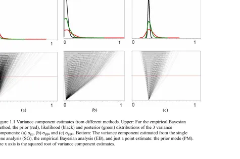
Figure 1.1 shows the variance component estimated from the single gene analysis and from the Empirical Bayes analysis. The global distributions of the 14010 variance component estimates from the single gene analysis (the red curves in the upper three graphs) are flatter and widely spread; while the posterior distributions (the green curves) are sharper and more concentrated. The bottom three graphs show how the single gene estimates shrink towards the prior distribution to produce the posterior estimates (only one point, the mode, of the prior distribution is shown). The posterior estimates can be viewed as an optimal compromise between the single gene estimates and the prior.

15

Figure 1.1 Variance component estimates from different methods. Upper: For the empirical Bayesian method, the prior (red), likelihood (black) and posterior (green) distributions of the 3 variance

components: (a) σgij, (b) σgijk and (c) σgijkl. Bottom: The variance component estimated from the single gene analysis (SG), the empirical Bayesian analysis (EB), and just a point estimate: the prior mode (PM). The x axis is the squared root of variance component estimates.

(a) (b) (c)

Number of significant genes

Bonferroni False Discovery Rate

Contrast

S.G.A.

E. B.

S.G.A.

E. B.

Male1_vs_CS 0 5 0 38

Male1_vs_OR-R 0 24 0 91

Male1_vs_Male2 0 9 0 28

Male1_vs_Virgin 0 7 0 48

CS_vs_OR-R 0 33 0 276

CS_vs_Male2 0 22 0 209

Cs_vs_Virgin 0 37 0 183

OR_R_vs_Male2 0 50 0 184

OR-R_vs_Virgin 0 48 0 190

Male2_vs_Virgin 0 9 0 68

Researchers are interested in all 10 possible pair-wise comparisons be-tween the 5 state levels. Table 1.1 gives the number of genes showing sig-nificant expression for each of the 10 contrasts. Multiple testing is adjusted by both Bonferroni (left columns) and false discovery rate (right columns). In both cases, the Empirical Bayes approach is able to declare hundreds of significant genes where the single gene analyses declare none.

1.4

Simulation Study

A Monte Carlo simulation study is performed to investigate (1) some statisti-cal properties of the empiristatisti-cal Bayes estimators of the variance components, as compared to the single gene analysis estimators, and (2) the type I error and power of the statistical test.

Simulation Design:

Data containing 5500 genes are generated. The experiment design struc-ture is exactly the same as that of the Drosophila data. For each gene, the response variable is:

1. The means of state 2, 3, 4 of gene g then take value 0.25 cg, 0.5 cg and 0.75 cg.

For example, to create data for geneg, the random effectsprep(state)gij,

chip(state×prep)gijk and γgijkl are generated independently from each of the three normal distributions with mean 0 and variances σ2_gij, σ2_gijk and σ2_gijkl, respectively. Those three variance components take values as the parameter estimates from the single gene analysis of the real dataset. For the fixed effects, the 20 probe measures take values as the parameter estimates from the real data as well. But the treatment means (stategi) have to be adjusted, since in the real dataset the treatment differences are too small and non-significant. Given the three variance components and the design structure, we first calculate the standard deviation of the contrast of two treatment means. The mean of state 1 is set to be 0 and the mean of state5 is set to be z folds of the standard deviation (for an initial setting, z = 2). After the initial dataset of 500 genes are generated, treatment mean difference between state 1 and state 5 is tested for each gene with the mixed model. The statistical power is estimated by the proportion of the number of the significant tests over all 500 tests. If this proportion is less than 0.9, then the treatment difference is set to be larger (i.e.,z is adjusted to take a larger value, e.g., z = 2.5) and the data are generated again. This process is repeated until the estimated power is greater than 0.9. Now the values of

stateg5 are set to be cg, and the means of state2,3,4 of gene g take value 0.25 cg, 0.5 cg and 0.75 cg.

A total of 50 Monte Carlo simulation replicates are generated. Analyses and results:

(1) Comparison of the two variance components estimators

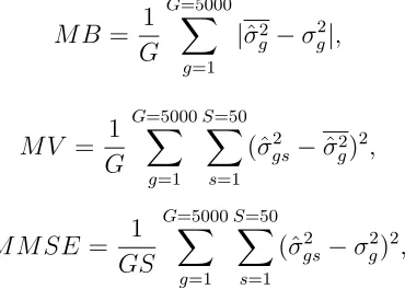
compo-nents estimators, the bias, the variance and the mean square error (MSE) of each estimator is estimated for every single gene. Since there are 5500 genes, we think it is appropriate to report the results at the global level. The better estimator should be the one having smaller mean bias (MB), mean variance (MV) and mean MSE (MMSE), where the mean is taken over all 5500 genes. Specifically, those statistics are defined as:

M B = 1

G

G=5000

g=1

|σˆ_g2−σ2g|, M V = 1

G

G=5000

g=1

S=50

s=1

(ˆσ_gs2 −σˆ_g2)2, M M SE= 1

GS

G=5000

g=1

S=50

s=1

(ˆσ_gs2 −σ_g2)2,

where ˆσ_gs2 is the variance component estimate for gene g, in sample s, ˆσ_g2 is the mean of ˆσ_gs2 in the 50 samples. The results are reported in Table 1.2.

The results show that, for all three variance components, the empirical Bayes estimators have smaller mean bias, smaller mean variance and hence smaller mean MSE than the single gene analysis (REML) estimators. At the first glimpse, the results seem unusual, since for any data set of given size, often bias and variance can not be controlled at the same time in estimation. An explanation will be given in the discussion section.

Figure 1.2 shows the comparison between the two estimators of the vari-ance component σ_gijkl2 (experiment error) over 5500 genes. It is obviously that the empirical Bayes estimates (blue) are more concentrated around the true values (the black horizontal line) than the REML estimates (red).

(2) The type I error and power

MMSE

(x10-4)

MB

(x10-3)

MV

(x10-4)

SGA EB SGA EB SGA EB

VC1 2.39 1.08 1.8 0.7 2.38 1.07

VC2 0.79 0.44 1.0 0.1 0.78 0.44

VC3 0.42 0.18 0.1 0.0 0.42 0.18

Table 1.2. Comparisons between the 2 variance components estimators

PVCS3

- 0. 4 - 0. 3 - 0. 2 - 0. 1 0. 0 0. 1 0. 2 0. 3 0. 4

gene

0 1000 2000 3000 4000 5000 6000

Figure 1.2. Comparison between the REML estimator (red) and the EB

estimator (blue) of the experiment error over 5500 genes. The x-axis contains

the gene numbers; the y-axis is the estimated experiment error, standardized

by the true value: (

g

g V

V

)/

. The length of the short vertical red or blue

lines on each gene represents the values of the estimates. The horizontal line

at 0 is the true parameter (self –standardized to be 0).

2

g

empirical Bayes algorithm, the test statistic is constructed by replacing the single gene analysis (REML) estimates of the variance components by the posterior empirical Bayes estimates. A natural question arises: what is the distribution of the new test statistic under the null hypothesis?

Unfortunately, the exact answer is unknown analytically. One possible solution is to numerically approximate the true distribution by applying cer-tain re-sampling techniques. However, the computation could be extremely intensive. In stead, we approximate the distribution of the test statistic by a standard normal distribution. This trick is usually applied when there is reasonable belief or evidence that the “true values” of the variance compo-nents are replaced in the test statistic. Since we expect (and observed in the simulation) the empirical Bayes estimates are much “closer” to the true values of the parameters than the single gene analysis estimates, this normal approximation is used in the algorithm.

It is thus important to know how good, especially from the test size point of view, this normal approximation is. For this purpose, we compare three approaches, the single gene analysis with t-test of 5 degree of freedom, the empirical Bayes analysis with normal test approximation and the single gene analysis with normal test given the true variance components, by investigat-ing the test size and the power. Based on the design of the simulation, there are 5000 non-significant genes and 500 significant genes, so the test size and power can be estimated at the same time. The results are reported in Table 1.3.

Test Size Power

Contrast SGA EB True SGA EB True

T1 vs. T2 (.25c) .049 .056 .050 .124 .146 .220

T1 vs. T3 (.50c) .050 .053 .053 .348 .480 .510

T1 vs. T4 (.75c) .047 .051 .050 .662 .810 .832

T1 vs. T5 (c) .048 .048 .043 .844 .904 .914

T2 vs. T3 (.25c) .050 .054 .053 .134 .166 .224

T2 vs. T4 (.50c) .051 .057 .057 .392 .518 .564

T2 vs. T5 (.75c) .049 .050 .044 .642 .724 .764

T3 vs. T4 (.25c) .048 .053 .049 .126 .184 .228

T3 vs. T5 (.50c) .051 .054 .045 .346 .412 .448

T4 vs. T5 (.25c) .046 .049 .049 .096 .146 .194

Table 1.3. Test size and power calculation

Densi t y

0. 0 0. 5

x

- 6 - 5 - 4 - 3 - 2 - 1 0 1 2 3 4 5 6

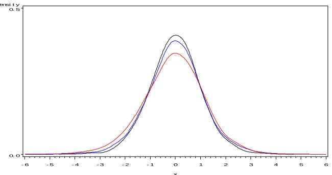
the test statistics under the null hypothesis (from the 5000 non-significant genes). It appears that, though the distribution of the empirical Bayesian test statistic (blue curve) is unknown, a standard normal distribution (black curve) may be a good approximation. On the other hand, the power of the empirical Bayes approach is noticeably higher than that of the single gene analysis with a t-test; but lower than that of the single gene analysis with a standard normal test given the true variance components. Combining results from both sides, we conclude that, comparing to the single gene analysis ap-proach, the empirical Bayes approach does improve the power of detecting true significant genes.

1.5

Discussion

Microarray data contain thousands of genes observed under the same ex-perimental design structure, sometimes involving several random factors, or variance components. We may treat the variance component estimates ob-tained from the single gene analysis as a realization from a prior distribution. In this way, the low power caused by small sample size may be improved by integrating information from all genes.

The posterior density is

sim-ulated from the independence chain algorithm; and (2) both pr(σ_AC2 and

p_g(σ2_AC) are inverted Gamma densities, so that the parameters in pg(σ2AC) can be easily estimated (as shown in data and methods). This is the reason that we estimate pg(σAC2 ) instead of fg(σAC2 ).

The empirical Bayes method can be thought as a statistical shrinkage method (actually, in general all Bayes estimators can be thought as shrink-age estimators). Like other shrinkshrink-age methods, such as the ridge regression (Hoerl and Kennard, 1970) and the Least Absolute Shrinkage and Selec-tion Operator (LASSO) (Tibshirani, 1996), this method trades off decreased variance for possibly increased bias in parameter estimation. During the shrinkage process, the variance of the variance component estimator is ex-pected to be reduced, while large posterior bias may be introduced if the destination of the shrinkage, in our example, the prior, is biased from the true values. However, in this empirical Bayes method, the prior density of each variance component is estimated from all 14010 genes. The histogram plot of the estimates over the 14010 genes gives a pretty good indication on the “true” distribution of the variance component. The simulation results show this estimated prior density represents the true distribution well enough so that the shrinkage (posterior) estimator not only has smaller variance as expected, but also has smaller bias than the REML estimator (the REML estimator is known to be asymptotically unbiased, but for small sample, i.e., in this Drosophila data set, it could be biased). Overall, for small samples, the empirical Bayes method tends to produce variance component estimators with smaller MSE than the REML estimators.

on other parameters (i.e., treatment means). This makes it possible that the hypothesis testing, including composite comparisons between treatments, is performed in a regular way (“regular” means in a classic linear mixed model framework) with the differences being that the posterior estimates of the vari-ance components are held constant in the final analysis and the test statistics is reasonably assumed to be approximately normally distributed. These fea-tures largely simplify the analysis and reduce the computational burden. This kind of analysis is readily performed using mixed model software such as SAS Proc Mixed.

The real data example in this paper is from Affymetrix oligonucleotide array data, and represents a case where treatment effects are somewhat sub-tle. The proposed approach borrows strength across all of the genes in a classical fashion and greatly increases the number of significant genes. The approach can be used in any case where a general mixed model is appro-priate, including those applied two-color cDNA array data (i.e., Jin et al, 2001).

1.6

Future Work

Chapter 2

Estimating and Testing Linkage

Disequilibrium Patterns by

Multiple Order Markov Chains

and the Linkage Disequilibrium

Map

2.1

Introduction

Many common diseases, such as cystic fibrosis, diabetes, cancer, stroke, schizophrenia, heart disease, asthma, etc, are usually caused by the com-bined effects of genetic variants and environmental factors. The efforts of defining and hunting for those factors have never ceased. However, until today, except for some diseases with single Mendelian genetic factors (e.g., cystic fibrosis), only very a few successes have been declared for the much more common complex diseases (e.g., all other diseases listed above).

of the underlying biological mechanism helps to increase the resolution of the mapping results. See Kerem et al, (1989) and Riordan et al, (1989) for ex-amples of the linkage mapping on cystic fibrosis; and see Weir (1996) for a brief review on some statistical issues related to linkage mapping. In complex disease studies, however, linkage mapping often produces weak and inconsis-tent results. In contrast to Mendelian diseases, a large number of genetic variants are likely involved in the complex diseases, with small contribution from each variant. Limited by sample/pedigree size, the resolution of the linkage mapping is relatively low, often in the range of 1 centiMorgans, or roughly 1 million bases in human. This is too wide for further molecular studies.

In a typical LD mapping study in a natural population, a random sample of uncorrelated individuals is drawn. For each individual in the sample, two types of data are collected, the phenotype data and the genotype data. The phenotype data, which may also be called “traits”, quantify the physical ap-pearance and characteristics of an individual. The data can be continuous, such as body weight or blood pressure (quantitative trait); or categorical, such as disease status (categorical trait). The genotype data contain infor-mation of the genetic constitution of an individual through genetic markers, the DNA sequence variations. The locations of the genetic markers and the specific allele at each marker of each individual are recorded. In recent years, the single nucleotide polymorphism (SNP) markers have been widely used in LD mapping. It is estimated that there could be as many as 10 million SNP markers in human populations (roughly 1 SNP every 300 bases), which constitute more than 90% of the total variation in human genome (HapMap website). These high-density SNP markers are desirable for a genome-wide scan for disease alleles. In this study, the proposed method is developed for SNP markers.

Each SNP marker usually has two alleles and hence is usually modeled as a Bernoulli random variable. The statistical correlation γ (a LD measure) between two loci has the same magnitude, but maybe opposite signs, no matter which two alleles are considered. Thus for SNP markers, the two-locus γ may be simply understood as a measure quantifying the correlation between these two Bernoullivariables (this may not be true if a marker has multiple alleles).

between the markers and the trait.

A commonly used strategy in LD mapping is to evaluate the association betweeneachsingle marker and the trait by some statistical test. The philos-ophy underlying the test is that the markers that are significantly associated with the trait may be close to the disease allele, or themselves may be the disease alleles (the so-called Quantitative Trait Nucleotide, or QTN). By ap-plying this single marker analysis, each marker is tested independently. The correlations among markers are not considered. The statistical power of this approach could be limited.

Several methods for multiple-marker LD mapping have been proposed (Terwilliger, 1995; Devlin, et al, 1996; Xiong, et al, 1997). In those meth-ods, multiple markers in a specific genome region are included in a likeli-hood model with all genetic parameters estimated simultaneously. Compared to the single marker analysis, the statistical power is enhanced. However, strictly speaking, these methods can be viewed as a simple “combination of multiple single marker analysis”(McPeek and Strahs, 1999). The informa-tion of the LD background is still not modeled and used in the analysis, as commented by Jorde (Jorde, 2000).

The two-locus LD is a key measure for the single marker analysis. How-ever, to fully characterize a p biallelic marker system, (2p −1) correlation measures are needed. This includes C_p1 single marker allelic frequencies; C_p2

2004). But unlike the well studied two-locus LD, very few LD mapping stud-ies and population genetics studstud-ies are based on multiple-locus LD measures (see Hastings, 1984 for an example).

One apparent obstacle is how to feasibly model the multiple-locus LD and to use this information in the LD mapping studies. The number of multiple-locus LD measures could be extremely large, even when p is moderate. In practice, not all LD can be estimated, since in general not all 2pdifferent types of gamete can be observed in a finite sample. Also, the sample distributions, or even the variance, of those LD estimators are difficult to obtain. So it is hard to test the significance of these LD measures, especially for higher order (e.g., when order>3) LD (Weir, 1996). Further, even if the LD background can be well modeled, it is not clear how these LD measures can be efficiently used in LD mapping to improve statistical power.

used only in one or several candidate gene regions with very a few markers (personal communication with Dr. D.Y.Lin).

Does this complicated haplotype approach have higher statistical power than a series of simple single marker analysis? There is no straight answer to this question. Some studies suggest that the results largely depend on the local LD patterns. It seems that the haplotype model performs better in a local chromosome region where markers are in higher order LD, but not as well if markers are in lower order LD (Akey, et al, 2001; Long and Langley, 1999; Kaplan and Morris, 2001; Zhang, K et al, 2002).

In summary, the single marker analysis ignores the correlation among markers. The approach is simple but it may not be sufficient. The haplotype approach takes all LD background into account, but it is not simple and its application is limited. Obviously, a logical improvement is to find a balance between the two extreme models based on the local LD patterns. Sharing similar idea, Zhang, X., et al (2003) developed the Bayesian Adaptive Re-gression Splines (BARS) method aiming to “bridge the gap between single locus and haplotype-based tests”. In this method, a statistic (e.g., LD) from single marker analysis is obtained first and then a single estimation of the dis-ease locus is made by adjusting all marker information with a nonparametric regression.

We will take a different approach, which is more straightforward. Stim-ulated by the genetic map in linkage analysis, an LD map is constructed as the first step to summarize the local multiple-locus LD patterns. Then a likelihood based mapping method will be developed based on this local LD map. This chapter will mainly focus on the first step. The second step will be briefly discussed in the section of future studies.

At the first step, the statistical challenges are:

local multiple-locus LD patterns among, possibly, millions of SNP markers and;

(2) to construct an LD map, where the information of local LD pattern is represented in a way such that this information can be used in LD mapping. For challenge (1), a direct approach is to estimate and test all the multiple-locus LD. However, as discussed previously, there are many technical difficul-ties. In this chapter, we introduce a simple approach involving the multiple-order Markov chain models. This approach summarizes the local higher multiple-order LD patterns along the chromosome in terms of the order of Markov chains. The relations between the Markov chain parameters and the LD measures are explored. A better fit of a Markov chain model of a certain order in the local chromosome region indicates the existence of the same and lower order of LD patterns in this region. Consequently, a local LD map can be constructed based on the multiple-order Markov chain model fitting results. The idea of LD map comes from the concept of the linkage map in de-signed cross populations or pedigrees. It is known that a specific type of correlation pattern among multiple markers can be well modeled by some ge-netic maps in a linkage analysis in experimental cross populations. Through a designed cross from inbred lines, the recombination events can be observed. A linkage map can thus be generated by modeling the interference effects of double recombination with different assumptions. The Haldane genetic map assumes the interference effects are absent, i.e., the recombination event in one interval is independent of those in any other intervals. Between two loci 1 and 2, the map distance x₁₂ is defined as a logarithm function of the recombination rate c₁₂. Specifically,

x₁₂=−0.5 log(1−2c₁₂).

and 2, per gamete, per generation. Depending on the specific cross design, the quantity (1−2c₁₂) (the “linkage parameter”) is related to the statistical correlation γ. For example, in the backcross design, γ₁₂ = (1−2c₁₂). In this case x₁₂ = −0.5log(γ₁₂). Further, assuming no interference, for loci 1, 2, 3 in this order, (1−2c₁₃) = (1−2c₁₂)(1−2c₂₃), or γ₁₃ = γ₁₂γ₂₃. This is a specific type of correlation pattern (multiplicative correlation) among multiple markers, which directly implies x₁₃=x₁₂+x₂₃.

Note that, just from a statistical point of view, if three binary random variables M₁, M₂, M₃, are truly generated from a Markov chain model of order 1 (M C1), then it can be easily shown that:

γ₁₃=γ₁₂γ₂₃. (Eq.1) SoEq.1 is anM C1 property. Consequently, if all SNP markers in a chromo-some region can be appropriately modeled by M C1, then an additive map can be constructed with map distance being the logarithm of the statisti-cal correlation γ. The Haldane genetic map is such an additive map with a Markov chain interpretation, since its assumption of no interference satisfies the Markovian property.

When an LD map is to be constructed from a set of SNP data, certainly, it is inappropriate to simply assume that the markers are well modeled by

2.2

Methods and Results

2.2.1

Model settings and vocabularies

The method has been developed under some simplified situations. Consider a dataset containingC independent haplotypes from a natural population with random mating. Hardy-Weinberger equilibrium is assumed. The hyplotype data can be obtained either directly from biological experiments (e.g., Deluca et al, 2003) or estimated from diplotype data by some statistical methods (Weir and Cockerham, 1979; Hawley and Kidd, 1995; Long, et al, 1995).

Suppose chromosomechasmc biallelic SNP markers, with the two alleles (states) denoted as 1 and 0. The SNP marker i is modeled by a Bernoulli

random variable Mi for i = 1, ..., mc, which has observation mi,c(mi,c = 1,0) on chromosome c (c = 1, ..., C). Let Pi = P(Mi = 1) be the prob-ability of allele 1 for marker Mi in the population. H(i,k) is the

haplo-type containing k consecutive markers starting from the ith marker, e.g.,

Mi, Mi+1, ..., Mi+k−1. hc(i,k), a k × 1 vector of the observed H(i,k) on the

chromosome c, i.e., hc(i,k) = [mi,c, mi+1,c, ..., mi+k−1,c]. P(H(i,k) = hc(i,k)) is

the population frequency for the specific haplotype hc(i,k). The conditional

probability that a marker Mi takes value mi,c given its previous r markers

Mi−r, ..., Mi−1 taking values hc(i−r,r), is denoted as P(Mi = mi,c|H(i−r,r) =

hc(i−r,r)), or P((mi,H_(i,c(i₎−,hr,r_c()_i)_−r,r)). If we assume the haplotype counts follow a

multinomial distribution (Weir, 1996), the maximum likelihood estimate of the haplotype frequency P(H₍i,k)) is: ˆP(H(i,k)) = ( counts of H(i,k))/n; the

conditional probability P(Mi = mi,c|H(i−r,r) = hc(i−r,r)) can be estimated

as ˆP(H_{(i−r,r+mi,c)})/Pˆ(H_(i−r,r)), where H_{(i−r,r+mi,c)} represents the haplotype [Mi−r, ..., Mi−1, Mi =mi,c].

The two-locus LD measure D₁₂ between locus 1 and 2 is defined as:

where P₁₂ = P(H₍₁,2)). For three loci, the definition of three-locus LD by

Bennett (1954) is adopted:

D₁₂₃ =P₁₂₃−P₁D₂₃−P₂D₁₃−P₃D₁₂−P₁P₂P₃,

where P₁₂₃ =P(H₍₁,3)).

D is a normalized version of D, which is defined as:

D₁₂=

D₁₂/max(−P₁P₂,−(1−P₁)(1−P₂)) if D₁₂<0, D₁₂/min(P₁(1−P₂),(1−P₁)P₂) if D₁₂>0.

Another two-locus LD measure γ₁₂ is defined as:

γ₁₂ =D₁₂/P₁(1−P₁)P₂(1−P₂).

It can be shown that, D₁₂, γ₁₂ are the statistical covariance and correlation between the two Bernoulli variables M₁ and M₂, respectively.

A third two-locus LD measureρ is defined as (Zhang, W. et al, 2002(a)):

ρ₁₂=|D₁₂|/min[P₁P₂, P₁(1−P₂),(1−P₁)P₂,(1−P₁)(1−P₂)].

In random samples, ρ is numerically equal to D. An LD map constructed based on this measure will be briefly mentioned in the Discussion section.

2.2.2

Moving Multi-order Markov chain

Multiple-order Markov chain models have been used to measure how far the correlations between adjacent DNA bases extend along a chromosome (Weir, 1996). In this study, a multiple-order Markov chain model is applied to measure the complexity of the higher order LD patterns.

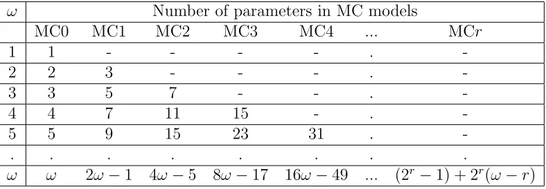
Table 2.1: The Number of Parameters in Multiple-Order Markov Chain Mod-els for windows of length ω

ω Number of parameters in MC models

MC0 MC1 MC2 MC3 MC4 ... MCr

1 1 - - - - .

-2 2 3 - - - .

-3 3 5 7 - - .

-4 4 7 11 15 - .

-5 5 9 15 23 31 .

-. . . .

ω ω 2ω−1 4ω−5 8ω−17 16ω−49 ... (2r−1) + 2r(ω−r)

interest, then the whole region can be viewed as a window with the maximum size mc; if more detailed local information is of interest, the window size should be set small. For a window with specific sizeω (ω ≤mc), the highest order of Markov chain that can be applied is (ω−1); while the lowest order is always 0, implying independence among markers. For simplicity, the Markov chain of order r is denoted as M Cr.

The Markov chain models applied in this study are non-stationary. All transition probabilities are locus-specific. For a chromosome region contain-ing ω markers (M₁, M₂, ..., Mω), theM Crmodel has (2r−1) initial parame-ters and (2r(ω−r)) conditional parameters. The numbers of parameters are summarized in Table 2.1.

The likelihood of observing hc(1,ω) = (m1,c, m2,c, ...mω,c) is a function of the Markov chain order r:

Lc(M Cr) = P(H(1,r−1) =hc(1,r−1))×P(Mr|H(1,r−1) =hc(1,r−1))×

For C independent chromosomes, the total likelihood is

L(M Cr) = N

c=1

Lc(M Cr).

There are two types of parameters in the likelihood, the 2r −1 initial parameters P(H₍₁,r−1) = hc(1,r−1)) and the 2r(ω −r) conditional

probabili-ties P(Mr|H₍₁,r−1) =hc(1,r−1)), ... , P(Mω|H(ω−r+1,r−1) = hc(ω−r+1,r−1)). As

shown in last section, the maximum likelihood estimates of both types of parameters can be obtained by assuming that the haplotype counts follow a multinomial distribution. In the sample, the likelihoodL(M Cr) is calculated by replacing all parameters with their maximum likelihood estimates. Note that only the observed haplotypes contribute to the likelihood.

Within each moving window of size ω, Markov chain models with dif-ferent orders, from 0 to r, are applied to fit the data and compared by the Bayesian information criterion (BIC). Some studies suggest that the BIC is a valid criterion of estimating the orders of Markov chain models (Katz, 1981; Cisizar and Shields, 1999; Finesso, 1992). The BIC is defined as:

BIC(r) =Constant−2log(L(M Cr)) +dr log(sr),

where dr = (2r −1) + 2r(ω − r) is the number of free parameters in the

M Cr model; sr is the number of observations, i.e., n(ω−r), the number of subsequences of length (r+ 1). The order of the M C model with the smallest BIC value is selected and recorded as a statistic associated with this window. As the window moves along the chromosome, a series of such statistics are collected. Those statistics provide a summary of the Markov chain model fitting results in each window along the chromosome.

0 1

2 3

4

Marker Location

Order of Markov Chain

236

249

269

323

358

385

420

440

484

543

551

639

644

731

1042

1524

1685

2127

2738

3554

4694

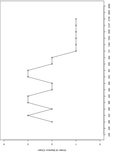
Raleigh population. As in many other statistical methods, the markers with minor allele frequency less than 0.05 (15 markers) are not used in the analy-sis. The locations of the remaining 21 markers are shown in Figure 2.1. Among the 21 markers, 14 are in the promoter region (236-731bp) and 7 are in the remainder of the gene region (1042-4694bp). Markov chain models with order from 0 to 4 are applied to fit the data. Since the detailed local LD information is desired in this study, the window size is set to be 5 (the smallest possible for the M C4 model). So, in this example, m=21, ω=5,

r=4. In Figure 2.1, the first point at the (269, 2) indicates that, in the first window containing 5 markers at location (236, 249, 269, 323, 358), centered at location 269, the BIC criterion chooses theM C2 model as the best model for this window. As the window moves 1 marker right along the chromo-some, to (249, 269, 323, 358, 385), the M C3 model fits data best and gives the point (323, 3). And so on ..., until the window reaches the last 5 markers (1685, 2127, 2738, 3554, 4694), where the M C1 model fits data best.

Summarizing the LD patterns (see next section for relations between the Markov chain orders and the higher order LD) in this way provides more local information than the popular two dimensional pairwise LD plot (Figure 3.a., DeLuca et al, 2003). In the pairwise LD plot, many significant two-locus LD are detected, but their locations seem to be randomly distributed in the two dimensional plot. In Figure 2.1, it is obvious that the LD patterns change dramatically from the promoter region (before locus 731) to the remainder gene region (after locus 731). This result may suggest that, in the Ddcgene, fewer recombination events have occurred in the promoter region than in the coding region (see the example 1 in Application).

to be 4. Theoretically there is no such restriction (we may set ω =m= 21, and fit MC20 model to the data). But in real data analysis, limited by the number of observed haplotypes in a finite sample, a large number of parameters will either be 0, or not be estimable if the order of Markov chain model is too high. To our experience, we have not observed any examples in whichM C5 model or higher (i.e., six-locus LD) is selected by BIC, either in real data or simulated data. So in practice, we suggest to restrict the maximum order of Markov chain to be 4 to avoid the non-estimable problems and to save computing time.

2.2.3

Explanation of the results of the multi-order

Markov chain modeling in terms of LD measures

The interpretation of the results of the Markov chain modeling is not trivial. For example, if the result shows that the M C2 model is a better model than the M C1 model in a certain window, what do we learn from it? Since the

M C2 model characterizes the dependence among three markers, intuitively the result may suggest that in average the LD extends to three markers in this window. But the explicit patterns on how the three markers are correlated are still not clear.

In order to clarify the specific correlation patters embodied in each order of M C model, the connection between the parameters of the M C models and the multiple-locus LD measures need to be established. Since both are functions of hyplotype frequencies, the connection can be built by re-parameterizations.

When two M C models of different orders are compared, the higher order

full model parameters. For example, consider the simplest case where the

M C0 model and the M C1 models are compared within a window of size 2 containing markersM₁, M₂. Since theM C1 model has 3 parameters and the

M C0 model has 2, only one constraint is expected. For M C models, how the lower order M C model is nested in the higher order M C model is not clear, since the parameters in each order ofM C model are different. In order to determine this constraint, the 3 parameters, P₁,P₂ and γ₁₂ are expressed in terms of the 2 M C0 model parameters P₁ and P₂. It is obvious that, the constraint is γ₁₂ = 0. This is the interpretation of comparing the M C0 model with theM C1 model in this two-marker-window.

Now consider a more complicated example. In a window of size 3 with markers M₁, M₂ and M₃, what are we examining when we compare the reducedM C1 model with the full M C2 model?

For a M C1 model, there are 5 parameters (P₁, P(M₂ = 1|M₁ = 1) =

P₍₁(2_,,₁₎1), P(M₂ = 0|M₁ = 0) = P₍₀(2_,,₀₎1), P(M₃ = 1|M₂ = 1) = P₍₁(3_,,₁₎2) and

P(M₃ = 0|M₂ = 0) =P₍₀(3_,,₀₎2). To fully model 3-biallelic markers, 7 parameters are necessary: the 3 parameters of single marker alleles, P₁, P₂, P₃; the 3 pair-wise LD parameters, D₁₂, D₂₃ and D₁₃; and the 1 parameter of 3-locus LD,D₁₂₃. Note that instead ofγ, D is used here since the reparameterization in D is easier.

The 7 parameters can be expressed with the 5 M C1 model parameters:

P₁ =P₁;

P₂ =P₁P₍₁(2_,,₁₎1)+ (1−P₁)(1−P₍₀(2_,,₀₎1));

P₃ =P₂P₍₁(3_,,₁₎2)+ [P₁(1−P₍₁(2_,,₁₎1)) + (1−P₁)P₍₀(2_,,₀₎1)](1−P₍₀(2_,,₀₎1));

D₁₂=P₁(P₍₁(2_,,₁₎1)−P₂);

D₁₃=P₁[P₍₁(2_,,₁₎1))P₍₁(3_,,₁₎2)+ (1−P₍₀(2_,,₀₎1))(1−P₍₀(3_,,₀₎2))]−P₁P₃;

D₁₂₃ =P₁P₍₁(2_,,₁₎1)P₍₁(3_,,₁₎2)−P₁D₂₃−P₂D₁₃−P₃D₁₂−P₁P₂P₃.

Two constraints on those 7 parameters are expected. Recall that the

Eq.1 is a property of M C1 model, so γ₁₃ = γ₁₂γ₂₃, or equivalently D₁₃ =

D₁₂D₂₃/P₂(1−P₂) should be one constraint. Intuitively, another constraint should be a function containing the three-locus LD, since the M C2 model does contain parameters involving all 3 markers while theM C1 model does not. Some derivations determine the second constraint: (C2) D₁₂₃ = (1− 2P₂)D₁₃. Both constraints can be easily verified given the reparameterization formula above.

So, (C1) and (C2) are the two constraints in terms of the LD measures for the comparison of the reduced M C1 model versus the full M C2 model in this 3-marker window.

Some important comments:

(I) The way we search for constraints seems to be somewhat unusual in statistics. Often, for a series of nested models, the difference in the parame-terizations between the reduced model and the full model is obvious, which indicates the contents and the interpretations of the comparison. For the multi-order Markov chain models, however, the nested structure is ambigu-ous. So, to explain the comparison results, the Markov chain parameters are re-parameterized by the LD measures. Thus the comparison between M C

models can be interpreted by the constraints on the LD measures. In the

(II) One definition of D₁₂₃ is (Bennett, 1954):

D₁₂₃ =P₁₂₃−P₁D₂₃−P₂D₁₃−P₃D₁₂−P₁P₂P₃.

It is basically the statistical covariance of the 3 markersM₁, M₂,M₃ (Wang, 2001). For the 3 markers, if theM C1 model is preferred over theM C2 model, it makes intuitive sense that the three-locus LD is absent. However, we observe thatD₁₂₃ = (1−2P₂)D₁₃ = 0. If we let: D∗₁₂₃=D₁₂₃−(1−2P₂)D₁₃, then the constraint C2 is simplified as: D₁₂₃∗ = 0. The quantity D∗₁₂₃ can be thought as a slightly modified version ofD₁₂₃, i.e.,D₁₂₃∗ =P₁₂₃−P₁D₂₃−(1−

P₂)D₁₃−P₃D₁₂−P₁P₂P₃. One interesting observation is that,D∗₁₂₃is sensitive to the marker order but D₁₂₃ is not, i.e., D₁₂₃ = D₁₃₂ = D₂₁₃, but generally

D∗₁₂₃ = D∗₁₃₂ = D∗₂₁₃. Note that this is not a problem for two-locus LD. However, since in almost all datasets, the order of the markers is known,D₁₂₃∗

may have advantage by utilizing more information than D₁₂₃. Nevertheless, expressed in D₁₂₃∗ , the constraint C2 is now a simple null hypothesis, which allows us to further test it by a likelihood test (explained later).

(III) The window size ωalso determines the constraints. The window size effect has been briefly discussed in the last section. Now let us take a deeper look. All results derived above assume a small window, i.e., to compare