Exploring noncoding variation in human diseases and disorders through targeted sequencing and functional prediction

(1)

Exploring non-coding variation in human diseases and disorders

through targeted sequencing and functional prediction.

Lilian Elizabeth Hunt

University College London

and

The Francis Crick Institute

PhD Supervisor

:

Dr Greg Elgar

A thesis submitted for the degree of

Doctor of Philosophy

University College London

October 2017

(2)

Declaration

I, Lilian Hunt, confirm that the work presented in this thesis is my own. Where information has been derived from other sources, I confirm that this has been indicated in the thesis.

(3)

Abstract

The identification of non-coding single nucleotide polymorphisms (SNPs) and short insertions or deletions (indels) that are causative or contributory to human diseases and disorders is limited by the functional knowledge of the non-coding genome. This work demonstrates multiple approaches to elucidate functional variation in the non-coding genome by using homogenous populations or pedigrees of individuals with shared diseases and disorders, including Obesity, Schizophrenia, Anosmia and Mitochondrial Depletion Syndrome. A vast bank of non-coding variation has been created and can be utilised for population analysis. Using supporting evidence of developmental contributions to the disorders studied and genome interaction data, high coverage sequencing of targeted regions and subsequent bioinformatics analysis suggests multiple new disease-associated non-coding variants. Combining available variant function predictor tools and publicly available

functional data, a selection of variants are prioritised as potentially causative or contributory and their affect on the region’s function in development as an enhancer is assessed in

Zebrafish. In addition, deep-sequencing and bioinformatics analysis in mouse models of MPV17 deletion contributes to the understanding of mitochondrial depletion syndrome.

(4)

Impact Statement

This work provides a significant contribution to the field of human genomics, specifically non-exonic sequencing and the variation that lies therein. The importance of exploring and understanding variation in non-exonic regions is paramount to understanding human diseases and disorders, specifically those resulting from embryonic development. Utilising genomic sequencing, as presented here, not only increases our understanding of general population variation, but also allows us to look for pathogenic mutations. The methodology of targeted sequencing and the variant calling and analysis pipelines could be applied in future in other instances of human developmental disease with a hypothesised non-coding variant cause. This top-down approach could also provide further insight to decoding the non-coding genome by continuing the work presented here, collating other functional non-coding mutations, and exploring the immediate sequence surrounding them. By using conserved non-coding elements as a base for much of this work, the functional prediction of the regions sequenced is already biased in a positive way. With further understanding of other regulatory element markers, other predicted enhancer regions could be sequenced in a similar manner.

All chapters in this work contribute to the understanding of a variety of human diseases: Isolated Congenital Anosmia, Schizophrenia, Obesity and Mitochondrial Depletion Syndrome. Understanding the underlying genetic contributions to human diseases and disorders can spark lines of investigation into treatments (such as pharmacological

interventions) and preventions (including genetic counselling of prospective parents). With such a vast understanding of coding mutations and their contribution to diseases, this work looks to shift the future focus onto the other 98% of the human genome, a vast expanse of information that is yet to be fully decoded.

(5)

Acknowledgement

I’d like to acknowledge my supervisor Greg Elgar, for both supporting me and giving me the freedom to carry out this work. I’ve had a whale of a time. I’d also like to acknowledge Jim Smith, not only as a member of my thesis committee but as a mentor and ally. I’d like to thank Michael Simpson and Pete Scambler for their invaluable contributions as part of my thesis committee. I’d also like to acknowledge and thank Boris Noyvert and his irreplaceable bioinformatics help, as well as all the members of the Elgar lab, past and present, who I have worked with during this PhD: Joe Grice, Johanna Fischer, Stefaan Pauls, Laura Doglio, Htoo Wai, Maria Greco, Bathilde Ambroise and Chloe Moss. I’d also like to thank all of the Gilchrist lab, with whom we have shared space, time, drinks and many excellent ideas. All of this work and my survival as a student in London would not have been possible without the funding of the Medical Research Council and the support of The Francis Crick Institute and former National Institute for Medical Research.

I could not have done any of this, especially finish this thesis, without the incredible support of my fiancée Holly. Thank you.

On a personal note, there are many others who I owe this work and my PhD experience to: Rachel, Simon, Naomi, Jed, Derek, Rita, Theresa, Pete, Sissy, Sam, Alex, Rick and Morty.

(6)

4.2.4.1 Comparative population genetics is restricted by publicly available data, including poor coverage of the non-coding genome and few ethnically comparable samples 107 4.2.4.2 Use of the variant-prioritisation pipeline (developed in ‎4.2.2) identifies Schizophrenia associating variants with predicted functional consequences ... 110

4.2.4.3 Functional predictions of disease associating SNPs prioritising variants for functional analysis ... 111

4.2.4.4 Enhancer assay in zebrafish confirms neural developmental activity of CNE surrounding an associating variant upstream of POU3F3 ... 112

4.2.4.5 Predicted consequences of variant allele chr2:104496685 T>G ... 115

4.3 Discussion and Conclusions ... 118

Chapter 5. Targeted sequencing of mitochondrial DNA in MPV17-/- mice discovers no effect of dNTP insufficiency on mutational load and mtDNA replication fidelity... 124

(9)

5.1 Background ... 124

5.2 Results ... 126

5.2.1 dNTP insufficiency does not alter the mutational load in Mpv17-/- liver mtDNA 126 5.2.2 MPV17 deficiency does not alter the mutant load of brain mtDNA. ... 129

5.3 Discussion and conclusions ... 132

Chapter 6. Conclusions ... 134 Chapter 7. Appendix ... 137 7.1 Appendix Table 1 ... 137 7.2 Appendix Table 2 ... 146 7.3 Appendix Table 3 ... 148 7.4 Appendix Table 4 ... 150

7.5 Intellectual Disability and Epilepsy comorbidity sample and phenotype information ... 154

7.6 Isolated Congenital Anosmia patient phenotypes and pedigrees ... 162

7.7 Appendix Script 1 ... 164

(10)

Table of figures

Figure 1. Timeline of key advances in sequencing platform technology. ... 21

Figure 2. NGS sequencing as performed on Illumina platforms. ... 23

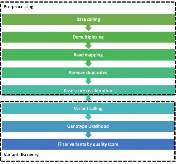
Figure 3. NGS data processing pipeline from sequence data to SNP and short InDel calling (Van der Auwera et al., 2013). ... 24

Figure 4. Regulation of gene expression by transcription factors ... 29

Figure 5. An example of JASPAR database information for FOXD1 TFBS (Mathelier et al., 2016). ... 31

Figure 6. Chromosome conformation capture (3C) technique overview. ... 33

Figure 7. Transient GFP enhancer assay in Zebrafish ... 50

Figure 8. The number of samples where 90% of bases have the coverage of each bin value. ... 57

Figure 9. Variant frequencies across the 2 Mb interval. ... 58

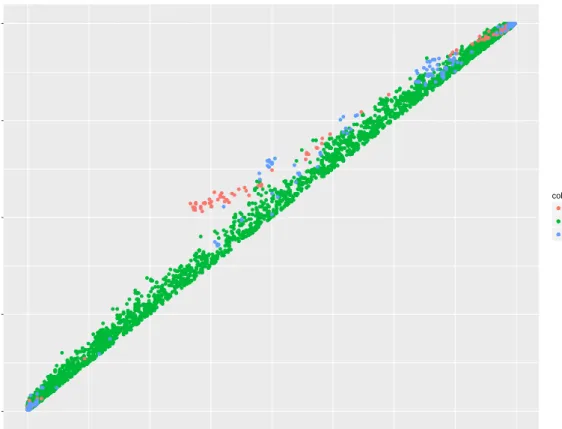
Figure 10. Global variant frequencies compared to cohort variant frequencies. ... 59

Figure 11 Cumulative frequency distribution of variants. ... 60

Figure 12. Full LD mountain plot of chr16:53500000-555500000 sequenced and exported from Haploview. ... 61

Figure 13. Minor allele frequencies for each variant across the 2 Mb interval compared between controls and cases. ... 62

Figure 14. AH44 LD block region exported from Haploview... 63

Figure 15. Novel association peak region exported from haploview ... 64

Figure 16. Association of individual SNPs to cases v controls. ... 66

Figure 17. Allele frequencies by age in Female GOYA cohort. ... 68

Figure 18 Age dependence of SNP rs12598453:C>G association to obesity. ... 69

Figure 19. Comparison of the SNP association data with previously published Hi-C data. 72 Figure 20. UCSC browser figure of the second association peak region (54820000-54860000) ... 74

Figure 21 WashU epigenome browser figure. ... 75

Figure 22. Development of the lip and palate in humans ... 84

Figure 23. CNE variant frequencies currently listed in 1000 Genomes database (phase 3). 90 Figure 24. Spread of average coverage of samples in each sequenced cohort. ... 91

(11)

Figure 25. Common variation between CLP samples shows sample mislabelling and

contamination ... 93

Figure 26. Identification of trios and confirmation of genders of samples using only variants called. ... 94

Figure 27. Visualisation of targeted sequencing and variant prioritisation pipeline. ... 96

Figure 28. Comparison of spread of scores for CNE variants in dbSNP141 by CADD and RegulomeDB... 97

Figure 29. Comparison of the spread of CADD scores within RegulomeDB scoring categories shows no significant trend in agreement between the two sets of data ... 98

Figure 30. Comparison of IDE cohort allele frequencies and 1000 Genomes global allele frequencies identifies multiple novel variants. ... 100

Figure 31. Comparison of CLP cohort allele frequencies and 1000 Genomes global allele frequencies identifies multiple novel variants. ... 101

Figure 32. CADD and RegulomeDB scores for variants following inheritance patterns of Anosmia in four European families. ... 103

Figure 33. CADD normalised scores plotted against the RegulomeDB scores for the same variant in European Anosmia affected families ... 103

Figure 34. hs422 VISTA Enhancer element expression in e11.5 mouse embryo ... 106

Figure 35. PCA showing overlap of Pakistani Schizophrenic cohort with SAS 1KG population. ... 108

Figure 36. HiC interactions in H1-ESC cells ... 113

Figure 37. 48hpf zebrafish embryo with showing neuronal GFP expression after 1-cell stage microinjection of B-Tol2:GFP. ... 114

Figure 38. Enhancer signal variations between zebrafish injected with the same construct (B). ... 114

Figure 39. CRCNE00007883 sequence level conservation shows chr2:104496685 is a non-variable base amongst vertebrate organisms. ... 115

Figure 40. Mouse mtDNA samples sequence coverage. ... 127

Figure 41. Proportion of misincorporated bases shown as proportions per base. ... 129

Figure 42. Proportion of misincorporated bases broken down by base. ... 130

Figure 43. The rate of misincorporation of bases across each position of the mitochondrial genome in mouse brain samples. ... 131

(12)

List of tables

Table 1. RegulomeDB scoring categories for SNPs ... 38

Table 2. PCR Primers used ... 48

Table 3. Study group details ... 56

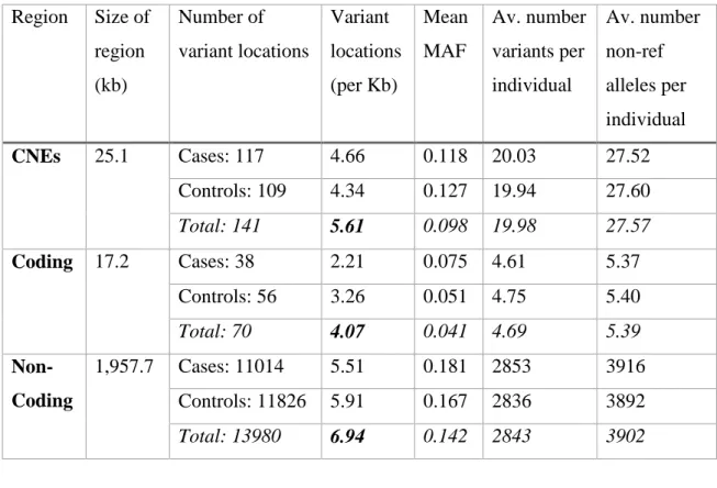
Table 4. Variant summary data for chr16q12.2 classified by functional region and BMI status ... 60

Table 5. Replication data using SNP rs12598453:C>G as a representative of the three SNPs referred to in the text ... 70

Table 6. Cohorts used in this chapter for CNE sequencing ... 82

Table 7. CNE targeted sequencing coverage of all cohorts ... 91

Table 8. SNPs in CNEs exclusive to CLP children, rare in 1000 Genomes European cohort. SNP 5:91019059 is a de novo heterozygous variant. All others are only found as homozygous in affected children. ... 99

Table 9. Novel variants discovered in cohorts undergoing targeted CNE sequencing . 101 Table 10. Family-specific pedigree tracing, using other affected and unaffected individuals as control populations... 102

Table 11. Prioritised familial variants in European families presenting Anosmia to be taken forward to functional studies ... 104

Table 12. Variant alleles associating with Schizophrenia ... 110

Table 13. CADD scores for Schizophrenia associating variants ... 111

Table 14. RegulomeDB scores of Scizophrenia associating variants. ... 112

Table 15. JASPAR output for WT sequence chr2:104496679-104496691 ... 116

Table 16. JASPAR output for variant sequence chr2:104496679-104496691 ... 117

Table 17. Mutational load in purified liver mitochondrial DNA of Mpv17-/- mice and controls. ... 128

Table 18. Mutational load in purified brain mitochondrial DNA of Mpv17-/- mice and controls. ... 130

Table 19. Obesity cohort information ... 137

Table 20. Obesity haplotypes ... 146

Table 21. Cleft lip/palate cohort sample and sex information ... 148

(13)

Table 23. IDE cohort clinical notes ... 154 Table 24. Anosmia sample information ... 163

(14)

Abbreviations

1KG 1,000 Genomes Project

3C Chromosome Conformation Capture 3C Chromosome Conformation Capture

4C Circularised Chromosome Conformation Capture

4C-seq Circularised Chromosome Conformation Capture-Sequencing A, C, G, T Adenine, Cytosine, Guanine, Thymine

AF Allele Frequency AMP Ampicillin ANOS Anosmia cohort ANOVA Analysis of Variance

BEB Bengali from Bangladesh

BLAST Basic Local Alignment Search Tool BLAT Basic Local Alignment Tool

BMI Body Mass Index

BWA Burrows-Wheeler Aligner software

CADD Combined Annotation Dependent Depletion Cas9 CRISPR associated protein 9

CASAVA De-multiplexing software made available by Illumina CEBPA CCAAT/Enhancer Binding Protein Alpha

CEU Utah Residents (CEPH) with Northern and Western European Ancestry ChIA-PET Chromatin Interaction Analysis with Paired-End Tag

ChIP-Seq Chromatin ImmunoPrecipitation-Sequencing CL±P Cleft lip with or without cleft palate

CLP Cleft Lip and Palate cohort CNE Conserved Non-coding Element

CNG Centre National de Genotypage, Evry, France CNV Copy Number Variation

CONDOR Conserved Non-coDing Orthologous Regions database CTCF CCCTC-binding factor

d.f degrees of freedom

dATP Deoxyadenosine triphosphate dCTP Deoxycytidine triphosphate

(15)

dGTP Deoxyguanosine triphosphate DHS Dnase 1 Hypersensitive Site DNA Deoxyribonucleic acid DNase DeoxyriboNuclease

dNTP Deoxyribonucleoside triphosphate dTTP Deoxythymidine triphosphate

E.coli Escherichia coli

EAF European Allele Frequency ENA European Nucleotide Archive ENCODE ENCyclopaedia Of DNA Elements

eQTL Expression quantitative trait loci

FAIRE Formaldehyde-Assisted Isolation of Regulatory Elements

FASTQ Text-based file format comprised of FASTA sequence and quality score encoded with an ASCII character

FGF Fibroblast Growth Factor

FGFR Fibroblast Growth Factor Receptor FIN Finnish in Finland

FOXD1 Forkhead Box D1 gene FOXO4 Forkhead Box O4

FTO Fat mass and obesity-associated protein also known as alpha-ketoglutarate-dependent dioxygenase FTO

FWER Family-Wise Error Rate GAF Global Allele Frequency GATK Genome Analysis ToolKit

GBR British in England and Scotland GERP Genomic Evolutionary Rate Profiling

GFP Green Fluorescent Protein

GIANT The Genetic Investigation of ANthropometric Traits consortium GIH Guajarati Indian from Texas subpopulation of 1000 Genomes

GIS Genome Institute of Singapore GO Gene Ontology

GOYA Genome-Wide Population-Based Association Study of Extremely Overweight Young Adults

(16)

GWAS Genome Wide Association Studies H1-ESC H1 human embryonic stem cell HapMap Haplotype Map

hESC Human Embryonic Stem Cells

Hi-C Hi-throughput chromosome confirmation capture sequencing HMR Human-Mouse-Rat alignment

HOXD9 Homeobox D9

hpf Hours post fertilisation HWE Hardy-Weinberg Equilibrium

ICA Isolated Congenital Anosmia ICH Isolated Congenital Hyposmia

IDE Intellectual Disability and Epilepsy cohort InDel Short Insertion or Deletion variant

IRX1 Iroquois Homeobox 1 IRX2 Iroquois Homeobox 2 IRX3 Iroquois Homeobox 3 IRX4 Iroquois Homeobox 4 IRX5 Iroquois Homeobox 5 IRX6 Iroquois Homeobox 6 IRXA Iroquois A gene cluster IRXB Iroquois B gene cluster

ITU Indian Telugu from the UK kb Kilobase

KO Knockout

LD Linkage Disequilibrium MAF Minor Allele Frequency

MAQ Mapping and Assembly with Quality software MDS Mitochondrial Depletion Syndrome

ML Mutation Load

MPV17 Mitochondrial Inner Membrane Protein Gene MPV17 mRNA Messenger RNA

mtDNA Mitochondrial DNA MZ MonoZygotic

(17)

NCBI National Centre for Biotechnology Information NGS Next Generation Sequencing

NHGRI National Human Genome Research Institute NOG Noggin

NR2F1 Nuclear Receptor Subfamily 2 Group F Member 1 OMIM Online Mendelian Inheritance in Man

PAKI Pakistani Populations

PANSS Positive And Negative Syndrome Scale PCA Principal Component Analysis

PCR Polymerase Chain Reaction PHRED PHRED-scaled scores

PJL Punjabi from Lahore, Pakistan POU3F2 POU Class 3 Homeobox 2

PTU 1-phenyl 2-thiourea RMAP Read Mapping software

RNA Ribonucleic acid RNAPII RNA Polymerase II

rNMP Ribonucleoside Monophosphates

RPGRIP1L RPGR-Interacting Protein 1-Like Protein SAS South Asian

SCHZ Schizophrenia cohort

SCN5A Sodium voltage-gated ChaNnel type 5 Alpha subunit SEM Standard Error from the Mean

SIFT tool to Sort Intolerant From Tolerant amino acid substitutions SNP Single Nucleotide Polymorphism

SNV Single Nucleotide Variation SPEC Spectinomycin

STU Sri Lankan Tamil from the UK T2D Type 2 Diabetes

TAD Topologically Associating Domain

Taq Pol Taq polymerase TF Transcription Factor

(18)

TFBS Transcription factor binding site

Tol2 Tol2 transposon element

TRANSFAC TRANScription FACtor database TRAP TRanscription factor Affinity Prediction UCSC University of California Santa Cruz UK10K United Kingdom 10,000 Genomes Project

UNCX UNC Homeobox

VAST VAST BioImager system VCF Variant Call Format file VEP Variant Effect Predictor VISTA Vista Enhancer Browser

WES Whole Exome Sequencing WGS Whole Genome Sequencing

wig Wiggle WT Wild-type

ZPA Zone of Polarising Activity

(19)

Chapter 1. Introduction

1.1 Human genome sequencing

Since the Human Genome Project was completed in 2004 (International Human

Genome Sequencing Consortium, 2004), remarkable progress has been made increasing the speed and efficiency, and decreasing the cost, of whole genome sequencing. We are now in a position where the field of single-cell genomics is expanding allowing a new perspective in our understanding of genetics to the cellular level (Gawad et al., 2016). Genetic sequencing has potential to add understanding to a wide variety of fields including evolutionary studies (Jones et al., 2012) and clinical diagnostics (Kingsmore and Saunders, 2011).

1.1.1 Sequencing technology developments

As the first human genome was sequenced using traditional automated Sanger sequencing techniques (Sanger et al., 1977), the National Human Genome Research Institute (NHGRI) set a goal of reducing the cost of human genome sequencing to $1000 within 10 years, funding the programme to do so itself (Collins et al., 2003). This led to the development of Next-Generation Sequencing (NGS) from multiple companies (Figure 1). The current volume of output data allows for good whole genome coverage, with 30-40x achievable for $1000. For the first human genome sequenced using

Illumina short-read technology, a threshold of 15x average depth was able to detect homozygous single nucleotide variation, however 33x average depth was required to detect the same heterozygous variants (Bentley et al., 2008). Therefore a standard of 30x coverage for whole genome sequencing was quickly assumed (Ahn et al., 2009, Wang et al., 2008). This was increased to 50x in 2011 (Ajay et al., 2011) before improvements in sequencing technology decreased GC bias, delivering a more even coverage of the genome and suggesting a 35x threshold (Kozarewa et al., 2009). Uniformity of coverage, as well as depth, was shown to be essential for whole genome sequencing to identify population and individual specific variants (Sims et al., 2014). Nevertheless, all NGS sequencing platforms produce their own unique sequencing errors and biases that need identification and correction. Image analysis and cluster

(20)

Chapter 1 Introduction

amplification errors can occur at up to 1% frequency (Fox et al., 2014). Further

downstream mapping errors can also occur from high frequency InDel polymorphisms, homopolymeric regions, GC- or AT-rich regions, replication bias and substitution errors (Bragg et al., 2013, Gilles et al., 2011, Huse et al., 2007).

(21)

Figure 1. Timeline of key advances in sequencing platform technology.

Information for each platform refers to Output range; Reads per run; Max read length; Run Time. The Illumina Hiseq X Ten system can now give 30x coverage for a whole genome for less than $1000.

2005 •454 GS-20 pyrosequencer

2006 •Solexa/ Illumina Genome Analyser

2007 •ABI SOLiD sequencer

2008 •Illumina GAII

2009

•Illumina GAIIx: 95Gb; •SOLiD 3.0

2010 •IlluminaHiSeq 2000: 26 - 200Gb; 2 billion; 2 x 100bp; 1.5 - 8 days ($10,000 genome)

2011 •PacBio sequencer

2012 •Illumina HiSeq 2500: 9Gb - 1Tb; 300 million - 4 billion; 2 x 250bp; 7 hours - 6 days

2013 •PacBio RS II: 500Mb - 1Gb per SMRT cell; 75,000 ; >10kb; 0.5-4 hours

2015

•Illumina Hiseq 3000/4000: 1.7Tb; 5.8 billion; 2 x 150bp; 3.5 days

•Illumina NextSeq 550: 16.25 - 120 Gb; 130-400 million; 2 x150bp; 29 hours

2016

•10x Genomics Chromium System; utilises short reads but gives 50kb long fragments •Illumina HiSeq X ten: 1.6-1.8 Tb; 5.3-6 billion; 2 x 150bp; < 3 days

(22)

In addition to the progress in whole genome sequencing, whole exome sequencing was a key target of development as reducing the size of the genome to be sequenced (~3 billion bases to 50Mb) reduces cost and memory whilst strongly enriching coverage of the exonic regions. In addition, with disease causing variants understood better in the coding regions of the genome, whole exome sequencing can be efficiently utilised in patients to drive diagnosis and medical interventions. Exons however, are GC rich (Amit et al., 2012) and the methods utilised for whole exome sequencing are less likely than whole genome sequencing to provide complete coverage of the entire coding region of the genome (Meienberg et al., 2015). With current PCR-free whole genome sequencing developments and drastic reduction in costs, whole genome sequencing is able to give better complete coverage of the coding region of the genome (Meienberg et al., 2016), and therefore clinical whole genome sequencing with downstream analysis focussing on the exome is becoming the norm (Berg et al., 2011). The underlying question of the importance of variation in the non-coding genome is, to a degree, ignored in the clinical setting. Vast amounts of sequencing data are available, yet cast aside by this process of whole genome sequencing and then exome diagnostics.

All NGS workflows utilise similar library preparation principles: DNA is fragmented, either by an enzymayic or shearing process, and these fragments are fused with platform-specific indexed adaptors. This allows multiple samples to be sequenced in one solution thanks to ‘barcode’ tag sequences on the adaptor that can be read by the sequencing platform and separated out in later computational steps. Size selection of the DNA fragments is crucial, and often PCR amplification is also utilised as a way of keeping fragments with adaptors successfully hybridised at both ends. For targeted sequencing e.g. exome, probes matching the sequence of the fragments being retained are used to pull down these fragments (often utilising biotin/streptavidin chemistry and magnetic beads).

(23)

Figure 2. NGS sequencing as performed on Illumina platforms.

Figure adapted from Lu et al. 2016 (Lu et al., 2016). Adaptors are ligated to the ends of fragments as part of the library preparations steps. These will bind to the primer-loaded flow cell and bridge PCR then amplifies each fragment into a cluster of fragments with fluorophore attached nucleotides. Using a laser to excite the flourophores and an optic scanner to collect the signals, multiple fragments are sequenced simultaneously.

1.1.2 Bioinformatics developments

The development and improvements in NGS chemistry and sequencing platforms has only been made possible by equal advances in data storage, handling and analysis. The vast amounts of sequencing data have made demand for bioinformatics tools that can keep up with the accelerated rate of whole genome sequencing pivotal to the genomic revolution. The short reads resulting from NGS technology have resulted in new algorithms being needed for the mapping of these reads and the construction of individual whole genome sequence data (Hatem et al., 2013), as well as algorithms to overcome misread bases and correctly call variants.

(24)

Figure 3. NGS data processing pipeline from sequence data to SNP and short InDel calling (Van der Auwera et al., 2013).

Mapping tools that can align the millions of short sequences produced form a single run vary in accuracy and speed (Hatem et al., 2013) and utilise different styles; MAQ (Li et al., 2008) and RMAP (Smith et al., 2008) build hash tables for reads whereas Bowtie2 (Langmead and Salzberg, 2012) and BWA (Li and Durbin, 2009) index the reference genome. All tools have different key performance indicators that they do well in, therefore selection of a mapping tool depends on the work being performed. Pre-processing of sequence data (de-multiplexing, removing index adaptors, mapping and marking duplicates) for whole genome sequencing currently has published best practices (Van der Auwera et al., 2013) utilising the Genome Analysis ToolKit

(25)

(McKenna et al., 2010) and mapping with BWA-MEM (Li, 2013) is a well-used process for current short-read (< 250bp) NGS data.

Once sequence data is mapped, for WGS and WES, variant identification is often the sought after concluding step. Variants can be single nucleotide polymorphisms (SNPs), short insertions or deletions (InDels), copy number variants (CNVs), large insertions or deletions, or large structural variants, including inversions and translocations

approximately > 1mb in size (Sachidanandam et al., 2001, Mills et al., 2006, Freeman et al., 2006). Some early genome sequencing studies used uniformity of depth coverage and high base quality to effectively focus on small InDels and SNPs. As no mapping algorithm is perfect and there are a multitude of variants possible in each human genome, false negative and false positive variant calls are both possible and a problem for downstream analysis. This is exacerbated by low coverage such as that used in the 1000 Genomes Project Pilot Phase (Genomes Project Consortium, 2010) which relied on whole genome 3X sequencing. Low coverage sequencing can be useful as a cost-effective method for identifying variants in association studies, provided a large number of individuals are sequenced (Kim et al., 2010). Nonetheless identification of rare variants, such as individual SNPs in a rare mendelian disorder within a single family, requires a much higher depth such as >20X for WGS and >40X for WES (Meynert et al., 2014). For early SNV calling algorithms, 20X coverage worked well for calling variants at high quality bases, with the number of occurrences of each allele counted and fixed cut-offs of 20-80% alternate alleles for a heterozygous call used (Harismendy et al., 2009, Wang et al., 2008). Where the coverage is generally lower, this filtering and fixed cut-off method can lead to the under-calling of heterozygous genotypes: false negatives.

Algorithms that call SNPs and genotypes can use a probabilistic framework (Li et al., 2008, Li et al., 2009b, Li et al., 2009c), incorporating ‘genotype likelihoods’ with other prior information such as linkage disequilibrium and allele frequencies (Nielsen et al., 2011). These result in a SNV location, a genotype call, and a quality score indicating the strength of certainty of the call. This quality score can provide a statistical measure of uncertainty leading to a higher accuracy of genotype calling. By combining quality

(26)

scores, a genotype likelihood score can be calculated. The implicit assumption of independence among reads may be false due to the presence of PCR artefacts or even alignment errors. However, a weighting scheme that takes correlated errors into account can be used (Li et al., 2008). Error rates could also be estimated from each site in the read data independently, rather than using quality scores (Martin et al., 2010). Therefore, the genotype and SNP calling isn’t reliant on the quality scores being accurately calculated, although the information regarding errors in the alignment process is lost this way.

In addition to variant calling directly from sequence data, SNP imputation is also utilised to fill missing data in variant data sets (Dai et al., 2006, Marchini and Howie, 2010). This takes prior information on the pattern of linkage disequilibrium surrounding sites and utilising known haplotypes. This is heavily used in the 1000 Genomes project (Genomes Project Consortium, 2012) and haplotype callers have been developed including the GATK HaplotypeCaller (Van der Auwera et al., 2013) and analysis using Haploview (Barrett et al., 2005). GATK variant discovery is particularly good and utilised by many researchers, however as a probabilistic method it can be outperformed in some areas by deterministic methods such as the string based clustering algorithm utilised by TidyVar (Noyvert, 2015). Progress is continually being made in the accuracy and speed of variant callers but false positive calls can still occur (Ribeiro et al., 2015), conflating results where they are not identified in downstream analysis. Therefore, parameters for mapping, genotyping and variant calling must be continuously re-evaluated and adapted for the specific project, such as weighing up conservative high quality variant calling compared to an increase in sensitivity (Warden et al., 2014).

Whole genome sequencing, or whole exome sequencing, and the subsequent

downstream mapping and variant calling provides researchers with an exhaustive list of human variation to interpret. In the exome, this process is becoming increasingly computerised and automated through various tools such as the Ensembl Variant Effect Predictor (McLaren et al., 2016) and ANNOVAR (Wang et al., 2010). This is possible thanks to the understanding of the genetic code in proteins - the triplets of bases that directly code of amino acids (Crick et al., 1961). Utilising this knowledge, computation

(27)

of deleterious affects of amino acid changes through algorithms such as SIFT (Ng and Henikoff, 2003) (Kumar et al., 2009) and PolyPhen2 (Adzhubei et al., 2010) are possible.

1.2 Non-coding genome

Since genome sequencing has become both affordable and efficient, multiple collaborative efforts have emerged in the hope of assessing all human population variation. These include, but are not limited to, the 1000 Genomes project (The

Genomes Project, 2015), the UK10K project (The, 2015), the ExAC project (Lek et al., 2016) and the current 100,000 genomes project (Mark et al., 2017). This has led us to huge amounts of genetic data becoming publicly available, allowing us to understand more about the frequency of population variation and its effect on both individuals and human evolution.

However, despite these advances in technology we are still unable to interpret the function, if any of most of the genome. Originally noted to be “junk DNA” (Ohno, 1972) and essentially useless, we now know the non-coding region of the human genome makes up close to 98% of our DNA (Venter et al., 2001) and no longer dismiss it as junk. A vast amount of work now goes towards elucidating all of its functions (Alexander et al., 2010), especially in light of evidence to suggest variation within it could be a cause for genetic disease (Alexander et al., 2010, Barr and Misener, 2016). Currently, a multitude of biochemical methods are used to define function within non-coding regions based on their interaction with DNA transcription proteins and their chromatin availability. The ENCODE project (Encode project consortium, 2007) and the Epigenome Roadmap (Kundaje et al,. 2015) utilise ChIP-Seq, ATAC-seq DNaseI hypersensitivity and FAIRE to determine potential regulatory elements.

1.2.1 Gene regulation

Gene expression can be measured in a variety of ways: from protein product (Burnette, 1981), RNA quantity (Alwine et al., 1977), RNA transcript quantification (Mortazavi et al., 2008) and reporter proteins (Chalfie et al., 1994). We know that different cell types have different RNA and protein profiles, therefore there must be differential gene

(28)

regulation. This is especially relevant when looking at the development of an embryo from a single fertilised egg. The regulation of the same ~20,000 genes in a human fertilised egg and the multi-cell developing embryo is the key to understanding how the process of development works and how it can go wrong.

We know that some of the instruction for gene regulation is in the vast expanse of non-coding genome (Pennacchio et al., 2006). The development of multicellular organisms depends on the precise, specific and accurate expression of genes both spatially and temporally. Genes encoding transcription factors play a critical role, as ultimately it is these proteins that are involved in the transcription of the genes (Hogan, 1996).

Transcription factors help initiate and regulate the transcription of genes, including the recruitment of other transcriptional factors and opening the accessibility of the

chromatin (Zaret and Carroll, 2011). Therefore, DNA binding events with transcription factors are crucial to the correct regulation of gene expression. In addition, regulation of the transcription of these factors themselves could also cause a cascade of

mis-regulation of downstream genes in that transcription factor’s network (Srivastava et al., 1997, Villavicencio et al., 2000).

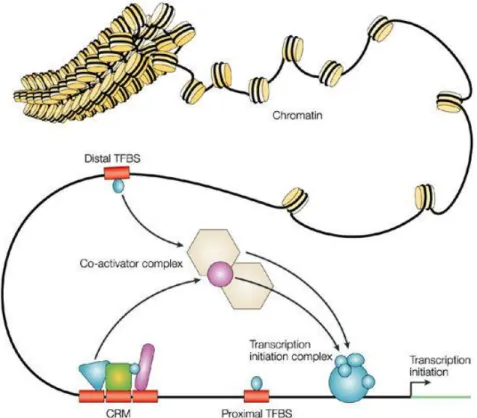
A working model is that transcription factors bind to specific DNA motifs, but still these appear to have some wobble, allowing for some flexibility in binding (Herr and Cleary, 1995). These transcription factors recruit a co-activator complex to the DNA binding site and stabilise the transcription initiation complex at the promoter. Where this site is near the promoter of a gene, the transcription factors and mediator proteins are able to recruit RNA polymerase to initiate transcription. Sets of transcription factors can bind in co-localised regions known as cis-regulatory modules. These combinations can allow specific regulatory instructions for the nearby genes, influencing spatial-temporal transcription throughout development (Maeda and Karch, 2011) (Figure 4).

(29)

Figure 4. Regulation of gene expression by transcription factors

Adapted by permission from Macmillan Publishers Ltd: [Nature Reviews. Genetics] (Wasserman and Sandelin, 2004), copyright (2004)

Distal elements much further away from the transcription start site can act as gene regulatory elements: enhancers, insulators and silencers (Riethoven, 2010). This genomic regulation by distal transcription binding factors utilises the looping of the DNA and its 3D structure to bring distant acting enhancers close to the transcription start site in order to influence gene expression (Visel et al., 2009b). These are referred to as cis-regulatory elements or modules as they act on genes on their own

chromosome. Understanding when these elements are active, what genes they act upon and even what sequence specific language or grammar they use to do so is the next vast frontier of genomics.

1.2.1.1 Conservation

One method of identifying developmental cis-regulatory elements is through

(30)

phylotypic stage in development, and the genes involved are essentially the same (Duboule, 1994, Raff, 2012). Therefore vertebrate-specific development is likely to utilise the same gene regulatory elements to control this process, with the sequence highly conserved amongst vertebrate species (Woolfe et al., 2005). Sequence conservation is most easily detected using BLAST (Altschul et al., 1990) or BLAT (Kent, 2002) software, however both of these algorithms require high identity thresholds when searching whole genomes for short sequences to obtain significant alignments. There are variations that have been developed for searching whole genomes against each other, such as MegaBLAST (Zhang et al., 2000), that makes this

comparative genomics feasible and identification of large sets of non-coding sequence conservation possible (Lee et al., 2010) (Doglio et al., 2013).

Comparisons of vertebrate genomes, and specifically Fugu-human alignments (Aparicio et al., 1995) show ancient vertebrate conservation of stretches of non-coding DNA with the Fugu genome used due to its highly compact size (Brenner et al., 1993). These highly conserved non-coding elements cluster around vertebrate specific

developmentally important genes (Woolfe et al., 2005). The concept that these stretches of non-coding DNA would stay near-identical throughout such a large evolutionary period suggests that variation and mutation in them would be detrimental to the organism, in a similar way that the coding genome is resistant to random mutation events due to the chance of them being disadvantageous (Drake et al., 2006) (Katzman et al., 2007). Therefore sequence comparisons are able to be utilised to identify human cis-regulatory elements (Prabhakar et al., 2006). These cis-regulatory elements

identified through sequence comparisons are several hundred bases in length, therefore identification of the functional motifs within them is the next step to annotating the non-coding genome. Work has already begun to understand this cis-regulatory logic (Li et al., 2010) and more functional assays of non-coding regulatory elements are necessary to feedback into these computational predictors.

1.2.1.2 Transcription Factor Binding Sites

Sequence-specific DNA binding proteins (transcription factors) are the essential proteins utilised by cis-regulatory elements to regulate gene expression (Latchman,

(31)

1997, Chen and Rajewsky, 2007). Therefore, predicting and identifying the specific DNA motifs, or transcription factor binding sites (TFBS) could help identify cis-regulatory elements and even tissue-specific function. Computational methods have been implemented to do this (Ellrott et al., 2002) but often the number of identified sites is much greater than the number able to be functionally validated. This is made even more complex by the ability for these transcription factors to identify motifs with some ‘wobble’ – the exact motifs may vary by a handful of bases in some instances, the TFBS can be seen as a ‘preference’ rather than an exact sequence (Badis et al., 2009). For example, the JASPAR database (Mathelier et al., 2016) collates models of

transcription factor binding sites in various species based on position frequency matrices (Figure 5).

Figure 5. An example of JASPAR database information for FOXD1 TFBS (Mathelier et al., 2016).

A key method in identifying binding sites is through capturing transcription factor binding events in vitro. Thanks to advances in sequencing, this combined with

chromatin immunoprecipitation has allowed genome-wide ChIP-Seq to identify protein-DNA interactions (Valouev et al., 2008). Using transcription factors as ‘bait’ in these assays, binding events are captured and the sequences involved can be analysed for common motifs. This can be used to predict enhancers themselves (Schmidt et al., 2010, Visel et al., 2009a) as well as provide further TFBS information. The method relies on

(32)

crosslinking of transcription factors and DNA followed by using factor-specific antibodies to pull down the regions bound and detect individual binding events. Genome-wide, this one versus all method can describe a footprint of the transcription factor across the genome, and utilising a cell- or tissue-specific approach can help identify cell- or tissue-specific enhancers (Blow et al., 2010). Despite these benefits, this approach does struggle to distinguish between genuine functional binding events and those that do not instigate downstream events. Therefore, there is a high false-positive rate (Nix et al., 2008, Pickrell et al., 2011) and often the number of peaks is far too high to then functionally assay. Some progress has been made to reduce this, including comparisons of multiple TFBS peaks for common regions that could

contribute to cis-regulatory modules (Zinzen et al., 2009). Crucially, understanding the specificity of transcription factor binding sites will be essential in elucidating the role a single nucleotide polymorphism could play within an evolutionary identified enhancer.

1.2.1.3 DNA-DNA interactions

Our understanding of the coding regions of the genome comes from the linear sequence of nucleotides, however the three-dimensional organisation of the chromatin has a part to play in gene regulation, bringing regions of the genome millions of bases away to close proximity in the nucleus. We are now able to capture these long-range interactions thanks to advances in a technique called chromosome conformation capture (Cope and Fraser, 2009). Crosslinking of DNA-DNA interactions and subsequent sequencing of the fragments involved allows the identification of loops and structural folding (Figure 6).

(33)

Figure 6. Chromosome conformation capture (3C) technique overview.

The interacting loci are cross-linked, capturing long range interaction. The DNA is restriction-enzyme digested and the fragments are then ligated. This occurs in dilute conditions to allow for preferential ligation to close-proximity strands. The DNA is then purified and various sequencing techniques are used to identify the interacting regions.

The chromosome conformation capture technique has evolved rapidly over the past decade, initially utilising PCR sequencing for a ‘one vs one’ viewpoint of interactions (Dekker, 2006). This is useful for confirming interactions between two regions.

Alternatively the 4C approach of ‘one vs all’ (Simonis et al., 2006) allows a promoter or enhancer region to be used as a viewpoint and captures all potential interactions. This is particularly useful for identifying cis-regulatory elements for a specific gene, or the genes a cis-regulatory element might act upon. A recent iteration, Hi-C (Lieberman-Aiden et al., 2009) is an ‘all vs all’ high throughput sequencing approach that has since been extensively used across the whole human genome and led to the definition of topologically associating domains. Mapping these long-range interactions reveals how the human genome folds on itself and creating functionally important loops

(Lieberman-Aiden et al., 2009).

Recently, evidence has shown that the underlying organisation of genomic regions can be mapped to approximately 100kb to 1mb of locally interacting DNA known as topologically associating domains (TADs) (Dixon et al., 2012). Utilising TAD information may help understand how non-coding regions affect gene regulation, as

(34)

enhancers within the same TAD as a specific gene are much more likely to act on that gene than one potentially closer but in a different TAD.

Topologically Associating Domains have been shown to have limited change when compared across species and cell types (Dixon et al., 2012, Nora et al., 2012) with key changes in chromatin architecture reorganisation in differentiating stem cells (Dixon et al., 2015). Some evidence has shown their involvement in facilitating transcriptional regulation through the integration of regulatory activities within their boundaries (Nora et al., 2013). TADs bring together the genes and cis-regulatory elements to allow cell-specific gene expression patterns characteristic of phenotypes observed (Sanyal et al., 2012). As the majority of GWAS variants are found in the non-coding genome

(Manolio et al., 2009), utilising the information from TAD boundaries may help assign the correct gene these variants are acting on if found at TAD boundaries. In addition, disruption of TAD boundaries has been shown to form de novo enhancer-promoter interactions, gene mis-expression and resulting abnormal phenotypes (Lupiáñez et al., 2015).

A key limitation to these techniques is the resolution of interactions they obtain, mostly limited by the enzyme digestion and the sequencing depth. With deep sequencing, restriction fragment length resolution is possible with Hi-C (Jin et al., 2013, Rao et al., 2014), allowing mapping of interactions to ~1kb in cell lines. However, enhancers can often be much smaller than that and binding sites within them even smaller so.

Therefore 3C, 4C and Hi-C methods all have their benefits but do not reveal the single nucleotide level of sequence contribution to cis-regulatory elements. Many different models are now developing to resolve how the TADs shape the 3D architecture of the genome and drive the networks of cis-regulatory elements that determine gene

expression during development (Remeseiro et al., 2016).

1.2.2 Human non-coding variation

Within the non-coding genome, natural human variation can occur and this is markedly more often than in the exome due to the functional constraint on the sequences that transcribe proteins (Genomes Project Consortium, 2010). Since the initial 1000

(35)

Genomes data release, the third release (The Genomes Project, 2015) has presented with more opportunity to interrogate the noncoding genome for rare variants thanks to an improvement in coverage. Any individual is thought to carry 3.5-4.5 million SNPs across their whole genome, with individuals of African ancestry having the most (The Genomes Project, 2015). Therefore, any attempt to find function in the variation of the non-coding genome is met with a vast number of variants with limited information. Reducing the region of the non-coding genome to be interrogated through functional annotation of regulatory elements allows more reasonable analysis. Previous

comparisons of percentage of sites containing SNPs across the non-coding genome compared to the coding sequence consistently show higher frequencies of variants in the non-coding. When comparing variation in CNEs, this shows these sequences are

constrained to a similar level to non-synonymous coding variants (De Silva et al., 2014). Evidence shows that these CNEs are selectively constrained and not just mutational cold spots that have been retained over evolution (Drake et al., 2006). Outside of non-coding regulatory elements there is a large potential for genetic variation with no noticeable phenotypic effect. However there is also the potential for

accumulation of mutations in the non-coding genome to influence continuous traits such as height (Lango Allen et al., 2010). The extent of non-coding regulatory variation and its contribution to evolution and natural selection is unclear (Lappalainen and

Dermitzakis, 2010). However if gene regulation can be affected incrementally through regulatory variation, it gives the potential for smaller phenotypic variations to

accumulate and, if beneficial, be positively selected for evolutionary. The converse could also be true if small genetic variation in regulatory elements is able to have just as severe an impact on phenotype as a nonsynonymous mutation.

1.2.3 Contribution to human disease and disorders

Most disease-associating variants that have been found in GWAS studies are located in the non-coding region of the genome (Maurano et al., 2012). Often these variants correlate to relatively small increments in risk in complex human diseases and traits (Manolio et al., 2009). There have been some examples of non-coding variation being the fundamental cause of a developmentally based disorder. A key example that also demonstrates the vast distances that gene enhancers can act across is a set of mutations

(36)

in the ZRS regulatory element that acts on the Shh gene (Lettice et al., 2003). Four unrelated families with congenital polydactyly were found to have point mutations within the ZRS, affecting the Shh expression in the ZPA. Since this evidence of such a strong effect of a SNP at such a large distance (~1Mb), further efforts to provide

evidence for non-coding SNPs to be causative of human disease have gained traction. The use of 4C-seq analysis have shown that a common functional variant in a cardiac enhancer modulates cardiac SCN5A expression, predisposing patients to arrhythmia (van den Boogaard et al., 2014). Another approach has shown that gestational

hyperglycaemia associating haplotypes disrupt regulatory element activity of the nearby HKDC1 gene, altering glucose homeostasis (Guo et al., 2015). The Deciphering

Developmental Disorders project estimates that 42% of their cohort may have

pathogenic mutations in the coding regions of the genome (Deciphering Developmental Disorders, 2017) and although the other half of the cohort may not be diagnosed

through non-coding mutations, it is fair to predict that some of these cases may be explained this way. It is difficult to tell if multiple variants, both in the coding and noncoding regions may contribute to developmental disorders and much of the functional analysis of non-coding variants is yet to be done. In many instances,

associating variants to disease phenotypes is possible, as is associating them to familial inherited disorders, however proving their effect on gene expression can be far more complex and time consuming.

1.2.4 Noncoding variation functional prediction

Noncoding variants can be pathogenic and they are also found at a higher rate than coding variants. Therefore, a great deal of resource has been put into computational methods to predict non-coding variant function and pathogenicity. This is made particularly difficult as many regulatory elements are predicted themselves based on sequence conservation, transcription factor binding sites, and chromosome

conformation capture methods (see above: 1.2.1.1, 1.2.1.2, 1.2.1.3). Regulatory SNVs can affect histone modification, DNA methylation, and TF binding and all to various extents. The effect of these SNVs is very much unknown and we must rely on

prediction models to sift through the vast number of personal and associating SNVs to find pathogenic variants.

(37)

Computational methods of scoring pathogenicity variants rely on available functional data sets to complement these predictors. As mentioned previously, comparing PWMs between normal and variant versions of a locus may help judge the change in putative binding affinity that a variant imposes. Utilising public databases such as TRANSFAC (Matys et al., 2003), JASPAR (Mathelier et al., 2016) and UniPROBE (Hume et al., 2014) can give these scores and their changes (Bailey et al., 2009) and predict pathogenicity based on changes in transcription factor binding. Methods such as the transcription factor affinity prediction (TRAP) utilises ChIP-seq peaks to determine the highest binding affinity transcription factors and then gives mutated sequence p-values for changes in binding sites (Thomas-Chollier et al., 2011). Much of the prediction of effect is reliant on a collection of know transcription factors and their binding sites, and is therefore limited by functional assays to feed in more information.

Further improvements to the functional prediction of SNVs can be made by integrating more publicly available experimental data, such as that of ENCODE (ENCODE Project Consortium, 2007). This uses DNaseI-hypersensitive sites (DHS) and histone

modifications to predict regulatory elements. As short TFBS sequences (6-20bp

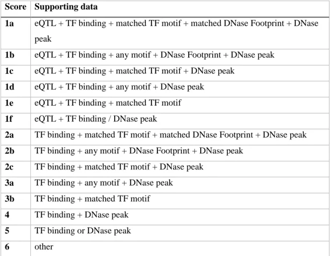
generally) can be found in a large proportion of the genome, finding variants that are in active regulatory elements are more likely to be pathogenic than those in inactive regions. A database that utilises chromatin states alongside transcription factor binding (both motifs and experimentally validated data) is RegulomeDB (Boyle et al., 2012). This combines information on histone modifications, DHS, TF binding, TF motifs and conservation to score variants in categories related to predicted functional consequences (Table 1). This integration of data and emphasis on expression quantitative trait loci (eQTLs) helps to identify active regulatory elements. The eQTLs are regions of the genome shown to have an influence on gene expression level however these

experiments are costly both financially and in time and therefore unable to be used for all possible variation found. In addition, RegulomeDB is somewhat limited by the known human genetic variation, currently using dbSNP build 141 (Sherry et al., 1999, Sherry et al., 2001). Its output is easily interpreted and compared across cohort groups, or case-control studies.

(38)

Table 1. RegulomeDB scoring categories for SNPs

Score Supporting data

1a eQTL + TF binding + matched TF motif + matched DNase Footprint + DNase peak

1b eQTL + TF binding + any motif + DNase Footprint + DNase peak 1c eQTL + TF binding + matched TF motif + DNase peak

1d eQTL + TF binding + any motif + DNase peak 1e eQTL + TF binding + matched TF motif 1f eQTL + TF binding / DNase peak

2a TF binding + matched TF motif + matched DNase Footprint + DNase peak 2b TF binding + any motif + DNase Footprint + DNase peak

2c TF binding + matched TF motif + DNase peak 3a TF binding + any motif + DNase peak

3b TF binding + matched TF motif 4 TF binding + DNase peak 5 TF binding or DNase peak 6 other

An additional method to evaluate the effect of a single base change is to look at the precise genomic location conservation over evolution. This is particularly useful when looking at variants associating with developmental disorders as regulation of vertebrate-specific development appears to be conserved between species (Piasecka et al., 2013) and by conserved regulatory elements (Woolfe et al., 2005). However, within these conserved noncoding elements there is some variation in individual bases despite the high overall consensus sequence. Individual nucleotides can be in non-variable or restricted variable regions (NVRs or RVRs) (De Silva et al., 2014). The base-by-base conservation, and the probability of a variant to be pathogenic as a result, can be scored using a database like GERP++ (Davydov et al., 2010). GERP++ uses rejected

substitutions and neutral rate of mutation over evolution to give base-wise scores of variants based on alignments and a model of neutral evolution. The limitations of GERP++ and other similar approaches arises from the neutral rate of mutation

(39)

estimations. They are often uncertain and can vary dependent on the alignment quality, methodology used to estimate them and the genomic region. In addition, these methods make the assumption that all sites in the sequence region are independent.

Further computational methods attempt to integrate more data for large-scale annotations and scoring. One of that is widely used is the Combined Annotation Dependent Deletion software (CADD) (Kircher et al., 2014). This software integrates multiple annotations and contrasts variants with simulated mutations and known common human variation. Machine learning software like CADD allows easy scoring of variants and ranking within a cohort set. It utilises 88 annotations from genomic and epigenomic data sets covering conservation, transcription factor binding, cell expression levels, chromatin states and histone modifications. It utilises the variant effect predictor (VEP) from ensembl (McLaren et al., 2016) for annotation as well as ENCODE data. CADD has been shown to be a valuable tool for noncoding annotation (Richardson et al., 2016) but some questions over its clinical validity remain (Mather et al., 2016). Some of the difficulty in scoring noncoding variants using CADD may result from its machine learning approach and training data that also contains coding variants. Some unsupervised approaches of integrating the same amount of annotations and scoring have also been developed (Ionita-Laza et al., 2016) with the latter more preferable in the absence of a large, representative and correctly labelled training set. CADD is able to readily integrate new information, and its upkeep in light of continued ENCODE annotation releases is a crucial benefit. The key addition to noncoding variant

annotation will be tissue specific eQTLs and expression analysis, especially in light of human disease and phenotypes. However, these methods can only prioritise variants based on predicted functionality. This is a necessary step to reduce the number of variants to be functionally validated and both time and cost prevent all from being investigated. Once functional validation has been carried out, it is imperative that this information is fedback into these predictive models to continually improve their accuracy. This limiting step of validation is one of the key roadblocks in determining noncoding variation function.

(40)

1.2.5 Noncoding variation functional validation

Functionally validating noncoding variants is dependent on prior knowledge or hypothesis of how these variants function. Functional validation could be defined as showing that a genetic variant has a cause and effect relationship, affecting gene function, expression or developmental processes. This is developed through the annotation tools mentioned above (1.2.4). There are various methods that can be used to assess a variant’s effect on gene expression and potentially phenotype including luciferase assays (Ozaki et al., 2002), allele-specific FAIRE assays (Smith et al., 2012), transient enhancer assays (Bessa et al., 2009), dual-reporter transgenesis (Bhatia et al., 2015), and CRISPR-Cas9 mutagenesis (Canver et al., 2015). Many of these methods are low-throughput, or the ones that are high-throughput reply on relevant cell lines and are not necessarily able to translate to the whole organism. This is particularly true for developmental enhancers, such as those predicted by conservation, and in vivo methods are more likely to give better evidence to the effects of a regulatory SNP on the

developing embryo than in vitro methods. Conversely, in vitro methods may give a better understanding of the effect of a variant at the molecular level, such as

transcription factor binding.

In vitro methods to quantify the effect of a SNV on DNA-protein interactions have been used previously to confirm non-coding variant effects in GWAS identified variants (Oldoni et al., 2016). Allele-specific formaldehyde-assisted isolation of regulatory elements (FAIRE) can show binding differences between wild-type and variant regulatory elements but gives limited information in regards to the transcription factor binding that changes and is reliant on cell-type specific nuclear extract. Luciferase reporter assays allow quantification of the changes in enhancer-driven gene expression between variants, but are again limited by appropriate cell lines and the lack of whole-organism information. These assays are fundamental as proof of concept and have been developed to be high throughput and quantitative (Smith et al., 2012, Melnikov et al., 2012).

An additional method of interrogating the relationship between a putative enhancer and gene regulation is the visualisation of a reporter gene under the control of the element in

(41)

vivo. The core principal that an enhancer can drive a minimal promoter underpins much of the in vivo enhancer assay used. This includes lacZ assays such as those in the

extensive VISTA enhancer catalogue in mice (Visel et al., 2006) and the Tol2:GFP transposon mediated approach in Zebrafish (Kawakami, 2007). In addition, stable zebrafish transgenic lines using allele-specific enhancer-reporter constructs for the regulatory region of interest can show differences in in vivo function, although these can be hard to detect and are very low-throughput (Liu et al., 2017). The benefits of

transient enhancer assays in Zebrafish come from the medium-throughput approach (multiple constructs can be analysed in a week) as long as the disease the variant associates with is developmentally relevant. Nevertheless, the mosaicism that can occur from random integration of the expression construct can make it difficult to find tangible evidence of a variant’s effect between microinjections. Therefore, it is

paramount to do multiple repeats, and some work has been performed to utilise dual-colour assays to allow an all-in-one approach, removing variation between injections (Bhatia et al., 2015). Therefore, there is a fine balance to be met between high-throughput and less reproducible analysis and low-high-throughput but highly accurate experiments.

One method of reliably assessing the function of a regulatory element variant in relation to a disease phenotype would be to create a comparable mutation in an animal model. Thanks to the advancement of CRISPR-Cas9 technology (Ran et al., 2013), the ability to mutate allele-specific sites anywhere in the genome is possible. For regulatory elements that have been discovered through comparative genomics, such as

evolutionary conserved developmental enhancers, this method can be suitable as the DNA surrounding a regulatory variant is likely to be identical in human and in the vertebrate model being used. This genome-editing is costly and time consuming and therefore strong prior evidence of the variant’s function must be observed, however resulting phenotypes can be verified, as well as changes in gene expression (Han et al., 2015). This single-base interrogation of regulatory elements will not only give insights into the downstream effect of a variant but also feed back into the field’s computational predictions of SNV effects and help understand the language and grammar of the noncoding genome. Conversely, this approach does not take into consideration the

(42)

environment-genome interactions and the part they play in complex hereditary diseases. As it is expected that multiple noncoding variations and their accumulation are more likely to affect gene regulation due to combined effects (Cannavò et al., 2016) combinations of mutations may need to be implemented to fully understand the threshold for a disease phenotype from noncoding variation. This information will ultimately shape the way we search for noncoding variants and predict and validate their impact, in an attempt to consolidate the vast amount of sequence information we are currently producing.

(43)

Chapter 2. Materials & Methods

2.1 Methods for Chapter 3: Obesity project

2.1.1 Sequencing

Samples were curated and individuals were assessed as described previously (Klöting et al., 2008). Libraries were prepared for sequencing using Illumina Nextera Rapid

Capture Custom Enrichment Kit (Cat ID FC-140-1009). The custom kit included 8,701 probes across the 2 Mb region for 288 samples (Project ID 44309). All samples were run on an Illumina HiSeq 2500 at 100 cycle pair end reads. Ninety-six multiplexed samples were run per flow cell with each multiplex being run twice on Rapid Run mode. Samples were de-multiplexed and converted to FASTQ files using Illumina software CASAVA.

2.1.2 Ethical statement

The study was approved by the regional scientific ethics committee and by the Danish Data Protection Board and fulfilled the Helsinki Declaration.

2.1.3 Availability of supporting data

Sequence data (reads) are be available through ENA at http://www.ebi.ac.uk/ena. Accession number PRJEB11794. All other data are contained within the paper or supplementary information files. All other data is fully available on request, without restriction.

2.1.4 Mapping and variant calling

Sequencing data (FASTQ) files was mapped to the hg19 assembly of the human genome, the version in human_g1k_v37.fasta file available from the 1000 Genomes Project (ftp://ftp.1000genomes.ebi.ac.uk/vol1/ftp/technical/ reference/). BWA (Burrows-Wheeler Aligner) software was used to map the reads (Li, 2013), version bwa-0.7.8, bwa-mem algorithm with default parameters. The mapped read (sam) files were then converted to bam format using samtools version 0.1.19 (Li et al., 2009a). The

(44)

Chapter 2 Materials and Methods

reads in each bam file were then sorted by chromosome and coordinate and indexed using samtools.

Duplicate reads were marked by Picard (http://broadinstitute.github.io/picard), version 1.91, MarkDuplicates tool. Then the two bam files from different sequencing runs for each individual were merged using Picard tool MergeSamFiles. The individual bam files per sample were then processed by our in-house tool ‘TidyVar’ (B. Noyvert and G. Elgar, manuscript in preparation, https://github.com/boris-noyvert/TidyVar.m), which is an implementation of a novel variant calling algorithm. The algorithm uses a string matching approach to detect SNPs and short insertions and deletions, the individual genotypes are assigned using pattern recognition. A single vcf file listing all the variants found in all the individuals was produced.

2.1.5 Haplotype analysis

Haplotyping was performed with Haploview (Barrett et al., 2005) using the methods described previously for defining linkage disequilibrium blocks (Gabriel et al., 2002). For this programme, only biallelic SNPs were used across the region chr16:53,500,000-55,500,000. Comparisons over each variant over 500Kb were performed and settings altered from default to ignore Hardy-Weinberg P values, and to include only individuals with a minimum of 75% of all SNPs successfully called. Associations of individual variants and haplotypes were produced through Haploview using the case-control allelic chi-squared test with one degree of freedom for the 2 × 2 contingency table of allele counts for reference and non-reference alleles and for case and control separately (Clarke et al., 2011). The output P-values of this were used throughout this study.

2.1.6 Interaction data liftOver

The UCSC genome browser utility liftOver (http://geno

me.ucsc.edu/cgi-bin/hgLiftOver) was used as the Batch Coordinate Conversion method to transfer SNP hg19 coordinates to mouse genome build mm9 coordinates using default settings. Conversion of 5,842 SNPs was successful with 5,988 SNP locations failing.