Multivariate generalized S-estimators
o
E. Roelant, S. Van Aelst and C. Croux
DEPARTMENT OF DECISION SCIENCES AND INFORMATION MANAGEMENT (KBI)
Multivariate Generalized S-estimators
Roelant E.
a,∗
Van Aelst S.
aCroux C.
baDepartment of Applied Mathematics and Computer Science, Ghent University
-UGent, Krijgslaan 281-S9, B-9000 Gent, Belgium
bKatholieke Universiteit Leuven, University Centre of Statistics, Naamsestraat 69,
B-3000 Leuven, Belgium
Abstract
In this paper we introduce generalized S-estimators for the multivariate regression model. This class of estimators combines high robustness and high efficiency. They are defined by minimizing the determinant of a robust estimator of the scatter matrix of differences of residuals. In the special case of a multivariate location model, the generalized S-estimator has the important independency property, and can be used for high breakdown estimation in independent component analysis. Robustness properties of the estimators are investigated by deriving their breakdown point and the influence function. We also study the efficiency of the estimators, both asymptotically and at finite samples. To obtain inference for the regression parameters, we discuss the fast and robust bootstrap for multivariate generalized S-estimators. The method is illustrated on several real data examples.
Key words: Bootstrap, efficiency, multivariate regression, robustness.
∗ Corresponding author. Tel.:+32-92644756; fax: +32-92644995
1 Introduction
In this paper we introduce a new class of estimators for the multivariate regres-sion model, called Generalized S-estimators (GS). Generalized S-estimators are defined by minimizing the determinant of a robust estimator of the scat-ter matrix of differences of residuals. Using differences instead of the residuals themselves has several advantages. First of all, at most models this will lead to an increase in statistical efficiency, while the robustness of the estimators, as measured by their breakdown point, remains the same. The breakdown point of an estimator is the highest possible percentage of outliers than an estimator can withstand. It turns out to be possible to achieve the highest possible value for the breakdown point, 50%, even when working with differences of resid-uals. A second advantage is that GS-estimators allow to estimate the slope and the scatter matrix of the error terms of the multivariate regression model, without needing to estimate the intercept. Hence, the estimation procedure is “intercept free.”
The multivariate regression model encompasses both the multivariate location-scale model, as a multivariate regression model with only an intercept, and the univariate regression model. While GS-estimators were already consid-ered for univariate regression (Croux et al. 1994), they were not studied yet for the multivariate location-scale model. In the latter model, the “intercept free” property of the GS estimator translates into “location free” estimation. Hence, GS-estimators allow for estimation of scatter while not needing to esti-mate the location. Moreover, since the GS-estimator is based on differences, it has the independence property, meaning that when the components of a ran-dom vector are independent, the scatter matrix estimate is diagonal (Tyler et
al. 2007). This is not true for S-estimators of scatter in general. The indepen-dence property is highly important in independent component analysis (ICA). Briefly, the ICA problem consists of finding an original random vector with independent components when only an unknown linear mixture is observed (Hyv¨arinen et al. 2001). Oja et al. (2006) proposed a method for ICA that is based on the use of two different scatter matrices that are required to have the independence property; see also Tyler et al (2007). By using the GS-estimator, a high breakdown approach to robust ICA is obtained. Other scatter matrix
estimators, based on differences of observations were proposed by D¨umbgen
(1998), and Sirki¨a et al. (2007). They are of the M-type and their breakdown
point decreases with the dimension (D¨umbgen and Tyler 2005), and thus do
not have a high degree of robustness.
Consider the multivariate linear regression model given by
y=α+BTu+ǫ (1)
whereuis thep-variate predictor,ythe q-variate response and ǫtheq-variate
error term which has center zero and a positive definite scatter matrix Σ.
The unknown parameters θ = (α,BT)T ∈ R(p+1)×q and Σ ∈ Rq×q are to be
estimated from the observations Zn = {zi := (xTi ,yTi )T = (1,uTi ,yTi )T, i =
1, . . . , n} ⊂Rp+q+1. The classical estimator for this model is the least squares estimator, but it is well known that this estimator can be highly influenced by outliers.
In the univariate regression case a lot of research has been done to con-struct more robust estimators. Classes of robust estimators in this setting include M-estimators (Hampel et al. 1986), least median of squares and least trimmed squares estimators (Rousseeuw 1984), S-estimators (Rousseeuw and
Yohai 1984), MM-estimators (Yohai 1987), CM-estimators (Mendes and Tyler
1996) and τ-estimators (Yohai and Zamar 1988). Croux et al. (1994)
intro-duced a class of regression estimators, called generalized S-estimators or GS-estimators. While an S-estimator of regression minimizes an S-estimator of scale of the residuals, a GS-estimator minimizes an S-estimator of scale ap-plied on the pairwise differences of the residuals, instead of on the residuals themselves. It has been shown that for bounded loss functions these univariate GS-estimators have nice properties such as a high breakdown point, a higher efficiency than the original S-estimators. Moreover, they do not require the assumption of asymmetric errors (see also H¨ossjer et al. 1994, Berrendero and Romo 1998 and Berrendero 2002). In this paper, we extend the definition of GS-estimates to multivariate regression.
Recently, several robust estimators for multivariate regression have been in-troduced. Methods based on robust estimators for multivariate location and scatter applied to the joint distribution of responses and explanatory vari-ables have been proposed by Ollila, Oja and Hettmansperger (2002) using sign covariance matrices, Ollila, Oja and Koivunen (2003) using rank covari-ance matrices and Rousseeuw et al. (2004) using the minimum covaricovari-ance determinant estimator. An alternative approach is to define a robust regres-sion estimator by minimizing a robust estimate of the covariance matrix of the residuals. Agull´o et al. (2008) proposed the multivariate least trimmed squares estimator, Van Aelst and Willems (2005) considered multivariate regression
S-estimators, while Ben, Martinez and Yohai (2006) introduced τ-estimators
for multivariate regression. All these procedures, however, are not based on differences of residuals, and are not intercept or location free.
intro-duce the multivariate regression GS-estimators and determine their breakdown point. Section 3 describes the algorithm for computing the GS-estimators. In Section 4 we define the functional form of the estimator. We show that the GS-functional is Fisher-consistent if the differences of the errors have an ellip-tical distribution. We also derive the influence function of the GS-functional. Asymptotic variances and corresponding efficiencies are given in Section 5. Section 6 discusses the fast and robust bootstrap method for GS-estimators. Section 7 presents two real data examples and Section 8 concludes. All the proofs can be found in the Appendix.
2 Definition and breakdown point
We now define Generalized S-estimators for the multivariate regression model given in (1).
Definition 1 Let Zn = {zi := (xTi ,yiT)T = (1,uTi ,yTi )T, i = 1, . . . , n} ⊂
Rp+q+1. The GS-estimates of multivariate regression(Bbn,Σbn)minimizes among
all (B, C) ∈ Rp×q ×P DS(q), with P DS(q) the set of positive definite
sym-metric q×q matrices, the determinant |C|, subject to the condition à n 2 !−1 X i<j ρ([(ri−rj)TC−1(ri −rj)]1/2) =k (2) where ri =yi−BTu i−α.
Note that the objective function does not depend on the intercept α. The
constantkcan be chosen ask =EF×F[ρ(kǫ1−ǫ2k)], which ensures consistency
at the model with error distribution F (see Section 4). The choice ρ(u) = u2
we impose the following properties on the loss function ρ:
• ρ is symmetric, twice continuously differentiable and ρ(0) = 0
• ρ is strictly increasing on [0, c] and constant on [c,∞) for somec < ∞.
Throughout this paper we use the well-known class of Tukey biweight ρ
-functions given by:
ρc(t) = t2 2 − t4 2c2 + t 6 6c4, |t| ≤c c2 6, |t| ≥c
Similarly as in Lopuha¨a (1989), it can be shown that definition 1 implies that multivariate GS-estimators satisfy the following first-order conditions:
X i<j u(dij)(ui−uj)(yi−yj −BT(ui−uj))T =0 (3) X i<j {qu(dij)(yi−yj−BT(ui−uj))(yi−yj−BT(ui−uj))T −v(dij)C}=0 (4) withd2 ij = (yi−yj−BT(ui−uj))TC−1(yi−yj−BT(ui−uj)),u(t) =ψ(t)/t and v(t) = ψ(t)t−ρ(t) +k, where ψ(t) = ρ′(t).
To study the global robustness of the multivariate GS-estimators, we derive
their finite-sample breakdown point. For a given data setZn, the finite-sample
breakdown point ǫ∗
nof an estimatorTn is the smallest fraction of observations
of Zn that need to be replaced by arbitrary values to carry the estimate Tn
beyond all bounds (Donoho and Huber 1983). Formally, ǫ∗ n(Tn,Zn) = min ( m n; supZ′ n kTn(Zn)−Tn(Zn′)k=∞ )
where the supremum is over all possible collections Z′
n that differ from Zn
the smallest fraction of outliers that can make the first eigenvalue arbitrarily large or the last eigenvalue arbitrarily small. We derive the breakdown point for data sets that satisfy the following general position condition.
Condition 1 The differences of the observations (uTi ,yTi )T are in general
po-sition, meaning that no³p+q2+1´of the differences((ui−uj)T,(yi−yj)T)T with
i < j belong to the same hyperplane in Rp+q.
Note that if the differences of the (uTi ,yTi )T are in general position, then the
points (uTi ,yiT)T themselves are also in general position. The latter means
that no p+q + 1 of the (uTi ,yTi )T lie on the same hyperplane of Rp+q. If
the observations are sampled from a continuous distribution, then condition 1 holds with probability 1.
The breakdown point of multivariate regression GS-estimators, given next, extends the results for the univariate regression case in Croux et al. (1994).
Theorem 1 Let Zn ⊂ Rp+q+1. Denote r := k/sup(ρ). If Zn satisfies
condi-tion 1 and ³n2´(1−r)≥³p+q2+1´ then the breakdown point of the multivariate GS-estimator is given by ǫ∗n(Bbn,Zn) =ǫ∗n(Σbn,Zn) = 1 n min(⌈n−1/2− q 1 + (1−r)(4n2−4n)/2⌉, ⌈1/2−p−q+q1 + (1−r)(4n2−4n)/2⌉).
The maximal breakdown point is achieved for r = 1−((n −1 +p+q)2 −
1)/(4n2−4n), in which caseǫ∗
n =⌈n−p−q/2⌉/n. The asymptotic breakdown
point ǫ∗ = lim
n→∞ǫ ∗
n equals
Taking r = 0.75 yields an asymptotic breakdown point of ǫ∗ = 0.5. Hence, GS-estimators can attain the highest possible value for the breakdown point. In practice, if the GS-estimator needs to achieve a specified breakdown point
ǫ∗, for exampleǫ∗ = 0.5, and to have consistency at a model with error
distri-butionF, typically the normal distribution, the constantcin Tukey’s biweight
function needs to be taken as the solution of 1−q1−EF×F[ρc(kǫ1−ǫ2k)]/(c2/6) =
ǫ∗.
3 Algorithm
The algorithm we propose is anologous to the fast S-algorithm of Salibian-Barrera and Yohai (2006) for univariate regression. For any sequence of values e1, . . . , e˜n, the corresponding scale s is given by the solution of
1 ˜ n ˜ n X i=1 ρ µe i s ¶ =k.
The fast S-algorithm uses local improvement steps (I-steps) to update an initial estimate of the regression coefficients. In our algorithm, the I-steps are based on the scale of the norm of the pairwise differences of the residuals
kri−rjkC = ((ri−rj)TC−1(ri−rj))1/2. The actual algorithm can be described
as follows:
1. Draw N random sub-samples of size p+q. For each sub-sample calculate
the least squares estimate Bb0
m, m = 1, . . . , N, and the corresponding shape
matrix Γb0
m of the residuals, i.e. the covariance matrix Σb0m of the residuals
is rescaled to have determinant equal to 1. Denote the residuals by ri(Bb0
m),
for i= 1, . . . , n.
a. Calculate an approximate solution of equation (2), as sv = v u u u ts2 v−1× X i<j ρ(kri(Bbmv−1)−rj(Bbmv−1)kbΓmv−1/sv−1)/ Ã n 2 ! k
withs0the median absolute deviation of the normskri(Bbmv−1)−rj(Bbvm−1)kbΓvm−1.
b. Determine the weightswij =u(kri(Bbvm−1)−rj(Bbmv−1)kbΓvm−1/sv) and calculate
b Bv
m as the weighted least squares fit based on the differences of the
ob-servations. Compute then Σbv
m =
P
i<jwij(ri(Bbmv−1)−rj(Bbmv−1))(ri(Bbvm−1)−
rj(Bbmv−1))T with corresponding shape estimate Γbvm.
c. Calculate the pairwise differences of the residuals corresponding toBbvm.
d. Repeat steps a, b and c forv = 2, . . . , κ.
Each sub-sample thus yields an improved estimate (Bbκ
m,Γbκm), m= 1, . . . , N.
3. We now select the τ best solutions (e.g. τ = 5) in an efficient way. Form=
1, . . . , τ, we calculate the scale sm =s(kri(Bbmκ)−rj(Bbmκ)kbΓκ
m), m= 1, . . . , τ.
Form ≥τ, we denote byImthe set containing theτ optimal solutions found
after examining the first m candidates, and Am denotes the maximum of
the scales of the solutions in Im. The next solution (Bbmκ+1,Γbκm+1) will be
included in Im+1 if and only if s(kri(Bbκm+1)−rj(Bbmκ+1)kbΓκ
m+1) < Am which is equivalent to 1 ³n 2 ´X i<j ρ(kri(Bbmκ+1)−rj(Bbmκ+1)kbΓκ m+1/Am)< k. (5)
If condition (5) holds, then we compute the scales(kri(Bbκm+1)−rj(Bbmκ+1)kbΓκ m+1)
and we correspondingly update Im and Am to obtainIm+1 and Am+1. If
in-equality (5) does not hold, then Im+1 =Im and Am+1 =Am. Let us denote
(BbB
m,ΓbBm, sBm), m= 1, . . . , τ the τ optimal solutions andsBm their
correspond-ing scales, for m = 1, . . . , τ.
4. Apply further I-steps to each of the optimal solutions (BbB
m,ΓbBm, sBm), m =
1, . . . , τ, until convergence, which yields the fully iterated solutions (BbF
m = 1, . . . , τ, where sF
m = s(kri(BbFm)−rj(BbFm)kbΓF
m). The final estimate is
the solution (BbF
m,ΓbFm) associated with the smallest scale sFm and the
corre-sponding estimate of the covariance matrix of the residuals is obtained as
b
ΣF
m = (sFm)2ΓbFm.
4 Fisher-consistency and influence function
LetHdenote the class of all distributions onRp+q. We define the GS-functional
GS: H → (Rp×q×P DS(q)) as the solution GS(H) = (BGS(H),ΣGS(H)) of
the problem of minimizing |C| subject to
ZZ
ρ([(y1−y2−BT(u1−u2))TC−1(y1−y2−BT(u1−u2))]1/2)dH(z1)dH(z2) = k
among all (B, C) ∈Rp×q×P DS(q) and where zl = (uT
l ,yTl )T for l = 1,2. It
can be easily seen that the resulting GS-functional is affine equivariant. We assume that the following two conditions are satisfied for the distribution H of z= (uT,yT)T in model (1).
Condition 2 We assume that the differences of the errors ǫi−ǫj in model (1)
have a distribution FΣ with density fΣ(x) = g(xTΣ−1x)/
q
|Σ|, with Σ ∈ P DS(q) the scatter matrix. Furthermore, the functiong is assumed to have a strictly negative derivative g′.
Condition 2 requires that the error terms have a unimodal elliptically symmet-ric distribution around the origin. Note that if the error terms are independent and elliptically symmetrically, then the distribution of the differences of the errors remains elliptically symmetric (Hult and Lindskog 2002). We need
result on Fisher-consistency.
Condition 3 For all β ∈ Rp and γ ∈ Rq not both equal to zero at the same
time, it holds that
PH(βT(u1−u2) +γT(y1−y2) = 0)<1−r.
Theorem 2 The functionals BGS and ΣGS are Fisher-consistent estimators
of the parameters Band Σat any model distributionH satisfying conditions 2 and 3:
BGS(H) =B and ΣGS(H) = Σ.
The influence function of a functional T at a distribution H measures the
effect on T of an infinitesimal contamination at a single point (Hampel et
al. 1986). If we denote a point mass distribution at z = (uT,yT)T by ∆
z,
and consider the contaminated distribution Hε,z = (1−ε)H+ε∆z, then the
influence function is given by
IF(z;T, H) = lim ε↓0 T(Hε,z)−T(H) ε = ∂ ∂εT(Hε,z)|ε=0.
Due to affine equivariance of the GS-functional, it suffices to look at model
distributions H0 that satisfy conditions 2 and 3 and for which B = 0, and
Σ =Iq. Denote F0 =FIq and let G be the distribution of u.
Theorem 3 For model distributions H0 verifying the above conditions, the
influence functions of the GS-estimators for multivariate regression at z0 = (uT0,y0T)T are given by
IF(z0;BGS, H0) = [Cov(u)]−1(u0 −EG[u]) ¯ ψ(y0)T β (6) IF(z0; ΣGS, H0) =IF(y0; ΣGS, F0) = 2 γ1 qEF0 " ψ(ky1−y0k)ky1−y0k à (y1−y0)(y1−y0)T ky1−y0k2 − 1 qIq !# +4EF0[ρ(ky1−y0k)−k] γ3 Iq (7) where ¯ ψ(y0) =EF0 " ψ(ky0−y1k) ky0−y1k (y0−y1) # , andβ =EF0×F0 h 1 qψ′(ky1−y2k) + ³ 1− 1q´u(ky1−y2k)i,γ1 =EF0×F0[ψ′(ky1− y2k)ky1−y2k2+(q+1)ψ(ky1−y2k)ky1−y2k]/(q+2) andγ3 =EF0×F0[ψ(ky1− y2k)ky1−y2k].
For the model with only a constant term, the expression of the influence
function of ΣGS is equivalent to the influence function of the symmetrized
M-estimators of multivariate scatter of Sirki¨a et al. (2007). If q= 1, then the
influence function ofBGSis identical to the influence function of the univariate
GS-estimator (see Croux et al. 1994). Since ¯ψ is a bounded function, it can
be seen that the influence function of BGS is bounded in y0 but unbounded
inu0. Hence good leverage points can have a high effect on the GS-estimator,
but bad leverage points will have a bounded influence.
5 Efficiency
The asymptotic variance-covariance matrix of the GS-estimator at the model
distribution H0 can be computed by means of the influence function, as
(see Hampel et al. 1986) where A⊗B denotes the Kronecker product of a (d1×d2) matrix A with a (d3×d4) matrix B, which results in a (d1d3×d2d4)
matrix with d1d2 blocks of size (d3 ×d4). For 1 ≤ j ≤ d1 and 1 ≤ k ≤ d2
the (j, k)th block equals ajkB, where ajk are the elements of the matrix A.
Denoting Σu :=Cov[u], it follows from (6) that
ASV(BGS, H0) = Kpq à diag à EF0[ ¯ψ(y0)⊗ψ¯(y0) T] β2 ! ⊗Σ−u1 ! , (8)
where Kpq is the commutation matrix, a (pq×pq) matrix consisting of pq
blocks of size (q×p). For 1≤l ≤p and 1≤m ≤q the (l, m)th block ofKpq
equals the (q×p) matrix ∆ml which is 1 at entry (m, l) and 0 everywhere else.
From (6) and (8) we find that the asymptotic variance of (BGS)jk is
ASV((BGS)jk, H0) = (Σ−u1)jj
EF0[ ¯ψ(y0)
2
k]
β2 (9)
while the asymptotic covariances, for j 6=j′, are given by
ASC((BGS)jk,(BGS)j′k, H0) = (Σ−1 u )jj′ EF0[ ¯ψ(y0) 2 k] β2
and all other asymptotic covariances (for k 6=k′) equal 0.
Since we assumed, w.l.o.g. due to affine equivariance, that Σu =Ip atH0, we
have that all asymptotic covariances are zero. FurthermoreASV((BGS)jk, H0) =
EF0[ ¯ψ(y0)
2
k]/β2 does not depend on k and j. Hence, we can compute the
asymptotic relative efficiency of the GS-estimator with respect to the least-squares estimator as:
ARE(BGS, H0) =
ASV((BLS)jk, H0)
for all j = 1, . . . , p and k = 1, . . . , q. The asymptotic relative efficiency of a multivariate regression GS-estimator does not depend on the dimension
p or the distribution of the carriers, but only on the dimension q and the
distribution of the errors terms.
Table 1 shows the relative asymptotic efficiencies forH0 a multivariate normal
distribution, and for a multivariate Student distributionsTν with ν = 3 and 8
degrees of freedom. Results are presented for both GS- and S-estimators (see Table 3.1 in Van Aelst and Willems 2005 for the efficiencies of S-estimators), based on a Tukey biweight loss function. The reported values in Table 1 are based on numerical integration of the analytic expression in (9). From Table 1 we see that the efficiencies for the GS-estimator are high for the 25% as well as
for the 50% breakdown point case. For theT3distribution, the GS-estimator is
far more efficient than the least squares estimator. For theT8 distribution the
GS-estimator still outperforms the LS-estimator in higher dimensions. Com-paring the GS-estimator with the S-estimator, we see that using the pairwise differences generally results in a higher efficiency, in particular for the 50% breakdown point estimates.
We also performed a simulation study to investigate the finite-sample efficiency
of the GS-estimator. We generated m = 1 000 random samples with
predic-tors drawn from the multivariate standard normal distribution. The errors were generated from the multivariate normal distribution or from the
mul-tivariate T3 distribution. We considered multivariate regression models with
p+ 1 = 2 and q = 2 and p+ 1 = 5 and q = 5. The matrix (α,BT)T was set
to zero. For each sample we calculated both the S-estimates (including an
Table 1
Asymptotic relative efficiencies for S- and GS-estimators with respect to the LS estimator at normal and Student distributions.
ǫ∗ 25% 50% GS q= 1 q= 2 q = 3 q = 5 q= 10 q= 1 q= 2 q= 3 q = 5 q = 10 Φ 0.818 0.912 0.940 0.974 0.973 0.683 0.719 0.770 0.843 0.923 T8 0.982 1.077 1.103 1.138 1.162 0.798 0.885 0.944 1.031 1.151 T3 1.902 2.061 2.125 2.235 2.342 1.603 1.872 2.070 2.196 2.445 S q= 1 q= 2 q = 3 q = 5 q= 10 q= 1 q= 2 q= 3 q = 5 q = 10 Φ 0.759 0.912 0.951 0.976 0.990 0.287 0.580 0.722 0.846 0.933 T8 0.894 1.059 1.108 1.141 1.162 0.390 0.739 0.897 1.038 1.153 T3 1.738 2.035 2.137 2.222 2.289 0.904 1.601 1.903 2.177 2.140 as nave j,k( d
Var((Bbn)jk)) for j = 1, . . . , p and k = 1, . . . , q, where Var((d Bbn)jk)
is the empirical variance over the m simulated estimates. The finite-sample
relative efficiency is then computed as the inverse of this variance estimate for
the normal distribution, and as ν/(ν −2) divided by the variance estimate
for theTν distribution. Table 2 lists these finite-sample relative efficiencies for
the 25% breakdown S- and GS-estimator for the normal and T3 model. The
finite-sample relative efficiencies are generally slightly lower than the asymp-totic relative efficiencies of Table 1. If we compare the GS-estimator with the S-estimator we see that the relative efficiencies are comparable at the
Table 2
Finite-sample relative efficiencies forBbGS andBbS (25% breakdown) with respect to
the LS estimator at the normal andT3 distribution
n= 30 n= 50 n= 100 n= 200 n=∞ q= 2 0.881 0.901 0.858 0.867 0.912 Φ q= 5 0.797 0.859 0.921 0.941 0.974 GS q= 2 1.809 1.859 1.901 2.025 2.061 T3 q= 5 1.415 1.669 1.861 1.960 2.235 q= 2 0.875 0.901 0.859 0.867 0.912 Φ q= 5 0.798 0.862 0.924 0.945 0.976 S q= 2 1.788 1.838 1.882 2.005 2.035 T3 q= 5 1.407 1.656 1.846 1.943 2.222
GS-estimator are always higher.
6 Robust inference
6.1 Fast and robust bootstrap
We now consider the issue of statistical inference for the regression parameter
B. We use the fast and robust bootstrap procedure introduced by
Salibian-Barrera and Zamar (2002) for univariate regression MM-estimators. The boot-strap principle is to generate a large number of samples from the original data
set, and to recalculate the estimates for each of these resamples. Then, the
distribution, of √n(Bbn− B) can be approximated by the sample distribution
of√n(Bb∗
n−Bbn) whereBbn∗ is the value of the resampled estimator. When there
are outliers present in the data, this method can be expected to be more ac-curate than using the asymptotic variance. However, the standard bootstrap procedure is non-robust, as some bootstrap samples may contain a fraction of outliers that exceeds the breakdown point of the robust estimates, and compu-tationally demanding, due to the high computation time of robust estimators. Both these problems are resolved by the fast and robust bootstrap (FRB) procedure.
For S-estimators in multivariate models, inference based on FRB has been developed by Van Aelst and Willems (2005) and Salibian-Barrera, Van Aelst and Willems (2006, 2008). The FRB procedure computes bootstrap values of
b
Bn without explicitly calculating the actual estimate for each resample. The
FRB gains a considerable amount of computation time by approximatingBb∗
nin
each resample based on a fixed-point representation of the estimator. Because a reweighted representation of the estimator is bootstrapped, the method will be more robust since outliers downweighted in the original sample, will also be downweighted in each resample, regardless the fraction of outliers in each resample.
Suppose that an estimator of the parameter Θ can be represented by a smooth
fixed-point equation g(Θbn) = Θbn, with g depending on n. Then, using the
smoothness ofg, we can calculate a Taylor expansion about the limiting value
of the estimateΘbn:
b
where Rn is a remainder term and ∇g(.) is the matrix of partial derivatives.
Supposing that the remainder term is small, this equation can be rewritten as
√
n(Θbn−Θ)≈[I− ∇g(Θ)]−1√n(g(Θ)−Θ).
Taking bootstrap equivalents at both sides and estimating the matrix [I −
∇g(Θ)]−1 by [I − ∇g(Θb
n)]−1 yields
√
n(Θb∗n−Θbn)≈[I− ∇g(Θbn)]−1√n(g∗(Θbn)−Θbn). (10)
For each bootstrap sample, we can calculate the right-hand side of this equa-tion instead of the left-hand side. Hence, we approximate the actual estimate
in each sample by computing the function g∗ in Θbn and then apply a linear
correction given by [I− ∇g(Θbn)]−1.
We now apply this procedure to the multivariate GS-estimator. We can rewrite the estimating equations (3) and (4) as
b Bn=An(Bbn,Σbn)−1Bn(Bbn,Σbn) b Σn=Vn(Bbn,Σbn) +wn(Bbn,Σbn)Σbn where An(B, C) = X i<j u(dij)(ui−uj)(ui−uj)T Bn(B, C) = X i<j u(dij)(ui−uj)(yi−yj)T Vn(B, C) = ³n1 2 ´ k X i<j qu(dij)(yi−yj−BT(ui−uj))(yi−yj−BT(ui−uj))T wn(B, C) = 1 ³n 2 ´ k X i<j w(dij)
with w(t) = ρ(t)−ρ′(t)t. Write Θ := vec(B) vec(Σ) ,Θbn := vec(Bbn) vec(Σbn) ,
and for any matricesB and C, put
g vec(B) vec(C) := vec(An(B, C)−1Bn(B, C)) vec(Vn(B, C) +wn(B, C)C) .
The expression for the matrix∇g(.) of partial derivatives can be found in the
Appendix.
Now, for a bootstrap sample {((u∗i)T,(y∗
i)T)T, i= 1, . . . , n} we have that g∗(Θbn) = vec(A∗n(Bbn,Σbn)−1B∗n(Bbn,Σbn)) vec(V∗ n(Bbn,Σbn) +w∗n(Bbn,Σbn)Σbn) where A∗
n, B∗n, Vn∗ and wn∗ are the bootstrap versions of the quantities An,
Bn, Vn and wn, that is with (uTi,yTi )T replaced by ((u∗i)T,(yi∗)T)T. Thus,
in order to get the values of √n(Θb∗
n −Θbn) for each bootstrap sample, we
calculate g∗(Θbn), apply the linear correction given by the matrix of partial
derivatives and use approximation (10). We use casewise resampling to gener-ate the bootstrap samples, which means that we draw with replacement from the observations{(uT
i ,yTi )T, i= 1, . . . , n}.
We now focus on confidence intervals resulting from the FRB procedure. We investigate the robustness of the bootstrap confidence interval by deriving
t ∈[0,1], let Q∗
t denote the tth quantile of the bootstrap sample distribution
of T∗ n: Q∗t = min{x: 1 R ×#{T ∗j n ≥x;j = 1, . . . , R} ≤t}
whereR is the number of bootstrap samples drawn. Singh (1998) defined the
upper breakdown point of a statistic as the minimum proportion of asymmetric contamination that can carry the statistic over any bound. The expected upper
breakdown point of the bootstrap quantile Q∗
t is defined as the minimum
proportion of asymmetric contamination that is expected to be able to carry Q∗
t over any bound, where the expectation is taken over the distribution of
drawingR samples with replacement. For the FRB, if we look at the pairwise
differences of the observations in a bootstrap sample, then this sample of
differences must contain at leastpdifferences of two good observations. Hence,
we need in the bootstrap sample at leastcpgood observations such that
³c
p
2
´ ≥
p to obtain at least p differences of good observations among the differences
of the bootstrap sample. An easy calculation yields cp =⌈12+12√1 + 8p⌉. Let
B(n, δ) be the number of distinct non-outlying observations in a resample of
size n, drawn with replacement from a sample of size n with a proportion δ
of outliers.
Theorem 4 Let Zn ⊂Rp+q+1 and assume that the data satisfies condition 1.
Let ǫ∗
n be the breakdown point of a GS-estimate Bbn. Then the expected upper
breakdown point of thet-th fast bootstrap quantile for any regression parameter Bjk, j = 1, . . . , p;k= 1, . . . , q is given by min(ǫ∗n, ǫEn) where
ǫEn = inf{δ ∈[0,1] :P(B(n, δ)< cp)≥t}.
Table 3 lists values for ǫE
Table 3
Expected upper breakdown values for FRB using maximal breakdown GS-estimators
p= 2, q= 1 p= 8, q= 2
n 10 30 50 100 20 30 50 100
Q∗0.05 ǫEn 0.40 0.50 0.50 0.50 0.50 0.50 0.50 0.50
Q∗0.005 ǫEn 0.30 0.50 0.50 0.50 0.40 0.50 0.50 0.50
GS-estimator with maximal breakdown point. Two different quantiles Q∗
0.05
and Q∗
0.005 are considered, which can respectively be used to construct 90%
and 99% percentile confidence intervals. We see that only for the smallest sample sizes the expected upper breakdown point for the FRB is lower than 50%, in all other cases the maximum breakdown point is reached.
We now show that the FRB converges to the same limiting distribution as the distribution of the GS-estimator does. We need the following assumptions on ρ:
(A.1) The following functions are bounded and almost everywhere continu-ous: ρ′(x) x , ρ′′(x) x2 − ρ′(x) x3 , ρ′′′(x) x3 −3 ρ′′(x) x4 + 3 ρ′(x) x5 , ρ ′′(x) and ρ′′′(x) x (A.2) EG×G[ρ ′(d) d (u1−u2)(u1−u2) T]−1 exists.
Theorem 5 Let ρ be a loss function satisfying (A.1). Let (Bbn,Σbn) be the
multivariate GS-estimators and assume that Bbn P
→ B and Σbn P
→ Σ. Then, given that assumption (A.2) is satisfied, the distributions of √n(Bb∗
and √n(Σb∗
n−Σbn) converge weakly to the same limit distributions as those of
√
n(Bbn−B)and√n(Σbn−Σ)respectively, conditional on the firstnobservations
and along almost all sample sequences.
6.2 Simulation results
We investigate the performance of confidence intervals for the regression
co-efficients based on FRB. Simulations were performed for sample sizesn = 30,
50, 100 and 200 for a multivariate regression model with p = 4 and q = 5.
The predictor variables were generated from a multivariate normal
distribu-tion Np(0, Ip). The true value of the parameter B was set to 1p,q, the p×q
matrix having 1 for each entry. We consider the following simulations schemes:
• normal errors: generated from Nq(0, Iq)
• long-tailed errors: generated from a multivariate Student distribution with
3 degrees of freedom (T3)
• vertical outliers: a proportion 1−δof the errors is generated fromNq(0, Iq),
and a proportion δ generated fromNq(5
q
χ2
q,.991q,1,1.5Iq), forδ = 0.15 and
δ = 0.25
• bad leverage points: a proportion 1 − δ of the errors is generated from
Nq(0, Iq), and a proportionδof the responses generated fromNq(−101q,1,10Iq)
with corresponding predictors replaced by predictors generated fromNp(101p,1,10Ip),
for δ = 0.15 and δ= 0.25.
We computed both the 25% and 50% GS-estimators for 1 000 data sets
gen-erated as described above and applied the FRB procedure with B = 1 000
recalculated values (Bb∗
Bootstrap confidence intervals for the components Bjk were constructed
us-ing the bias corrected and accelerated (BCA) method (see e.g. Davison and Hinkley 1997). The bootstrap intervals are compared with confidence intervals
based on the asymptotic normality of the GS-estimator. The latter 100(1−α)%
confidence intervals are of the form
· (Bbn)jk−Φ−1(1− α 2) q b Vjk/n,(Bbn)jk+ Φ−1(1− α 2) q b Vjk/n ¸
where Vbjk denotes the empirical version of the asymptotic variance (EASV)
of the (j, k)-th component of Bbn. The estimates ˆVjk are obtained by replacing
Σ by Σbn, replacingF0 by the empirical distribution of the vectorsΣb−n1/2(yi−
b BT
nui), and finally replacing Σu by the corresponding sample moment.
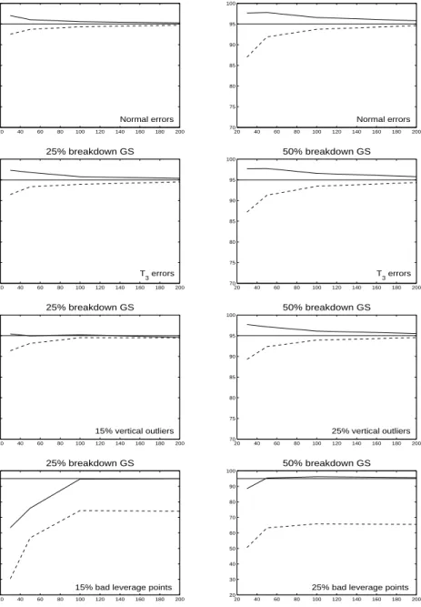
Figure 1 shows the coverage for 95% confidence intervals computed by FRB and EASV. From Figure 1 we clearly see that the coverage of the EASV-based intervals is generally lower than 95%. As the sample size grows, the EASV-based intervals converge to a 95% coverage, except in the case of bad leverage points. The FRB performs better than the EASV method. For small sample sizes the FRB is generally somewhat conservative except for bad leverage points. However, also in that case the coverage converges quickly to 95% when the sample size increases.
20 40 60 80 100 120 140 160 180 200 70 75 80 85 90 95 100 25% breakdown GS Normal errors 20 40 60 80 100 120 140 160 180 200 70 75 80 85 90 95 100 50% breakdown GS Normal errors 20 40 60 80 100 120 140 160 180 200 70 75 80 85 90 95 100 25% breakdown GS T 3 errors 20 40 60 80 100 120 140 160 180 200 70 75 80 85 90 95 100 50% breakdown GS T 3 errors 20 40 60 80 100 120 140 160 180 200 70 75 80 85 90 95 100 25% breakdown GS 15% vertical outliers 20 40 60 80 100 120 140 160 180 200 70 75 80 85 90 95 100 50% breakdown GS 25% vertical outliers 20 40 60 80 100 120 140 160 180 200 20 30 40 50 60 70 80 90 100 25% breakdown GS
15% bad leverage points
20 40 60 80 100 120 140 160 180 200 20 30 40 50 60 70 80 90 100 50% breakdown GS
25% bad leverage points
Fig. 1. Coverage for 95% confidence intervals, for FRB (–) and EASV (- -):
7 Examples
School data
This example considers data of n = 70 school sites in the U.S. (Charnes,
Cooper and Rhodes 1981). We fit a multivariate regression model with 3 re-sponse variables: total reading score measured by the Metropolitan ment Test, total mathematics score measured by the Metropolitan Achieve-ment Test and the Coopersmith self-esteem inventory. There are 5 explanatory variables: education level of mother, highest occupation of a family member, number of parental visits to the school, parent counselling concerning school-related topics and the number of teachers at the school. The model parameters were estimated with the least squares estimator and with 50% breakdown GS-estimator. We considered a model with intercept. For the GS-estimator, the intercept was estimated afterwards by applying an efficient robust estimator
of multivariate location on the residuals of the GS-estimator yi −Bbtnui, for
i= 1, . . . , n. An appropriate choice is the M-type estimator of location of Lop-uha¨a (1992). This estimator is highly robust and highly efficient but requires a preliminary estimate of the scatter matrix. The GS-estimator, however, de-livers a residual scatter matrix estimate of the residuals, along with the slope estimator, which we then use in the procedure of Lopuha¨a (1992).
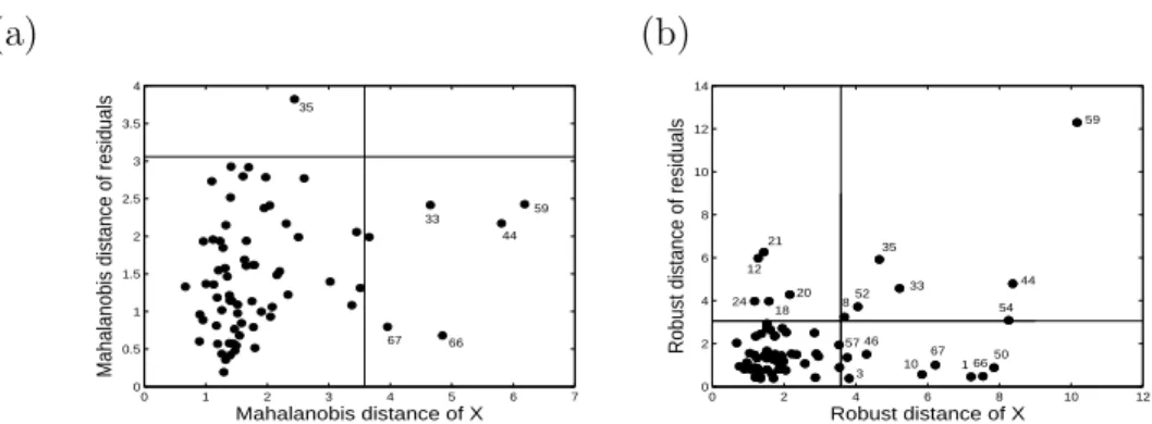
The diagnostic plots in Figure 2 show the Mahalanobis distances of the resid-uals versus the Mahalanobis distances of the explanatory variables (see also Rousseeuw et al. 2004). The left panel presents this plot for the least squares estimator, the right panel for the multivariate GS. For the diagnostic plot based on the robust GS, the Mahalanobis distances are computed using the
robust GS-estimator of Σ, and are therefore called robust distances. The
hor-izontal and vertical lines correspond respectively toqχ2
q,.975 and
q
χ2
p,.975, and
enable us to classify data points into regular observations, vertical outliers, good and bad leverage points. The least squares estimator detects one small vertical outlier and 5 small to moderate good leverage points. On the other hand, the GS-estimator reveals one very large bad leverage point (59), two moderate to large bad leverage points (35 and 44) and two moderate to large vertical outliers (12 and 21). Moreover, there are at least five good leverage points (10, 67, 1, 66, 50). The least squares estimator is thus clearly attracted by the bad leverage points. Table 4 gives 95% confidence intervals, computed with the fast and robust bootstrap discussed in Section 6, for the slope ma-trix based on S- and GS-estimates. The confidence limits using GS-estimates are in bold whenever this interval is shorter than the corresponding interval based on S-estimates. We see that for almost all parameters the GS-estimates yield more precise confidence intervals. This is without surprise, since GS is in general more efficient than S.
(a) (b) 0 1 2 3 4 5 6 7 0 0.5 1 1.5 2 2.5 3 3.5 4 Mahalanobis distance of X
Mahalanobis distance of residuals
35 67 66 33 44 59 0 2 4 6 8 10 12 0 2 4 6 8 10 12 14 Robust distance of X
Robust distance of residuals
21 12 20 18 24 59 35 44 33 52 8 54 50 66 1 67 10 46 57 3
Fig. 2. Diagnostic plots for the school data; (a) Least squares estimator; (b) 50% breakdown GS-estimator
Table 4
95% confidence limits for the school data based on S- and GS-estimates
S-estimate lower upper GS-estimate lower upper
B11 0.109 -0.064 0.265 0.112 -0.052 0.267 B21 4.441 1.660 6.826 4.542 1.980 6.980 B31 0.056 -0.523 0.571 0.019 -0.562 0.490 B41 -0.637 -1.150 -0.202 -0.632 -1.082 -0.219 B51 -0.128 -0.591 0.107 -0.129 -0.513 0.155 B12 0.057 -0.161 0.228 0.053 -0.158 0.223 B22 4.952 2.374 7.913 5.131 2.444 8.304 B32 0.141 -0.625 0.798 0.094 -0.639 0.746 B42 -0.726 -1.295 -0.261 -0.726 -1.190 -0.282 B52 -0.147 -0.575 0.071 -0.147 -0.522 0.084 B13 -0.021 -0.070 0.027 -0.021 -0.065 0.025 B23 1.573 0.884 2.385 1.602 0.861 2.444 B33 0.270 0.099 0.476 0.258 0.075 0.437 B43 0.013 -0.240 0.232 0.018 -0.211 0.223 B53 0.041 -0.049 0.132 0.039 -0.053 0.126 Forbes data
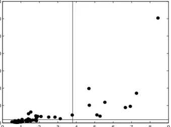
The GS-estimator can also be used as a high-breakdown scatter estimator in
a multivariate location-scale model, takingp= 0 in model (1). Afterwards the
location vector can be estimated using the robust and efficient M-estimator of Lopuha¨a (1992). We illustrate this with a data set taken from the ‘The Data and Story Library’
contains several facts about 79 companies selected from the Forbes 500 list of 1986. We look at the following six variables: Assets (amount of assets in mil-lions), Sales (amount of sales in milmil-lions), Market-value (market-value of the company in millions), Profits (profits in millions), Cash-flow (cash-flow in mil-lions) and Employees (number of employees in thousands). Figure 3 compares the Mahalanobis distances computed with empirical mean and covariance ma-trix (horizontal axis) with the robust distances based on the 50% breakdown GS-estimator (vertical axis) using a distance-distance plot as proposed by Rousseeuw and Van Driessen (1999). If we draw horizontal and vertical lines
at the usual cut off qχ2
6,0.975 = 3.8012, the 9 outliers are detected by both
estimators. However, there are 14 extra observations that have a robust dis-tance above the cutoff while their Mahalanobis disdis-tances lie below the cutoff. Clearly the classical estimates were affected by the presence of these outliers.
0 1 2 3 4 5 6 7 8 9 0 20 40 60 80 100 120 140 Mahalanobis distance of X Robust distance of X
8 Conclusion
In this paper, we discussed generalized S-estimators, i.e. S-estimators applied to the pairwise differences of the observations, in the multivariate regression context. We showed that they maintain the same good properties as in the univariate case, such as a high breakdown point and a higher efficiency than the multivariate regression S-estimators. To compute the GS-estimator, we constructed an algorithm based on improvement steps similar as in the fast S-algorithm for univariate regression. Furthermore we developed a fast and robust bootstrap method for the multivariate GS-estimators to obtain robust inference for the regression slopes. The examples illustrated the robustness and efficiency of the GS-estimator and its corresponding bootstrap inference.
GS-estimators estimate the regression slopes and the residual covariance ma-trix without needing to estimate the intercept. In the special case of the mul-tivariate location-scale model, this implies that we can estimate the scatter matrix without needing to estimate the location of the observations. As illus-trated in the examples, the intercept can easily be estimated afterwards by using the efficient and robust M-estimator of multivariate location of Lopuha¨a (1992), using the residual covariance matrix of the GS-estimator as an initial estimator. In fact, similarly as for MM-estimators (Yohai 1987, Tatsuoka and Tyler 2000) one can also consider to re-estimate the regression slopes using a multivariate regression M-estimator based on an initial GS scatter matrix estimate. However, such an M-step is intended to increase the low efficiency of the initial estimator. Since GS-estimators already have a fairly high efficiency (Table 1), we do not expect that the M-step yields much further improvement.
Finally, let us stress that all the theoretical results obtained in this paper also apply to the multivariate location-scale model, the latter being a special case of the multivariate regression model. The properties of the GS-estimator were not yet investigated in the multivariate location-scale model. The major advantage of the GS-estimators of scatter with respect to most existing robust estimators of scatter is that they have the independency property. Hence, as discussed in the introduction, they are well suited for independent component analysis, and present a high breakdown alternative for the estimators considered by Sirki¨a et al. (2007).
A Appendix
Proof of Theorem 1. Denote by m the number of points in the original
data set of size n that are replaced by arbitrary points. This implies that
the ³n2´ differences in the contaminated data set contain ³m2´+ m(n −m)
contaminated differences. Since we apply the multivariate S-estimator on the set of differences, it follows from Theorem 1 in Van Aelst and Willems (2005) that the maximum number of outliers that is allowed before the estimator breaks down is given by
min(⌈ Ã n 2 ! r⌉,⌈ Ã n 2 ! − Ã n 2 ! r⌉ −hVn)−1
with r = k/supρ and hVn is the maximal number of differences lying on
the same hyperplane. Hence breakdown because the number of contaminated differences exceeds⌈³n2´r⌉ −1, occurs if
à m 2 ! +m(n−m)≥ à n 2 ! r (A.1)
The smallest solution of the corresponding equality−m2+(−1+2n)m−n(n− 1)r = 0 yields m = ⌈n− 1 2 − q 1−4n(1−r) + 4n2(1−r)/2⌉ (which in the limit yields m/n <1−√1−r).
We now consider breakdown because the number of contaminated differences on the same hyperplane exceeds ⌈³n2´−³n2´r⌉ −hVn−1. From condition 1 it
follows that the estimator can break down as soon as
à p+q 2 ! + à m 2 ! +m(p+q)≥ à n 2 ! − à n 2 ! r. (A.2)
The smallest solution of the corresponding equality yields m =⌈1
2 −p−q+
1 2
√
1−4n−4n2r+ 4nr+ 4n2⌉(which in the limit yields m/n <√1−r).
For any C ∈P DS(q), let λ1(C) ≥ λ2(C). . . ≥ λq(C) denote its eigenvalues.
Put
m= min(⌈n−1/2−q1 + (1−r)(4n2−4n)/2⌉,
⌈1/2−p−q+q1 + (1−r)(4n2−4n)/2⌉)−1
We first show thatǫ∗
n> m by showing that the estimator doesn’t break down
if we contaminate at mostm observations. Formally we show that∃M, αonly
depending on Zn, such that for every Zn′ = {(1,(u′i)T,(y′i)T)T; 1 ≤ i ≤ n}
obtained by replacing at most m observations from Zn, we havekBbn(Zn′)k ≤
M and λ1(Σbn(Zn′))≤α and λq(Σbn(Zn′))>0. The norm we use is
kAk= sup
kuk=1k
Auk.
The inequality kABk ≤ kAkkBk holds for any A ∈ Rp×q and B ∈ Rq×r.
Sometimes we will also use the L2-norm kAk2 = (Σi,j|Aij|2)1/2. Since these
norms are topologically equivalent, we know that∃α1, α2 >0 such that ∀B ∈
kwk=kwk2.
Let us denote by Vn the set of the differences corresponding to the data set
Zn, that is, Vn = {((ui −uj)T,(yi −yj)T)T; 1 ≤ i < j ≤ n}. Similarly, Vn′
corresponds to the contaminated data set Z′
n.
W.l.o.g. we assume that c= 1 and thus sup(ρ) = ρ(∞) = 1 such that r =k.
Indeed we can always rescale the functionρif necessary. Sinceρ is continuous
and we have that
à n 2 ! k− à m 2 ! −m(n−m) = à n 2 ! r− à m 2 ! −m(n−m)>0
according to the reverse of (A.1), we can find a smallest radius s > 0 and
cylinder C(0, s2I q) :={(w,v);kvk ≤s} such that X ((ui−uj)T,(yi−yj)T)T∈Vn ρ Ã kyi−yjk s ! = Ã n 2 ! k− Ã m 2 ! −m(n−m).
This yields the determinant V = |s2I
q| = s2q. For the smallest cylinder
C(0, l2I q) = {(w,v);kvk ≤l} such that X ((ui−uj)T,(yi−yj)T)T∈Vn∩Vn′ ρ Ã kyi−yjk l ! = Ã n 2 ! k− Ã m 2 ! −m(n−m) it then holds that|l2I
q|=l2q ≤V. Moreover, X ((u′ i−u ′ j)T,(y ′ i−y ′ j)T)T∈V ′ n ρ Ã kyi′−y′jk l ! ≤ X ((ui−uj)T,(yi−yj)T)T∈Vn∩Vn′ ρ Ã kyi−yjk l ! + Ã m 2 ! +m(n−m) = Ã n 2 ! k.
It follows that for the optimal solutionC(Bbn(Zn′),Σbn(Zn′)) =C(Bbn(Vn′),Σbn(Vn′)) :=
{(w,v); (v−Bbn(Vn′)Tw)TΣbn(Vn′)−1(v−Bbn(Vn′)Tw)≤1} that satisfies X ((u′ i−u ′ j)T,(y ′ i−y ′ j)T)T∈Vn′ ρ³d′ij(Bbn(Vn′),Σbn(Vn′)) ´ ≤ Ã n 2 ! k (A.3)
where d′
ij(Bbn(Vn′),Σbn(Vn′)) = ((r′ij)TΣbn(Vn′)−1r′ij)1/2 with r′ij = y′i − y′j −
b
Bn(Vn′)T(u′i−u′j), we must have that|Σbn(Vn′)| ≤V.
Condition (A.3) implies that the cylinderC(Bbn(Vn′),Σbn(Vn′)) contains a
subcol-lection of at least³n2´−³n2´r points ofV′
n. From the reverse of (A.2) it follows
that this subcollection contains at least ³n2´−³n2´r−³m2´>³p+2q´+m(p+q)
differences that involve at least one original data point ofZn. This inequality
implies one of the two following cases:
• this cylinder contains at leastp+q+ 1 differences between two original data
points not all lying on the same hyperplane.
• the cylinder contains at most ³p+2q´ differences of original data points and
these differences are lying on a hyperplane. The above inequality then im-plies that there is at least 1 contaminated point for which the differences
with p+q+ 1 original data points are lying in the cylinder.
We now show that, for every V > 0, there exists a constant M > 0, only
depending on Zn, such that kBbn(Vn′)k > M implies that the determinant of
b
Σn(Vn′) is larger than V.
Let λ1 ≥. . .≥ λq be the eigenvalues of Σbn(Vn′), then |Σbn(Vn′)|= λ1. . . λq. In
the first case there exists a constantβ >0 such thatλj > βfor allj = 1, . . . , q.
(For everyw∈Rp, the axes of the ellipsoid {v|(v−Bbn(V′
n)Tw)TΣbn(Vn′)−1(v−
b
Bn(Vn′)Tw)≤1} have lengths
q
λj;j = 1, . . . , q.)
For symmetric q×q matrices A, it holds thatλq(A) = infv v
TAv
vTv from which we
obtain that for (w,v)∈ C(Bbn(Vn′),Σbn(Vn′))
In particular, forv=0 we have kBbn(Vn′)Twk2 ≤λ1.
Since C(Bbn(Vn′),Σbn(Vn′)) contains p +q + 1 differences of 2 original points
that are in general position, there exists a constant d > 0, not depending on
b
Bn(Vn′) orΣbn(Vn′), such thatkwk< dimplies that (w,0)∈ C(Bbn(Vn′),Σbn(Vn′)).
If follows that sup kwk=dk
b
Bn(Vn′)Twk2 ≤λ1, so kBbn(Vn′)Tk2 ≤ λd12.
Now consider case 2 where we have at least 1 contaminated point whose differ-ences withp+q+1 original points belongs toC(Bbn(Vn′),Σbn(Vn′)). From the
tri-angle inequality if follows that the³p+q2+1´differences of thesep+q+1 original points belong toC2(Bbn(Vn′),Σbn(Vn′)) ={(w,v); (v−Bbn(Vn′)Tw)TΣbn(Vn′)−1(v− b Bn(Vn′)Tw) ≤ 4}. Because C2(Bbn(Vn′),Σbn(Vn′)) contains ³p+q+1 2 ´ differences of original points which are in general position, then similarly as in case 1 it fol-lows that there exists constants β >0 and d >0 such that kBbn(Vn′)Tk2 ≤ λd12.
Hence, in both cases we obtain that
kBbn(Vn′)k ≤ 1 α1k b Bn(Vn′)k2 = 1 α1k b Bn(Vn′)Tk2 ≤ α2 α1k b Bn(Vn′)Tk ≤ α2√λ1 α1d . Define M = α2V 1/2 α1dβ q−1 2 .
Then we have that kBbn(Vn′)k> M implies that|Σbn(Vn′)|=λ1· · ·λq> V.
As shown,kBbn(Vn′)k> M implies that|Σbn(Vn′)|> V which yields a
contradic-tion. We have thus shown thatkBbn(Vn′)k ≤M. Moreover, since |Σbn(Vn′)| ≤V
and λj > β for allj = 1, . . . , q, there exists a constant 0< α <∞(depending
onβ and V) such that λ1(Σbn(Vn′))≤α.
We now prove thatǫn(Bbn(Vn′)), ǫn(Σbn(Vn′))≤ 1n⌈n−1/2−
q
1 + (1−r)(4n2−4n)/2⌉.
Replace⌈n−1/2−q1 + (1−r)(4n2 −4n)/2⌉points ofZ
V′
n has at least
³n
2
´
r contaminated differences, call this amountm′. Let
C(B, C) ={(w,v); (v−BTw)TC−1(v−BTw)≤1} (A.4)
be a cylinder that satisfies
X ((u′ i−u ′ j)T,(y ′ i−y ′ j)T)T∈V ′ n ρ(d′ij(B, C))≤ Ã n 2 ! k = Ã n 2 ! r. (A.5)
Now suppose that all differences where at least one contaminated point is
involved, are outsideC(B, C). Then
X ((u′ i−u ′ j)T,(y ′ i−y ′ j)T)T∈Vn′ ρ(d′ij(B, C)) = X ((u′ i−u ′ j)T,(y ′ i−y ′ j)T)T∈Vn∩Vn′ ρ(d′ij(B, C))+m′ ≥ Ã n 2 ! r. If m′ = ³n 2 ´ r then ³n2´−m′ = ³n 2 ´ −³n2 ´
r ≥ ³p+q2+1´, so there exists at least one difference ((u′i −u′j)T,(y′
i −yj′)T)T ∈ Vn∩ Vn′ for which d′ij(B, C) > 0.
Because ρ is strictly increasing, this implies that PV′
nρ(d ′ ij(B, C)) > ³n 2 ´ r so we have a contradiction. Hence, any cylinder of type (A.4) that satisfies (A.5)
contains at least one difference involving an outlier. By letting kyk → ∞ for
the contaminated points and also making sure that the distance between them
is large, we have ky1−y2k → ∞ in all cases, hence we can make sure that at
least one of the eigenvalues of C goes to infinity. Therefore, bothBbn(Zn) and
b
Σn(Zn) break down in this case.
We now show that ǫ∗
n≤ (⌈1/2−p−q+
q
1 + (1−r)(4n2−4n)/2⌉)/n.
Con-dition 1 implies that there are at most p+ q original points on the same
hyperplane ofRp+q. Hence, ∃α∈Rq, γ ∈Rp such thatαTyi−γTui = 0 for all i ∈ I ⊂ {1, . . . , n} with size(I) = p+q. If α 6= 0 then ∃B ∈ Rp×q such that
γ =Bα which implies αT(y
i−BTui) = 0,∀i∈I, so yi−BTui ∈S with S a
{DTu;u∈Rp} ⊂S (such aDalways exists). Now replacem=⌈1/2−p−q+
q
1 + (1−r)(4n2−4n)/2⌉observations ofZ
n, not lying onSby ((lu0)T,((B+
tD)Tlu
0)T)T, l = 1, . . . , m for some arbitrarily chosen u0 ∈Rp and t∈R. For
the contaminated points it then holds that the residualsrl(B+tD) equal0and
thus also the differences between residuals of two contaminated data points
equal 0. For the difference of two observations with indices i, j ∈ I we have
that (ri−rj)(B+tD) =yi−yj−BT(ui−uj)−tDT(ui−uj)∈Sand for the
dif-ference of an observation with indexi∈I and a contaminated observation we
have (ri−rl)(B+tD) = ri(B+tD)∈S. Denote{e1, . . . ,eq−1}an orthonormal
basis of S and eq a normed vector orthogonal to S. Denote P = [e1, . . . ,eq].
Consider C of the form C =PΛPT with Λ = diag(λ
1, . . . , λq). Then we have
that ((rl −rl′)(B +tD))TC−1(rl −rl′)(B +tD) = 0 for the difference of 2
outliers. For the observations satisfying (ri −rj)(B +tD) ∈ S, there exists
coefficients ζ1, . . . , ζq such that (ri−rj)(B +tD) =Pqk−=11ζkek. Therefore
((ri−rj)(B+tD))TC−1(ri−rj)(B+tD) = q−1 X k=1 ζkeTk ÃXq l=1 λ−l 1eleTl !qX−1 k=1 ζkek = qX−1 k=1 ζkλ−k1eTk q−1 X k=1 ζkek = q−1 X k=1 ζk2λ−k1. Now Pi<jρ((((ri−rj)(B +tD))TC−1(ri−rj)(B+tD))1/2) = X diff of 2 outliers + X number onS + X remainder ≤ X number onS + Ã n 2 ! r. where number onS =³p+2q´+⌈1/2−p−q+q1 + (1−r)(4n2−4n)/2⌉(p+q). Hence we need X number onS ≤0. (A.6)
By lettingλ1, . . . , λq−1 → ∞we can make ((ri−rj)(B+tD))TC−1(ri−rj)(B+
(Bbn(Zn′),Σbn(Zn′)) satisfies|Σbn(Zn′)| ≤ |C|for any (B+tD, C) satisfying (A.6).
Now |C|=λ1· · ·λq and condition (A.6) does not depend on λq so we can let
λq →0 yielding|C| →0. By lettingt → ∞, we thus obtain that bothBbn(Zn′)
and Σbn(Zn′) break down.
Ifα =0, then γTu
i = 0 for all i∈I. We now put the
m=⌈1/2−p−q+q1 + (1−r)(4n2−4n)/2⌉ outliers on the vertical
hyper-plane γTu
i = 0 at infinity such that at least
³n
2
´ −³n2
´
r differences are lying
on the vertical hyperplane. It can easily be seen that if at least ³n2´−³n2´r points lie on a hyperplane, then this hyperplane is an optimal solution with an accompanying covariance matrix having zero determinant. In this case
how-ever, the hyperplaneγT(u
i−uj) = 0 is vertical such that kBbn(Zn′)k=∞and
|Σbn(Zn′|= 0. ¤
Proof of Theorem 2. Due to equivariance we may assume that B = 0 and
Σ = Iq, so y1 −y2 =ǫ1 −ǫ2 ∼ F. It now suffices to show that BGS(H) = 0.
Since the constant k can be chosen such that k = EF[ρ(kǫ1 −ǫ2k)] which
assures consistency at the model with F the distribution of the difference of
the errors, it follows that ΣGS(H) = Iq. Because BGS is the GS-solution it
satisfies the first order condition:
Z Z
u(dH(r1−r2))(u1−u2)(y1−y2− BGST (H)(u1−u2)) TdH(u
1−u2,y1−y2) = 0 (A.7)
Now suppose that BGS 6= 0. Let λ1, . . . , λq be the eigenvalues of ΣGS and
v1, . . . ,vqthe corresponding eigenvectors. There will be at least one 1≤j ≤q
such that BGSvj 6= 0. Fix thisj. From (A.7) it follows that we should have
ZZ
vTj(BGST (u1−u2))u(dH(r1−r2))(y1−y2− BTGS(H)(u1−u2))TvjdF(y1−y2)dG(u1−u2) = 0
Z Rpv T j(BTGS(u1−u2))I(u1−u2)dG(u1−u2) = 0 (A.8) with I(u1−u2) = Z Rqu(dH(r1−r2))(y1−y2− B T GS(H)(u1−u2))TvjdF(y1−y2).
Fix u1 −u2 and set d = (d1, . . . , dq)T := BTGS(u1 − u2). Since y1 − y2 is
spherically symmetrically distributed, for computingI(u1−u2) we may assume
w.l.o.g. that ΣGS = diag(λ1. . . , λq) as well asvj = (1,0, . . . ,0)T.
Becauseu(s) =ρ′(s)/sonly differs from zero ifs ≤c. Withs=dH(r1−r2) we
obtain r Pq j=1 (y1j−y2j−dj)2 λj ≤c. For every d1−c √ λ1 ≤ y11−y21≤ d1+c √ λ1 denote C(y11−y21) = (y12−y22, . . . , y1q−y2q)∈R q−1 | q X j=2 (y1j−y2j −dj)2 λj ≤ c2−(y11−y21−d1) 2 λ1
Then we can rewriteI(u1 −u2) as
I(u1−u2) = Z d1+c√λ1 d1−c√λ1 Z C(y11−y21) u(dH(r1−r2))(y11−y21−d1)g((y11−y21)2+· · ·+ (y1q−y2q)2)d(y11−y21). . . d(y1q−y2q) = Z c√λ1 −c√λ1 t Z C(d1+t) u(dH(r1−r2))g((d1+t)2+· · ·+ (y1q−y2q)2)d(y12−y22). . . d(y1q−y2q)dt.
Since C(d1+t) = C(d1−t) it follows that
I(u1−u2) = Z c√λ1 0 t Z C(d1+t) u(dH(r1−r2))g ³ (d1+t)2+ (y12−y22)2 +· · ·+ (y1q−y2q)2 ´ −g³(d1−t)2+ (y12−y22)2+· · ·+ (y1q−y2q)2 ´ d(y12−y22). . . d(y1q−y2q)dt. If d1 > 0 we have (d1 +t)2 + (y12 −y22)2 +· · ·+ (y1q −y2q)2 > (d1 −t)2 +
(y12−y22)2+· · ·+ (y1q −y2q)2 (for t > 0) and since g is strictly decreasing
I(u1−u2)>0 and that d1 = 0 yields I(u1−u2) = 0. Hence, we have shown
thatvTj(BT
GS(u1−u2))>0 impliesI(u1−u2)<0 and ifvjT(BGST (u1−u2))<0,
then I(u1 −u2) > 0. Also vTj(BGST (u1 −u2)) = 0 implies I(u1 −u2) = 0.
However, due to the regularity condition 3 on the model distribution, the
latter event occurs with probability less than 1−r. Therefore, we obtain
Z
Rpv
T
j(BTGS(u1−u2))I(u1−u2)dG(u1−u2)<0
which contradicts (A.8), so we conclude thatBGS = 0. ¤
Proof of Theorem 3. It can be shown that the GS-functional GS(H) =
(BGS(H),ΣGS(H)) can be represented (as in Lopuha¨a 1989) by the following
equations ZZ u(dH(r1−r2))(u1−u2)(y1−y2− BTGS(H)(u1 −u2))TdHdH = 0 (A.9) ZZ qu(dH(r1−r2))(y1−y2− BGST (H)(u1−u2))(y1−y2− BGST (H)(u1−u2))TdHdH = ZZ v(dH(r1−r2))dHdHΣGS(H) (A.10)
with (u1,y1) and (u2,y2) realizations of two independent variables∼H. ri =
yi− BTui −α so r1 −r2 = y1 −y2 − BTGS(H)(u1 −u2) and dH(r1 −r2) =
((r1−r2)TΣ−GS1(H)(r1−r2))1/2.
We first derive the influence function of the slope matrixBGSatH0. From (A.9)
it follows that ∂ ∂ǫ ZZ u(dHǫ(r1−r2))(u1−u2)(y1−y2− B T GS(Hǫ)(u1−u2))TdHǫdHǫ|ǫ=0 = 0
∂ ∂ǫ · (1−ǫ)2 ZZ u(dHǫ(r1−r2))(u1−u2)(y1−y2− B T GS(Hǫ)(u1−u2))TdH0dH0 + 2ǫ(1−ǫ) ZZ u(dHǫ(r1 −r2))(u1−u2)(y1−y2− B T GS(Hǫ)(u1−u2))TdH0∆z0 +ǫ2 ZZ u(dHǫ(r1−r2))(u1−u2)(y1−y2 − B T GS(Hǫ)(u1 −u2))T∆2z0 ¸ |ǫ=0 = 0
Differentiating with respect toǫ and accounting for equation (A.9) yields
∂ ∂ǫ ·ZZ u(dHǫ(r1−r2))(u1−u2)(y1−y2− B T GS(Hǫ)(u1−u2))TdH0dH0 ¸ |ǫ=0 + 2 ZZ u(dH0(r1−r2))(u1−u2)(y1−y2− B T GS(H0)(u1−u2))TdH0∆z0 = 0
Rewriting term 1, we get
− ZZ u′(dH0(r1 −r2)) ∂ ∂ǫdHǫ(r1−r2)|ǫ=0(u1 −u2)(y1−y2− B T GS(H0)(u1−u2))TdH0dH0 − ZZ u(dH0(r1−r2))(u1−u2)(u1 −u2) T(−IF(z 0;BGS, H0))dH0dH0 = 2 Z u(dH0(r1−r0))(u1−u0)(y1 −y0− B T GS(H0)(u1−u0))TdH0
SinceBGS(H0) = 0 and ΣGS(H0) =Iqwe havedH0(r1−r2) =
q (y1−y2)T(y1−y2) = ky1−y2k. Hence, we obtain − ZZ u′(ky1 −y2k) ∂ ∂ǫdHǫ(r1−r2)|ǫ=0(u1−u2)(y1−y2) TdH 0dH0 + ZZ u(ky1−y2k)(u1−u2)(u1−u2)TdH0dH0IF(z0;BGS, H0) = 2 Z u(dH0(r1−r0))(u1−u0)(y1 −y0) TdH 0 (A.11) Using that ∂ ∂ǫdHǫ(r1−r2)|ǫ=0 =(−IF(z0;BGS, H0) T(u 1−u2))T ky1−y2k (y1−y2) + 1 2 (y1−y2)T ky1−y2k IF(z0; Σ−GS1, H0)(y1−y2)
− ZZ u′(ky1−y2k) ∂ ∂ǫdHǫ(r1−r2)|ǫ=0(u1−u2)(y1−y2) TdH 0dH0 = ZZ (u1−u2)(u1−u2)TdGdGIF(z0;BGS, H0) ZZ u′ (ky1−y2k) ky1−y2k (y1−y2)(y1−y2)TdF0dF0 −12 ZZ (u1−u2)dGdG ZZ u′ (ky1−y2k) ky1−y2k (y1−y2)TIF(z0; Σ−GS1, H0)(y1−y2)(y1−y2)TdF0dF0
The last term vanishes because EG×G[u1 −u2] = 0. Hence equation (A.11)
becomes: EG×G[(u1−u2)(u1−u2)T]IF(z0;BGS, H0) ·ZZ u′( ky1−y2k) ky1−y2k (y1−y2)(y1−y2)TdF0dF0 + ZZ u(ky1−y2k)dF0dF0 ¸ = 2 Z u(dH0(r1−r0))(u1−u0)(y1−y0) TdH 0
From symmetry it follows that RR u′(ky1−y2k)
ky1−y2k (y1 − y2)(y1 − y2) TdF 0dF0 = RR u′(ky 1 −y2k)1qky1−y2kdF0dF0Iq hence we obtain IF(z0;BGS, H0) =EG×G[(u1−u2)(u1−u2)T]−1 2R u(ky1−y0k)(u1−u0)(y1−y0)TdH0 EF0×F0 h u′(ky1−y2k)ky1−y2k q +u(ky1−y2k) i Usingu′(t)t =ψ′(t)−ψ(t)/t yields IF(z0;BGS, H0) =EG×G[(u1−u2)(u1−u2)T]−1 2R(u1−u0)dGR u(ky1−y0k)(y1−y0)TdF0 EF0×F0 h 1 qψ′(ky1−y2k) + ³ 1−1 q ´ u(ky1−y2k) i = [Cov(u)]−1 R (u1−u0)dGR u(ky1−y0k)(y1 −y0)TdF0 EF0×F0 h 1 qψ′(ky1−y2k) + ³ 1− 1 q ´ u(ky1−y2k)i
The influence function of ΣGSis derived in a similar way, now by differentiating
equation (A.10) ∂ ∂ǫ Z Z qu(dHǫ(r1−r2))(y1−y2− B T GS(Hǫ)(u1−u2))(y1−y2− BGST (Hǫ)(u1−u2))TdHǫdHǫ|ǫ=0 = ∂ ∂ǫ Z Z v(dHǫ(r1−r2))dHǫdHǫ|ǫ=0ΣGS(H0) + Z Z v(dH0(r1−r2))dH0dH0IF(z0; ΣGS, H0)
Differentiating and taking (A.10) into account leads to EH0×H0[v(ky1−y2k)]IF(z0,ΣGS, H0) +1 2 ZZ v′(ky 1−y2k) ky1−y2k (y1−y2)TIF(z0,ΣGS−1, H0)(y1−y2)dH0dH0Iq −q2 ZZ u′(ky 1−y2k) ky1−y2k (y1 −y2)TIF(z0,Σ−GS1, H0)(y1−y2)(y1−y2)(y1−y2)TdH0dH0 = 2 Z qu(ky1−y0k)(y1−y0)(y1−y0)TdH0−2 Z v(ky1−y0k)dH0Iq
and we rewrite this as (using IF(z0; Σ−GS1, H0) =−IF(z0; ΣGS, H0))
EH0×H0[v(ky1−y2k)]IF(z0,ΣGS, H0) −12 q X i,j=1 ZZ v′ (ky1−y2k) ky1−y2k (y1−y2)Ti IF(z0,(ΣGS)ij, H0)(y1−y2)jdH0dH0Iq +q 2 q X i,j=1 ZZ u′( ky1−y2k) ky1−y2k (y1−y2)iIF(z0,(ΣGS)ij, H0)(y1−y2)j(y1−y2)(y1−y2)TdH0dH0 = 2 Z qu(ky1−y0k)(y1−y0)(y1−y0)TdH0−2 Z v(ky1−y0k)dH0Iq
Eliminating the terms which are 0 and following Lopuha¨a (1999, Lemma 2.1) it holds that γ1IF(z0; ΣGS, H0)−γ2trIF(z0; ΣGS, H0)Iq = 2 Z qu(ky1−y0k)(y1−y0)(y1−y0)TdH0 −2 Z v(ky1−y0k)dH0Iq where γ1=EF0×F0[v(ky1 −y2k)] + 1 q+ 2EF0×F0 h u′(ky1−y2k)(ky1−y2k)3 i γ2=EF0×F0 " 1 2qv ′(ky 1−y2k)ky1 −y2k # − 2(q1+ 2)EF0×F0 h u′(ky1 −y2)ky1−y2k3 i