Research Online
Research Online
Centre for Statistical & Survey Methodology
Working Paper Series Faculty of Engineering and Information Sciences
2009
Asymptotics for General Multivariate Kernel Density Derivative Estimators
Asymptotics for General Multivariate Kernel Density Derivative Estimators
J. E. Chacon
Universidad de Extremadura, Spain
T. Duon
Institut Pasteur, France
M. P. Wand
University of Wollongong, [email protected]
Follow this and additional works at: https://ro.uow.edu.au/cssmwp Recommended Citation
Recommended Citation
Chacon, J. E.; Duon, T.; and Wand, M. P., Asymptotics for General Multivariate Kernel Density Derivative Estimators, Centre for Statistical and Survey Methodology, University of Wollongong, Working Paper 08-09, 2009, 30p.
https://ro.uow.edu.au/cssmwp/28
Research Online is the open access institutional repository for the University of Wollongong. For further information contact the UOW Library: [email protected]
Copyright © 2008 by the Centre for Statistical & Survey Methodology, UOW. Work in progress, no part of this paper may be reproduced without permission from the Centre.
Centre for Statistical & Survey Methodology, University of Wollongong, Wollongong NSW 2522. Phone +61 2 4221 5435, Fax +61 2 4221 4845. Email: [email protected]
Centre for Statistical and Survey Methodology
The University of Wollongong
Working Paper
08-09
Asymptotics for General Multivariate Kernel Density Derivative
Estimators.
estimators
Jos´e E. Chac´on∗, Tarn Duong† and M. P. Wand‡ May 28, 2009
Abstract
We investigate general kernel density derivative estimators, that is, kernel estimators of multivariate density derivative functions using general (or unconstrained) bandwidth matrix selectors. These density derivative estimators have been relatively less well re-searched than their density estimator analogues. A major obstacle for progress has been the intractability of the matrix analysis when treating higher order multivariate derivatives. With an alternative vectorization of these higher order derivatives, these mathematical intractabilities are surmounted in an elegant and unified framework. The finite sample and asymptotic analysis of squared errors for density estimators are gen-eralized to density derivative estimators. Moreover, we are able to exhibit a closed form expression for a normal scale bandwidth matrix for density derivative estimators. These normal scale bandwidths are employed in a numerical study to demonstrate the gain in performance of unconstrained selectors over their constrained counterparts.
Keywords: asymptotic mean integrated squared error, normal scale rule, optimal, uncon-strained bandwidth matrices.
∗
Departamento de Matem´aticas, Universidad de Extremadura, Spain. E-mail: [email protected]
†
Institut Pasteur, Groupe Imagerie et Mod´elisation; CNRS, URA 2582, F-75015, Paris, France. Email:
‡
School of Mathematics and Applied Statistics, University of Wollongong, Wollongong, Australia. E-mail: [email protected]
1
Introduction
Estimating probability density functions with kernel functions has had notable success due to their ease of interpretation and visualization. On the other hand, estimating derivatives of density functions has received less attention. This is partially because it is a more chal-lenging theoretical problem (especially for multivariate data). Nonetheless there remains much information about the structure of a density function which is not easily ascertained from the density function itself. For example, the local maxima and minima are where there are zero first derivatives and non-zero second derivatives. One of the original papers on ker-nel density estimation (Parzen, 1962) was also concerned with the estimating the global mode of the density function, though not from a density derivative point of view. We can recast this problem as a density derivative estimation problem: find the local maxima via derivative estimates and the global mode follows as the largest of these local maxima. The focus on a mode as a single point can be extended to the region immediately surrounding the mode, known as a bump or modal region. Modal regions can be used to determine the existence of multi-modality and/or clusters. Godtliebsen, Marron and Chaudhuri (2002)’s feature significance technique for bump-hunting relies on estimating and characterizing the first and second derivatives for bivariate data. In an econometrics setting, the Engel curve describes the demand for a good/service as a function of income. It classifies goods/services based on the slope of their Engel curve so the first derivative is an essential component for interpreting these curves, see Hildenbrand and Hildenbrand (1986). In a more general setting, Singh (1977) suggests as an application of the multivariate density derivatives to estimate the Fisher information matrix in its translation parameter form.
The first paper to be concerned with univariate kernel density derivative estimation ap-pears to be Bhattacharya (1967), followed by Schuster (1969) and Singh (1979, 1987). Singh (1976) studies a multivariate estimator with a diagonal bandwidth matrix, and H¨ardle, Marron and Wand (1990) with the bandwidth parametrized as a constant times the iden-tity matrix. This previous research has mostly focused on constrained parametrizations of the bandwidth matrix since they simplify the matrix analysis compared to the gen-eral, unconstrained parametrization. Analyzing squared error measures for general kernel density derivative estimators has reached an impasse using the traditional vectorization of higher order derivatives of multivariate functions (a vectorization transforms the higher order derivative tensor into a more tractable vector form). To tackle this problem, we intro-duce an alternative vectorization of higher order derivatives. This vectorization is a subtle rearrangement of the traditional vectorization which allows us to write down with the same ease all the usual error expressions from the density estimation case. Thus we generalize the usual squared error analysis for kernel density derivative estimators. Furthermore, we are able to write down a closed form expression for a normal scale bandwidth matrix, i.e., the optimal bandwidth for therth order derivative of a normal density with normal kernels.
Normal scale selectors were the first step which eventually lead to the development of the now widely used bandwidth selectors for density estimation: we set up a similar starting point for future bandwidth selection in density derivative estimation.
In Section 2 we define a kernel estimator of a multivariate density derivative, and provide the results for mean integrated square convergence both asymptotically and for finite sam-ples. The influence of the bandwidth matrix on convergence is established here. In Section 3 we focus on the class of normal mixture densities. Estimation of these densities with normal kernels produces further simplified special cases of the results in the Section 2, where we de-velop a normal scale bandwidth selector. In Section 4, we use these normal scale selectors to quantify the improvement in asymptotic performance when using unconstrained matrices. We illustrate the normal scale selectors on data arising from high throughput biotechnology in Section 5. The usual normal scale selectors based on the density function may lead to insufficient smoothing when estimating the density curvature (or second derivative). We conclude with a discussion in Section 6.
2
Kernel density derivative estimation
The current state of multivariate kernel density estimation has reached maturity, and recent advances there can be carried over to the density derivative case. To proceed, we use the linearity of the kernel density estimator to define a kernel density derivative estimator. The usual performance measure for kernel density estimation is the mean integrated squared error (MISE) which is easily extended to cover density derivatives.
We introduce some notation needed to state our problem. For a matrixA we denote
A⊗r= r O i=1 A= rmatrices z }| { A⊗ · · · ⊗A
the rth Kronecker power of A. If A ∈ Mm×n (i.e., A is a matrix of order m×n) then
A⊗r∈ Mmr×nr, therefore, we will adopt the convention A⊗1 =A andA⊗0= 1∈R.
Iff:Rd→Ris a real function of a vector variable we denoteD⊗rf(x)∈Rd
r
the vector containing all the partial derivatives of orderr off atx, arranged so that we can formally write
D⊗rf = ∂f (∂x)⊗r.
Thus we write therth derivative off as a vector of length dr, and not as an r-fold tensor array or as a matrix. Moreover, if f:Rd → Rp is a vector function of a vector variable,
with componentsf = (f1, . . . , fp) then we defineD⊗rf(x)∈Rpd
r to be D⊗rf(x) = D⊗rf1(x) .. . D⊗rfp(x) .
Notice that, using this notation, we have D(D⊗rf) = D⊗(r+1)f. Also, the gradient of f
is just D⊗1f and the Hessian Hf = ∂2f /(∂x∂xT) is such that vecHf =D⊗2f, where vec denotes the vector operator (see Henderson and Searle (1979)). This vectorization carries some redundancy, for example, D⊗2f contains repeated mixed partial derivatives whereas the usual vectorization vechHf contains only the unique second order partial derivatives, with vech denoting the vector half operator (see Henderson and Searle (1979)). The latter is usually preferred since it is minimal and its matrix analysis is not more complicated than the former. However for r > 2, it appears that the matrix analysis using a generalization of the vector half operator becomes intractable. Other authors have used the same vec-torization we propose to develop results for higher order derivatives: Holmquist (1996a) computes derivatives of the multivariate normal density function and Chac´on and Duong (2008) compute kernel estimators of multivariate integrated density derivative functionals. Suppose now that f:Rd →R is a density and we want to estimate D⊗rf(x) for some
r∈N. To this end, we use the kernel estimator \D⊗rf(x;H) =D⊗rfˆ(x;H), where given a
random sampleX1,X2, . . . ,Xd drawn fromf,
ˆ f(x;H) =n−1 n X i=1 KH(x−Xi) (1)
denotes the multivariate kernel density estimator with kernelK and bandwidth matrixH, withKH(x) =|H|−1/2K(H−1/2x). The conditions onK and Hwill be given later. Notice
that alternative expressions for\D⊗rf(x;H) are
\ D⊗rf(x;H) =n−1 n X i=1 D⊗rKH(x−Xi) (2) =n−1(H−1/2)⊗r n X i=1 (D⊗rK)H(x−Xi) =n−1|H|−1/2(H−1/2)⊗r n X i=1 D⊗rK H−1/2(x−Xi) .
The last expression in the previous display is quite helpful for implementing the estimator, because it separates the roles of K and H. This is the multivariate generalization of the kernel estimator which appears, for instance, in H¨ardle, Marron and Wand (1990) and Jones (1994).
Here, the most general (unconstrained) form of the bandwidth matrix is used. In contrast, earlier papers considered this type of kernel estimator, but with constrained parametrizations of the bandwidth matrix, e.g. H¨ardle, Marron and Wand (1990) used a parametrization whereH ish2 multiplied by the identity matrix, and Singh (1976) used H = diag(h21, h22, . . . , h2d). However, in the case r = 0 (estimation of the density itself), Wand and Jones (1993) provide examples that show that a significant gain may be achieved
by using unconstrained parametrizations over constrained ones; see also Chac´on (2009). We generalize these results to arbitrary derivatives in Section 4.
We measure the error of the kernel density derivative estimator at the pointxby using the mean squared error (MSE), defined as
MSE(x;H)≡MSE{\D⊗rf(x;H)}=Ek\D⊗rf(x;H)−D⊗rf(x)k2,
withk · k standing for the Euclidean norm; that is, kvk2 =vTv = tr(vvT) for a vector v,
where trA is short for the trace of a matrix A. We have the two forms MSE(x;H) and MSE{\D⊗rf(x;H)}, depending on whether we wish to suppress the explicit dependence on
\
D⊗rf or not. It is easy to check that we can split MSE(x;H) = B2(x;H) + V(x;H), where
B2(x;H) =kE\D⊗rf(x;H)−D⊗rf(x)k2
V(x;H) =Ek\D⊗rf(x;H)−E\D⊗rf(x;H)k2
Analogously, as a global measure of the performance of the estimator we will use the mean integrated squared error, defined as
MISE(H)≡MISE{\D⊗rf(·;H)}= Z
MSE{\D⊗rf(x;H)}dx.
All the results in this paper rely on the following assumptions on the bandwidth matrix, the density function and the kernel function:
(A1) His a bandwidth matrix which is a symmetric and positive-definite matrix, and such that every element ofH→0 and n−1|H|−1/2(H−1)⊗r→0 as n→ ∞.
(A2) f is a density function for which all partial derivatives up to order (r+ 2) inclusive exist, all its partial derivatives of order r are square integrable, and all its partial derivatives of order (r+ 2) are bounded, continuous and square integrable.
(A3) K is a kernel which is a positive, symmetric, square integrable density function such that R xxTK(x)dx = m2(K)Id for some real number m2(K) and Id is the identity
matrix of orderd, and all its partial derivatives of orderr are square integrable. This is not the minimal set of assumptions but it provides a useful starting point for quan-tifying the following squared error results. We leave it to future research to reduce these assumptions.
For any vector function g:Rd→Rp denote
R(g) =
Z
g(x)g(x)Tdx∈ Mp×p.
Also, for an arbitrary kernelLwe write
RL,H,r(f) =
Z
where the convolution operator is applied to each component of D⊗rf(x) separately. Ex-panding all the terms in the bias-variance decomposition we obtain the following exact representation of the MISE function.
Theorem 1. Assume that (A1)–(A3) hold. The MISE function can be expressed as
MISE{\D⊗rf(·;H)}= trR(D⊗rf) +n−1|H|−1/2tr (H−1)⊗rR(D⊗rK)
+ (1−n−1) trRK∗K,H,r(f)−2 trRK,H,r(f).
The proof of this, along with the proofs for all other theorems in this paper, are deferred to the Appendix.
The form of the MISE given in the above theorem involves a complicated dependence on the bandwidth matrixHvia the Rfunctionals. To show this dependence more clearly, we search for a more mathematically tractable form of the MISE. The next result provides an asymptotic representation of the MISE function, and can be viewed as an extension of Formula (4.10) in Wand and Jones (1995, p. 98), which corresponds to the caser= 0.
Theorem 2. Assume that (A1)–(A3) hold. We can expand
MISE{\D⊗rf(·;H)}= AMISE{\D⊗rf(·;H)}+o n−1|H|−1/2trr(H−1) + tr2H , where AMISE{D\⊗rf(·;H)}=n−1|H|−1/2tr (H−1)⊗rR(D⊗rK) +m2(K)2 4 tr (Idr⊗vecT H)R(D⊗(r+2)f)(Idr ⊗vecH).
The AMISE-optimal bandwidth matrixHAMISE is defined to be the matrix, amongst all
symmetric positive definite matrices, which minimizes AMISE{\D⊗rf(·;H)}. Next we give
the order of such a matrix, and the order of the resulting minimal AMISE.
Theorem 3. Assume that (A1)–(A3) hold. Every entry of the optimal bandwidth matrix
HAMISE is of order O(n−2/(d+2r+4)). As a consequence, the minimal achievable AMISE,
minHAMISE{\D⊗rf(·;H)}, is of order O(n−4/(d+2r+4)).
Theorems 1, 2 and 3 generalize the existing MISE, AMISE and HAMISE results for
constrained to unconstrained bandwidth matrices. These rates of convergence reveal the relationship with dimension d and derivative order r. As either of these increase, the minimum achievable of the AMISE increases. Though we note that, at least asymptotically, the marginal increase in difficulty in estimating a derivative an order higher is the same as estimating a density two dimensions higher.
To appreciate the ramifications of these three theorems, we briefly review the litera-ture for kernel density derivative estimation. Bhattacharya (1967) shows that the rate of
convergence in probability of a univariate kernel density derivative estimator with a sec-ond order kernel is bounded byn−1/(2r+4), without developing intermediate squared error convergence results. Schuster (1969) establishes the same rate for a wider class of kernels. Singh (1979, 1987) establish, for his specially constructed univariate kernel estimator, that
n−2(p−r)/(2p+1) is the MSE and MISE rate of convergence respectively. This estimator
em-ploys kernels whoserth moment is 1 and all otherjth moments are zero,j= 0,1, . . . , p−1,
j6=r forp > r. The order of these kernels is greater than or equal to r. Since we assume second order kernels (assumption (A3)), then Theorem 3 will not generalize this result for
r >2. For second order kernels, Wand and Jones (1995, p. 49) show that p=r+ 2 which gives the MISE to beO(n−4/(2r+5)), which is indeed Theorem 3 withd= 1.
Ford-variate density derivative estimation, Stone (1980) states that for any linear non-parametric estimator, the minimum achievable MSE of an estimator ofg, a scalar functional of D⊗rf, is O(n−2(p−r)/(2p+d)) where p > r and the pth order derivative of g is bounded. From assumption (A2), we have thatp=r+ 2 so the MISE rate isO(n−4/(d+2r+4)) which is exactly the same rate as Theorem 3. However this general result is unable to elucidate certain key questions specific to kernel estimators, such as the relationship between the convergence rate and the bandwidth matrix, which Theorems 1, 2 and 3 demonstrate clearly. Singh (1976) shows that a multivariate kernel density derivative estimator with a diagonal bandwidth matrix H = diag(h21, h22, . . . , h2d) is mean square convergent, though he is not able to quantify the rate of convergence. More recently Duong, Cowling, Koch and Wand (2008) establish that the MISE convergence rate for kernel estimators with unconstrained bandwidth matrices, isn−4/(d+6) and n−4/(d+8) for r= 1,2. Theorem 3 extends these two special cases to arbitraryr.
So far we have only considered scalar functionals of the expected value and the variance of\D⊗rf. For completeness, the following theorem gives these quantities in their vector and
matrix form. This theorem is a generalization of the results obtained by Duong, Cowling, Koch and Wand (2008) forr = 1,2 to arbitrary r.
Theorem 4. Assume (A1)–(A3) hold. The expected value of \D⊗rf(x;H) is
E \D⊗rf(x;H) =D⊗rf(x) +12m2(K)(Idr ⊗vecTH)D⊗(r+2)f(x) +O(tr2H)1dr
and the variance is
Var\D⊗rf(x;H) =n−1|H|−1/2(H−1/2)⊗rR(D⊗rK)(H−1/2)⊗rf(x) +o(n−1|H|−1/2trrH−1)J
dr
where the elements of 1p ∈Rp and Jp ∈ Mp×p are all ones.
3
Normal mixture densities
In this section we study in detail the problem in the normal mixture case. We start with a single normal density, whenK =φwith φ the density of the standard d-variate normal
distribution,φ(x) = (2π)−d/2exp(−xTx/2), and whenf =φΣ(· −µ) a normal density with meanµand varianceΣ.
The MISE and AMISE expressions in the normal case are closely related to the moments of quadratic forms in normal variables. Given two symmetric matricesA and B inMd×d,
we will write
µr,s(A,B)≡E[(zTA−1z)r(zTB−1z)s] and µr(A)≡µr,0(A,I)
wherez is ad-variate random vector with standard normal distribution.
Theorem 5. Assume that (A1) holds. Further assume that f is a normal density with
meanµ and varianceΣ; and that K is the normal kernel. The MISE function admits the explicit expression
MISE{\D⊗rf(·;H)}= 2−(d+r)π−d/2
|Σ|−1/2µr(Σ) +n−1|H|−1/2µr(H)
+ (1−n−1)|H+Σ|−1/2µr(H+Σ)−2(d+2r+2)/2|H+ 2Σ|−1/2µr(H+ 2Σ) .
As expected, an explicit form of the minimizer of the MISE is not available.
To rewrite Theorem 5 without the µr functionals, we use Theorem 1 in Holmquist
(1996b) which shows that
µr(A) = OF(2r)(vecT A−1)⊗rSd,2r(vecId)⊗r
where OF(2r) = (2r−1)(2r−3)· · ·5·3·1 denotes the odd factorial andSm,n ∈ Mmn×mn
is the symmetrizer matrix of orderm, n; see Holmquist (1996a,b). These references contain long technical definitions of the symmetrizer matrix, which we do not reproduce here. Instead we focus on the action of the symmetrizer matrix on Kronecker products of vectors. Let xi ∈ Rp, i = 1, . . . n, and X∗ = {x∗1, . . . ,x∗n} be a permutation of {x1, . . .xn}. The
symmetrizer matrix maps the product Nn
i=1xi to a linear combination of products of all
possible permutations ofx1, . . . ,xn Sm,n n O i=1 xi = 1 n! X all X∗ n O i=1 x∗i.
More explicitly for a 3-fold product,Sm,3(x1⊗x2⊗x3) = 16[x1⊗x2⊗x3+x1⊗x3⊗x2+
x2⊗x1⊗x3+x2⊗x3⊗x1+x3⊗x1⊗x2+x3⊗x2⊗x1].
Corollary 1. Under the conditions of Theorem 5, the MISE function admits the explicit
expression
MISE{\D⊗rf(·;H)}= 2−(d+r)π−d/2OF(2r)
|Σ|−1/2(vecT Σ−1)⊗r+|H|−1/2(vecTH−1)⊗r + (1−n−1)|H+Σ|−1/2(vecT(H+Σ)−1)⊗r
This corollary has the advantage of showing the explicit dependence of the MISE on the bandwidth matrix H. However, the direct computation of Sd,2r ∈ Md2r×d2r may be
an onerous task; for example, for d=r = 4, S4,8 is a 65536×65536 matrix. In contrast,
although Theorem 5 does not express the explicit dependence of the MISE on H due to the use of theµr functionals, formula (6) in Holmquist (1996b) gives the computationally efficient recursive expression
µr(A) = (r−1)! 2r−1 r−1 X j=0 tr A−(r−j) j! 2j µj(A). (3)
Here, we understand A−p= (A−1)p forp >0 and, consequently,A0=Id.
An analogous expression of the AMISE is given below. In this case, we can also write down an explicit expression for its minimizer.
Theorem 6. Under the conditions of Theorem 5, the AMISE function admits the explicit
expression
AMISE{\D⊗rf(·;H)}= 2−(d+r)π−d/2
n−1|H|−1/2µr(H) + 161|Σ|−1/2µr,2(Σ,Σ1/2H−1Σ1/2) .
The value of Hthat minimizes this function is
HAMISE = 4 d+ 2r+ 2 2/(d+2r+4) Σn−2/(d+2r+4).
The AMISE expression in Theorem 6 can be rewritten without µr functionals. From
Theorem 5 in Holmquist (1996b),
µr,s(A,B) = OF(2r+ 2s)[(vecT A−1)⊗r⊗(vecT B−1)⊗s]Sd,2r+2s(vecId)⊗(r+s).
Corollary 2. Under the conditions of Theorem 5, the AMISE function admits the explicit
expression
AMISE{D\⊗rf(·;H)}= 2−(d+r)π−d/2
OF(2r)n−1|H|−1/2(vecT H−1)⊗rSd,2r(vecId)⊗r
+161|Σ|−1/2OF(2r+ 4)[(vecTΣ−1)⊗r⊗ {vecT(Σ−1/2HΣ−1/2)}⊗2] ×Sd,2r+4(vecId)⊗(r+2) .
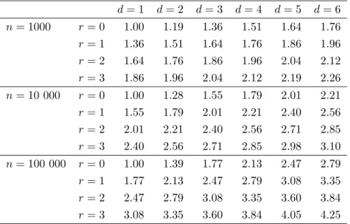
To facilitate the comparison of the extra amount of smoothing induced for higher di-mensions and higher derivatives for standard normal densities, we examine the ratio
hAMISE(d, r, n) hAMISE(1,0, n) = 3 4 1/5 4 d+ 2r+ 2 1/(d+2r+4) n(d+2r−1)/(5d+10r+20)
where HAMISE(d, r, n) = h2AMISE(d, r, n)Id is the AMISE-optimal bandwidth for the
d= 1 d= 2 d= 3 d= 4 d= 5 d= 6 n= 1000 r = 0 1.00 1.19 1.36 1.51 1.64 1.76 r = 1 1.36 1.51 1.64 1.76 1.86 1.96 r = 2 1.64 1.76 1.86 1.96 2.04 2.12 r = 3 1.86 1.96 2.04 2.12 2.19 2.26 n= 10 000 r = 0 1.00 1.28 1.55 1.79 2.01 2.21 r = 1 1.55 1.79 2.01 2.21 2.40 2.56 r = 2 2.01 2.21 2.40 2.56 2.71 2.85 r = 3 2.40 2.56 2.71 2.85 2.98 3.10 n= 100 000 r = 0 1.00 1.39 1.77 2.13 2.47 2.79 r = 1 1.77 2.13 2.47 2.79 3.08 3.35 r = 2 2.47 2.79 3.08 3.35 3.60 3.84 r = 3 3.08 3.35 3.60 3.84 4.05 4.25
Table 1: Comparison of extra smoothing induced for higher dimensions and higher or-der or-derivatives for a standard normal density. Each table entry contains the value of
hAMISE(d, r, n)/hAMISE(1,0, n).
andr = 0,1,2,3. These ratios are the same for different combinations of dand r whenever
d+ 2r are the same.
The normal scale bandwidth selector is obtained by replacing the varianceΣinHAMISE
from Theorem 6 by an estimate ˆΣ
ˆ HNS= 4 d+ 2r+ 2 2/(d+2r+4) ˆ Σn−2/(d+2r+4). (4)
We can use (4) as a starting point to develop consistent data-driven bandwidth matrices. Consistent univariate selectors for density derivatives include the unbiased cross validation selector of H¨ardle, Marron and Wand (1990), and the selector of Wu (1997) and Wu and Lin (2000). The performance of the multivariate versions of these selectors is yet to be established and we do not pursue this further in this paper.
We now consider general normal mixture densities f(x) =Pk
`=1w`φΣ`(x−µ`) where w` >0 and
Pk
`=1w` = 1. Normal mixture densities are widely employed in simulation
stud-ies since they provide a rich class of densitstud-ies with tractable exact squared error expressions. Normal mixture densities were used in early attempts for data-based bandwidth selection for multivariate kernel density estimation, see ´Cwik and Koronacki (1997). They proposed the following 2-step procedure: (i) a preliminary normal mixture is fitted to the data and (ii) the MISE- and AMISE-optimal bandwidths are computed from the closed form expres-sions for the MISE and AMISE for this normal mixture fit. We provide MISE and AMISE expressions for density derivatives to provide the basis for an analogous selector.
Theorem 7. Assume (A1) holds. Further assume that f is the normal mixture density
Pk
`=1w`φΣ`(·−µ`)and thatK is the normal kernel. The MISE function admits the explicit
expression
MISE{\D⊗rf(·;H)}= 2−rn−1(4π)−d/2|H|−1/2µ
r(H) +wT{(1−n−1)Ω2−2Ω1+Ω0}w,
where w= (w1, w2, . . . , wk)T and Ωa∈ Mk×k whose(`, `0) entry is given by
(Ωa)`,`0 = (−1)r(vecT Idr)D⊗2rφaH+Σ
``0(µ``0)
withµ``0 =µ`−µ`0, Σ``0 =Σ`+Σ`0. An equivalent expression of the MISE is
MISE{\D⊗rf(·;H)}= 2−rOF(2r)n−1(4π)−d/2|H|−1/2(vecT H−1)⊗rS
d,2r(vecId)⊗r +wT{(1−n−1)Ω2−2Ω1+Ω0}w, where (Ωa)`,`0 = (−1)rφaH+Σ ``0(µ``0)(vec T(aH+Σ ``0)−2)⊗rSd,2r × r X j=0 (−1)jOF(2j) 2r 2j µ⊗``(20 r−2j)⊗(vec(aH+Σ``0))⊗j.
Theorem 7 is the analogue of Theorem 1 in Wand and Jones (1993). The following AMISE formula is the analogue of Theorem 1 in Wand (1992).
Theorem 8. Under the conditions of Theorem 7, the AMISE function admits the explicit
expression
AMISE{\D⊗rf(·;H)}= 2−rn−1(4π)−d/2|H|−1/2µ
r(H) +14wTΩew
where Ωe ∈ Mk×k whose (`, `0) entry is given by e
Ω`,`0 = (−1)rvecT Idr⊗(vecHvecTH)D⊗2r+4φΣ
``0(µ``0)
withµ``0 =µ`−µ`0, Σ``0 =Σ`+Σ`0. An equivalent expression for the AMISE is
AMISE{\D⊗rf(·;H)}= 2−rOF(2r)n−1(4π)−d/2|H|−1/2(vecT H−1)⊗rS
d,2r(vecId)⊗r+14wTΩew where e Ω`,`0 = (−1)rφΣ ``0(µ``0) (vecTΣ−``20)⊗r⊗(vecT(Σ−``10HΣ−``10))⊗2 ×Sd,2r+4 r+2 X j=0 (−1)jOF(2j) 2r+ 4 2j µ⊗``(20 r−2j+4)⊗(vecΣ``0)⊗j.
For r = 0, Theorem 8 gives AMISE{fˆ(·;H)} = n−1(4π)−d/2|H|−1/2 + 1
4wTΩew with e
Ω`,`0 = φΣ
``0(µ``0)(vec
T(Σ−1
``0HΣ−``10))⊗2Sd,4[µ⊗``40 −6µ⊗``20 ⊗vecΣ``0 + 3(vecΣ``0)⊗2]. This appears to be completely different to, even though it is equivalent to, Theorem 1 in Wand (1992). The expressions in Theorems 5 to 8 are implemented in theks library inR.
4
Asymptotic relative efficiency
We examine the gain in density estimation performance when using the added flexibility of unconstrained selectors. The usual measure of asymptotic performance is the minimal achievable AMISE. We compare this minimal AMISE for these parametrization classes: F the class of all positive-definite matrices, D the class of all positive-definite diagonal matrices, andI the class of positive scalar multiples of the identity matrix. We consider f
to be a single normal density to simplify the mathematical analysis.
Corollary 3. Assume that the conditions of Theorem 5 hold. For the class of unconstrained
bandwidth matricesF, the minimal achievable AMISE is min
H∈FAMISE(H) = 2
−(d+r+4)28/(d+2r+4)π−d/2(d+ 2r+ 4)(d+ 2r+ 2)(d+2r)/(d+2r+4)
× |Σ|−1/2µr(Σ)n−4/(d+2r+4).
The asymptotic rate of convergence of the minimal achievable AMISE was previously stated in Theorem 3 for generalf. This corollary provides its constants whenf is a single normal density, generalizing the result from Wand and Jones (1995, p. 112) to generalr.
Corollary 4. Assume that the conditions of Theorem 5 hold. For the class I, H=h2Id,
the AMISE admits the expression
AMISE(H) = 2−(d+r)π−d/2{n−1h−d−2rµr(Id) + 161|Σ|−1/2µr+2(Σ)h4}.
The bandwidth which minimizes the AMISE isHAMISE =h2AMISEId where
hAMISE= 4(d+ 2r)|Σ|1/2µ r(Id) µr+2(Σ)n 1/(d+2r+4) .
The minimal achievable AMISE is min H∈IAMISE(H) = 2 −(d+r+4)28/(d+2r+4)π−d/2 |Σ|−(d+2r)/2µ r+2(Σ)d+2rµr+1(Id)4 1/(d+2r+4) ×(d+ 2r+ 4)(d+ 2r)−1n−4/(d+2r+4).
Comparing this corollary to the previous one, the rate of AMISE convergence does not depend on the parametrization class. The difference in finite sample performance is due to the different coefficients of the minimal AMISE. The gain in density estimation efficiency using an unconstrained bandwidth matrix over constrained bandwidths was established in the bivariate case by Wand and Jones (1993). Their main measure of this gain is the Asymptotic Relative Efficiency (ARE), e.g.,
ARE(F :D) =
min
H∈FAMISE(H)/Hmin∈DAMISE(H)
The interpretation of ARE(F :D) is that, for largen, the minimum error using n observa-tions with a diagonal bandwidth can be achieved using only ARE(F :D)×n observations with an unconstrainedH. Analogous definitions and interpretations apply to ARE(F :I) and ARE(D:I).
Computing these AREs analytically for general densities is mathematically intractable, so we focus on the case where f is a normal density, making use of Corollaries 3 and 4.
Corollary 5. Assume that the conditions of Theorem 5 hold. The asymptotic relative
efficiency ofF compared to I is
ARE(F :I) = [(d+ 2r+ 2)(d+ 2r)](d+2r)/4|Σ|−1/2µr(Σ)(d+2r+4)/4µr+2(Σ)−(d+2r)/4µr(Id)−1.
In the case of a bivariate normal density with both variances equal we are able to obtain explicit analytic expressions for the asymptotic relative efficiencies, for all r ≥0, in terms of the correlation coefficientρ.
Corollary 6. Assume that the conditions of Theorem 5 hold. Suppose thatf is a bivariate
normal density function having variances equal and with correlation coefficient ρ. Then ARE(F :D) = ARE(F :I) = [4(r+ 2)(r+ 1)](r+1)/2(1−ρ 2)1/2Q(r, ρ)(r+3)/2 Q(r,0)Q(r+ 2, ρ)(r+1)/2 where Q(r, ρ) = r X j=0 j X j0=0 r j j j0 (−2ρ)j−j0mj+j0m2r−j−j0
andmk= 12{(−1)k+ 1}OF(k) for k= 0,1,2, . . ..
In Figure 1, we compare the AREs for four families of a single bivariate normal density with mean zero and marginal variances σ12, σ22 and correlation coefficient ρ ranging from –1 to +1. Without loss of generality, we let σ1 = 1, and we let σ2 = 1,2,5,10. For each
value ofρ, we compute ARE(F :D) numerically and ARE(F :I) analytically. The former are plotted as the black curves, and the latter as grey curves. We consider derivatives of order r = 0,1, . . . ,4 which are drawn in the solid, short dashed, dotted, dot-dashed and long dashed lines respectively. This figure generalizes the plots in Wand and Jones (1993). The most immediate trend from these plots is, apart from equal marginal variancesσ1 =σ2
with weak correlation, ARE(F :I) is close to zero, indicating that the classI is inadequate for moderate to high correlation. The other striking trend is that the rate that both AREs tend to zero, as |ρ| tends to 1, increases as the derivative order increases. This indicates that the gain from unconstrained bandwidths for higher derivatives exceeds the known gain forr= 0 (Wand and Jones, 1993).
σ1 = 1, σ2= 1 σ1= 1, σ2 = 2 −1.0 −0.5 0.0 0.5 1.0 0.0 0.2 0.4 0.6 0.8 1.0 Correlation coefficient ρρ ARE −1.0 −0.5 0.0 0.5 1.0 0.0 0.2 0.4 0.6 0.8 1.0 Correlation coefficient ρρ ARE σ1 = 1, σ2= 5 σ1= 1, σ2 = 10 −1.0 −0.5 0.0 0.5 1.0 0.0 0.2 0.4 0.6 0.8 1.0 Correlation coefficient ρρ ARE −1.0 −0.5 0.0 0.5 1.0 0.0 0.2 0.4 0.6 0.8 1.0 Correlation coefficient ρρ ARE
Figure 1: Each family of target densities is a single normal density with marginal variances
σ1 and σ2, and correlation coefficientρ. The black curves are ARE(F :D), the grey curves
ARE(F : I). For σ1 = σ2 these two AREs coincide exactly. The derivatives are: r = 0
(solid),r = 1 (short dashed),r = 2 (dotted),r= 3 (dot-dashed), r= 4 (long dashed).
5
Application: high-throughput flow cytometry
Flow cytometry is a method by which multiple characteristics of single cells or other particles are simultaneously measured as they pass through a laser beam in a fluid stream (Shapiro, 2003). The last few years have seen a major change in flow cytometry technology, toward what has become known ashigh-throughput(orhigh-content) flow cytometry (e.g. Le Meur et al. (2007)). This modern technology combines robotic fluid handling, flow cytometric
instrumentation and bioinformatics software so that relatively large numbers of cells can be processed and analyzed in a short period of time. With such massive amounts of data, there is a high premium on good automatic methods for pre-processing and extraction of clinically relevant information.
● ● ● ● ● ● ● ● ● ● ● ● ● ● ● ● ● ● ● ● ● ● ● ● ● ● ● ● ● ● ● ● ● ● ● ● ● ● ● ● ● ● ● ● ● ● ● ● ● ● ● ● ● ● ● ● ● ● ● ● ● ● ● ● ● ● ● ● ● ● ● ● ● ● ● ● ● ● ● ● ● ● ● ● ● ● ● ● ● ● ● ● ● ● ● ● ● ● ● ● ● ● ● ● ● ● ● ● ● ● ● ● ● ● ● ● ● ● ● ● ● ● ● ● ● ● ● ● ● ● ● ● ● ● ● ● ● ● ● ● ● ● ● ● ● ● ● ● ● ● ● ● ● ● ● ● ● ● ● ● ● ● ● ● ● ● ● ● ● ● ● ● ● ● ● ● ● ● ● ● ● ● ● ● ● ● ● ● ● ● ● ● ● ● ● ● ● ● ● ● ● ● ● ● ● ● ● ● ● ● ● ● ● ● ● ● ● ● ● ● ● ● ● ● ● ● ● ● ● ● ● ● ● ● ● ● ● ● ● ● ● ● ● ● ● ● ● ● ● ● ● ● ● ● ● ● ● ● ● ● ● ● ● ● ● ● ● ● ● ● ● ● ● ● ● ● ● ● ● ● ● ● ● ● ● ● ●● ● ● ● ● ● ● ● ●● ● ● ● ● ● ● ● ● ● ● ● ● ● ● ● ● ● ● ● ● ● ● ● ● ● ● ● ● ● ● ● ● ● ● ● ● ● ● ● ● ● ● ● ● ● ● ● ● ● ● ● ● ● ● ● ● ● ● ● ● ● ● ● ● ● ● ● ● ● ● ● ● ● ● ● ● ● ● ● ● ● ● ● ● ● ● ● ● ● ● ● ● ● ● ● ● ● ● ● ● ● ● ● ● ● ● ● ● ● ● ● ● ● ● ● ● ● ● ● ● ● ● ● ● ● ● ● ● ● ● ● ● ● ● ● ● ● ● ● ● ● ● ● ● ● ● ● ● ● ● ● ● ● ● ● ● ● ● ● ● ● ● ● ● ● ● ● ● ● ●● ● ● ● ● ● ● ● ● ● ● ● ● ● ● ● ● ●● ● ● ● ● ● ● ● ● ● ● ● ● ● ● ● ● ● ● ● ● ● ●● ● ● ● ● ● ● ● ● ● ● ● ● ● ● ● ● ● ● ● ● ● ● ● ● ● ● ● ● ● ● ● ● ● ● ● ● ● ● ● ● ● ● ● ● ● ● ● ● ● ● ● ● ● ● ● ● ● ● ● ● ● ● ● ● ● ● ● ● ● ● ● ● ● ● ● ● ● ● ● ● ● ● ● ● ● ● ● ● ● ● ● ● ● ● ● ● ● ● ● ● ● ● ● ● ● ● ● ● ● ● ● ● ● ● ● ● ● ● ● ● ● ● ● ● ● ● ● ● ● ● ● ● ● ● ● ● ● ● ● ● ● ● ● ● ● ● ● ● ● ● ● ● ● ● ● ● ● ● ● ● ● ● ● ● ● ● ● ● ● ● ● ● ● ● ● ● ● ● ● ● ● ● ● ● ● ● ● ● ● ● ● ● ● ● ● ● ● ● ● ● ● ● ● ● ● ● ● ● ● ● ● ● ● ● ● ● ● ● ● ● ● ● ● ● ● ● ● ● ● ● ● ● ● ● ● ● ● ● ● ● ● ● ● ● ● ● ● ● ● ● ● ● ● ● ● ● ● ●● ● ● ● ● ● ● ● ● ● ● ● ● ● ● ● ● ● ● ● ● ● ● ● ● ● ● ● ● ● ● ● ● ● ● ● ● ● ● ● ● ● ● ● ● ● ● ● ● ● ● ● ● ● ● ● ● ● ● ● ● ● ● ● ● ● ● ● ● ● ● ● ● ● ● ● ● ● ● ● ● ● ● ● ● ● ● ● ● ● ● ● ● ● ● ● ● ● ● ● ● ● ● ● ● ● ● ● ● ● ● ● ● ● ● ● ● ● ● ● ● ● ● ● ● ●● ● ● ● ● ● ● ● ● ● ● ● ● ● ● ● ● ● ● ● ● ● ● ● ● ● ● ● ● ● ● ● ● ● ● ● ● ● ● ● ● ● ● ● ● ● ● ● ● ● ● ● ● ● ● ● ● ● ● ● ● ● ● ● ● ● ● ● ● ● ● ● ● ● ● ● ● ● ● ● ● ● ● ● ● ● ● ● ● ● ● ● ● ● ● ● ● ● ● ● ● ● ● ● ● ● ● ● ● ● ● ● ● ● ● ● ● ● ● ● ● ● ● ● ● ● ● ● ● ● ● ● ● ● ● ● ● ● ● ● ● ● ● ● ● ● ● ● ● ● ● ● ● ● ● ● ● ● ● ● ● ● ● ● ● ● ● ● ● ● ● ● ● ● ● ● ● ● ● ● ● ● ● ● ●● ● ● ● ● ● ● ● ● ● ●● ● ● ● ● ● ● ● ● ● ● ● ● ● ● ● ● ● ● ● ● ● ● ● ● ● ● ● ● ● ● ● ● ● ● ● ● ● ● ● ● ● ● ● ● ● ● ● ● ● ● ● ● ● ● ● ● ● ● ● ● ● ● ● ● ● ● ● ● ● ● ● ● ● ● ● ● ● ● ● ● ● ● ● ● ● ● ● ● ● ● ● ● ● ● ● ● ● ● ● ● ● ● ● ● ● ● ●● ● ● ● ● ● ● ● ● ● ● ● ● ● ● ● ● ● ● ● ● ● ● ● ● ● ● ● ● ● ● ● ● ● ● ● ● ● ● ● ● ● ● ● ● ● ● ● ● ● ● ● ● ● ● ● ● ● ● ● ● ● ● ● ● ● ● ● ● ● ● ● ● ● ● ● ● ● ● ● ● ● ● ● ● ● ● ● ● ● ● ● ● ● ● ● ● ● ● ● ● ● ● ● ● ● ● ● ● ● ● ● ● ● ● ● ● ● ● ● ● ● ● ● ● ● ● ● ● ● ● ● ● ● ● ● ● ● ● ● ● ● ● ● ● ● ● ● ● ● ● ● ● ● ● ● ● ● ● ● ● ● ● ● ● ● ● ● ● ● ● ● ● ● ● ● ● ● ● ● ● ● ● ● ● ● ● ● ● ● ● ● ● ● ● ● ● ● ● ● ● ● ● ● ● ● ● ● ● ● ● ● ● ● ● ● ● ● ● ● ● ● ● ● ● ● ● ● ● ● ● ● ● ● ● ● ● ● ● ● ● ● ● ● ● ● ● ● ● ● ● ● ● ● ● ● ● ● ● ● ● ● ● ● ● ● ● ● ● ● ● ● ● ● ● ● ● ● ● ● ● ● ● ● ● ● ● ● ● ● ● ● ● ● ● ● ● ● ● ● ● ● ● ● ● ● ● ● ● ● ● ● ● ● ● ● ● ● ● ● ● ● ● ● ● ● ● ● ● ● ● ● ● ● ● ● ● ● ● ● ● ● ● ● ● ● ● ● ● ● ● ● ● ● ● ● ● ● ● ● ● ● ● ● ● ● ● ● ● ● ● ● ● ● ● ● ● ● ● ● ● ● ● ● ● ● ● ● ● ● ● ● ● ● ● ● ● ● ● ● ● ● ● ● ● ● ● ● ● ● ● ● ● ● ● ● ● ● ● ● ● ● ● ● ● ● ● ● ● ● ● ● ● ● ● ● ● ● ● ● ● ● ● ● ● ● ● ● ● ● ● ● ● ● ● ● ● ● ● ● ● ● ● ● ● ● ● ● ● ● ● ● ● ● ● ● ● ● ● ● ● ● ● ● ● ● ● ● ● ● ● ● ● ● ● ● ● ● ● ● ● ● ● ● ● ● ● ● ● ● ● ● ● ● ● ● ● ● ● ● ● ● ● ● ● ● ● ● ● ● ● ● ● ● ● ● ● ● ● ● ● ● ● ● ● ● ● ● ● ● ● ● ● ● ● ● ● ● ● ● ● ● ● ● ● ● ● ● ● ● ● ● ● ● ● ● ● ● ● ● ● ● ● ● ● ● ● ● ● ● ● ● ● ● ● ● ● ● ● ● ● ● ● ● ● ● ● ● ● ● ● ● ● ● ● ● ● ● ● ● ● ● ● ● ● ● ● ● ● ● ● ● ● ● ● ● ● ● ● ● ● ● ● ● ● ● ● ● ● ● ● ● ● ● ● ● ● ● ● ● ● ● ● ● ● ● ● ● ● ● ● ● ● ● ● ● ● ● ● ● ● ● ● ● ● ● ● ● ● ● ● ● ● ● ● ● ● ● ● ● 1 2 3 4 5 6 1 2 3 4 5 6 7
graft−versus−host disease patient
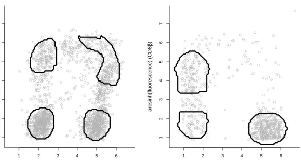
arcsinh(fluorescence) (CD4) arcsinh(fluorescence) (CD8 ββ ) ● ● ● ● ● ● ● ● ● ●● ● ● ● ● ● ●● ● ● ● ● ● ● ● ● ● ● ● ● ● ● ● ● ● ● ● ● ● ● ● ● ● ● ● ● ● ● ● ● ● ● ● ● ● ● ● ● ● ● ● ● ● ● ● ● ● ● ● ● ● ● ● ● ● ● ● ● ● ● ● ● ● ● ● ● ● ●● ● ● ● ● ● ● ● ● ● ● ● ● ● ● ● ● ● ● ● ● ● ● ● ● ● ● ● ● ● ● ● ● ● ● ● ● ● ● ● ● ● ●● ●● ● ● ● ● ● ● ● ● ● ● ● ● ● ● ● ● ● ● ● ● ● ● ● ● ● ● ● ● ● ● ● ● ● ● ● ● ● ● ● ● ● ● ● ● ● ● ● ● ● ● ● ● ● ● ● ● ● ● ● ● ● ● ● ● ● ● ● ● ● ● ● ● ● ● ● ● ● ● ● ● ● ● ● ● ● ● ● ● ● ● ● ● ● ● ● ● ● ● ● ● ● ● ● ● ● ● ● ● ● ● ● ● ● ● ● ● ● ● ● ● ● ● ● ● ● ● ● ● ● ● ● ● ● ● ● ● ● ● ● ● ● ● ● ● ● ● ● ● ● ● ● ● ● ● ● ● ● ● ● ● ● ● ● ● ● ● ● ● ● ● ● ● ● ● ● ● ● ● ● ● ● ● ● ● ● ● ● ● ● ● ● ● ● ● ● ● ● ● ● ● ● ● ● ● ● ● ● ● ● ● ● ● ● ● ● ● ● ● ● ●● ● ● ● ● ● ● ● ● ● ● ● ● ● ● ● ● ● ● ● ● ● ● ● ● ● ● ● ● ● ● ● ●● ● ● ● ● ● ● ● ●● ● ● ● ● ● ● ● ● ● ● ● ● ● ● ● ● ● ● ● ●● ● ● ● ● ● ● ● ● ● ● ● ● ● ● ● ● ● ● ● ● ● ● ● ●● ● ● ● ● ● ● ● ● ● ● ● ● ● ● ● ● ● ● ● ● ● ● ● ● ● ● ● ● ● ● ● ● ● ● ● ● ● ● ● ● ● ● ● ● ● ● ● ● ● ● ● ● ● ● ● ● ● ● ● ● ● ● ● ● ● ● ● ● ● ● ● ● ● ● ● ● ● ● ● ● ● ● ● ● ● ● ● ● ● ● ● ● ● ● ● ● ● ● ● ● ● ● ● ● ● ● ● ● ● ● ● ● ● ● ● ● ● ● ● ● ● ● ● ● ● ● ● ● ● ● ● ● ● ● ● ● ● ● ● ● ● ● ● ● ● ● ● ● ● ● ● ● ● ● ● ● ● ● ● ● ● ● ● ● ● ● ● ● ● ● ● ● ● ● ● ● ● ● ● ● ● ● ● ● ● ● ● ● ● ● ● ● ● ● ●● ● ● ● ● ● ● ● ● ● ● ● ● ● ● ● ● ● ● ● ● ● ● ● ● ● ● ● ● ● ● ● ● ● ● ● ● ● ● ● ● ● ● ● ● ● ● ● ● ● ● ● ● ● ● ● ● ● ● ● ● ● ● ● ● ● ● ● ● ● ● ● ● ● ● ● ● ●● ● 1 2 3 4 5 6 1 2 3 4 5 6 7 control patient arcsinh(fluorescence) (CD4) arcsinh(fluorescence) (CD8 ββ )
Figure 2: Cellular fluorescence measurements, after undergoing the arcsinh transformation, corresponding to antibodies CD4 and CD8β after subsetting on CD3-positive cells. The left panel is data from a patient who develops graft-versus-host disease. The right panel is data from a control patient. Further details about the data are given in Brinkman et al. (2007). The shapes correspond to significant negative density curvature regions using the methodology of Duong, Cowling, Koch and Wand (2008) with the bandwidth chosen via the normal scale rule (4).
Figure 2 is a subset of data from the flow cytometry experiment described in Brinkman et al. (2007). The left panel is cellular fluorescence measurements – corresponding to an-tibodies CD4 and CD8β, after gating on CD3-positive cells – on a patient who develops graft-versus-host disease. The right panel corresponds to a control. The data were collected 32 days after each patient had a blood and marrow transplant. The goal is to identify cell populations that differ between control and disease groups and, hence, constitute valid dis-ease biomarkers, e.g. CD4-positive, CD8β-positive, CD3-positive; where ‘positive’ indicates fluorescence of the relevant antibody above a threshold. The shapes in Figure 2 correspond to regions of high significant negative curvature based on the methodology of Godtliebsen, Marron and Chaudhuri (2002) and refined by Duong, Cowling, Koch and Wand (2008).
The bandwidth matrix is chosen according to the normal scale rule (4) withd=r = 2: ˆ
HNS= (1/2)1/5Σˆn−1/5 (5)
where ˆΣis the sample variance. Since the normal density is close to being the density which gives the largest optimal amount of smoothing given a fixed variance for density estimation (Terrell, 1990), then (5) corresponds approximately to the largest bandwidth matrix which should be considered for curvature estimation. The absence of significant curvature for CD4-positive and CD8β-positive cells in the control patient, despite use of this maximal bandwidth, represents an important clinical difference and gives rise to useful cellular sig-natures for graft-versus-host disease. Using the r = 0 normal scale rule, as illustrated in Table 1, could lead to insufficient smoothing for large sample sizes. In more comprehensive analyses of these data, described in Naumann and Wand (2009), more sophisticated filters for identifying cellular signatures are employed. The normal scale rule for second derivative estimation plays an important role in the initial phases of these filters, identifying candidate modal regions of possible interest. The plots in Figure 2 were computed using theRlibrary featurewhose main function uses (5) as the upper limit on the default bandwidth matrix range.
6
Discussion
Kernel smoothing is a widely used non-parametric method for multivariate density esti-mation. It has the potential to be as equally successful for density derivative estiesti-mation. The relative lack of theoretical development for density derivatives compared to densities has hindered this progress. One obstacle is the specification of higher order derivatives. By writing the rth order array ofrth order differentials as an r-fold Kronecker product of first order differentials, we maintain an intuitive, systematic vectorization of all derivatives. This allows the derivation of the equivalent of standard quantities like MISE and AMISE for kernel density estimators for general derivatives.
The single most important factor in the performance of kernel estimators is the choice of the bandwidth. For density estimation, there is now a solid body of work for reliable bandwidth matrix selection. Using the theoretical simplifications afforded by our vector form derivatives, we can write down an unconstrained data-driven selector based on nor-mal scales. These nornor-mal scale selectors facilitate the quantification of the possible gain in performance in using the unconstrained bandwidth matrices compared to more constrained parametrizations. These selectors are a starting point from which more advanced uncon-strained bandwidth selectors can be now developed, and for the second derivative, they are a starting point from which to estimate modal regions.
Acknowledgments. J. E. Chac´on has been partially supported by Spanish Ministerio de
through a ‘Programme Transversal de Recherches’ grant (PTR No. 218), and M.P. Wand received support from Australian Research Council Grant DP055651. The authors are grateful for the assistance received from Nolwenn Le Meur and Richard White.
A
Appendix: Proofs
A.1 Proof of the results in Section 2
A.1.1 Proof of Theorem 1
Proof of Theorem 1. First notice that we can write E\D⊗rf(x;H) =D⊗rKH∗f(x) =KH∗
D⊗rf(x).Therefore, Z B2(x;H)dx= Z kKH∗D⊗rf(x)−D⊗rf(x)k2dx = trR(D⊗rf) + trRK∗K,H,r(f)−2 trRK,H,r(f),
as it is not difficult to check thatR KH∗D⊗rf(x)KH∗D⊗rf(x)Tdx=RK∗K,H,r(f). About
the variance term, it is clear that
Z V(x;H)dx=n−1 Z EkD⊗rKH(x−X1)k2dx−n−1 Z kED⊗rKH(x−X1)k2dx. (6)
The second integral in the right hand side is easily recognized asRK∗K,H,r(f) also, and for
the first one we have
Z EkD⊗rKH(x−X1)k2dx= tr Z Z D⊗rKH(x−y)D⊗rKH(x−y)Tf(y)dxdy = tr Z D⊗rKH(x)D⊗rKH(x)Tdx = tr h (H−1/2)⊗r Z (D⊗rK)H(x)(D⊗rK)H(x)Tdx(H−1/2)⊗r i = tr h (H−1)⊗r|H|−1/2 Z D⊗rK(z)D⊗rK(z)Tdz i =|H|−1/2tr (H−1)⊗rR(D⊗rK) .
A.1.2 Proof of Theorem 2
Notice that, for a function f: Rd → Rp such that every element in D⊗qf(x) is piecewise
continuous, we can write its Taylor polynomial expansion as
f(x+h) = q X r=0 1 r! Ip⊗(hT)⊗r D⊗rf(x) +o(khkq)1p, x,h∈Rd.
See Baxandall and Liebeck (1986, p. 164). The proof of Theorem 2 then follows from Lemmas 1 and 2 below, together with the bias-variance decomposition of the MSE.
Denote IB2(H) = R B2(x;H)dx and IV(H) = R V(x;H)dx the integrated squared bias and integrated variance of the kernel estimator, respectively, so that we can write MISE(H) = IB2(H) + IV(H).
Lemma 1. Assume that (A1)–(A3) hold. We can expand
IB2(H) = m2(K)2 4 tr h (Idr ⊗vecTH)R(D⊗(r+2)f)(Idr⊗vecH) i +o(tr2H)
Proof. We can writeE\D⊗rf(x;H) =RK(z)D⊗rf(x−H1/2z)dz.Now, make use of a Taylor
expansion to get
D⊗rf(x−H1/2z) =D⊗rf(x)−
Idr ⊗(zTH1/2)D⊗(r+1)f(x)
+12
Idr ⊗(zTH1/2)⊗2D⊗(r+2)f(x) +o(trH)1dr.
Substitute this in the previous formula and use assumption (A3) to obtain B(x;H) = m2(K) 2 Idr⊗ {(vecT Id)(H1/2)⊗2}D⊗(r+2)f(x) +o(trH) = m2(K) 2 Idr ⊗vecT HD⊗(r+2)f(x) +o(trH).
We finish the proof by squaring and integrating the previous expression, taking into account assumption (A2).
Lemma 2. Assume that (A1) holds. We can expand
IV(H) =n−1|H|−1/2tr (H−1)⊗rR(D⊗rK)
+o(n−1|H|−1/2trr(H−1)).
Proof. From the proof of Theorem 1 and the arguments in the previous lemma we have
Z V(x;H)dx=n−1 Z EkD⊗rKH(x−X1)k2dx+O(n−1) =n−1|H|−1/2tr (H−1)⊗rR(D⊗rK) +o(n−1|H|−1/2trr(H−1)).
A.1.3 Proof of Theorem 3
Proof. Similar to the decomposition MISE(H) = IB2(H)+IV(H), we can write AMISE(H) = AIB2(H)+AIV(H) where AIB2(H) and AIV(H) are the leading terms of IB2(H) and IV(H) respectively from Lemmas 1 and 2.
DenoteKr,s∈ Mrs×rsthe commutation matrix of orderr, s; see Magnus and Neudecker
(1979). The commutation matrix allows us to commute the order of the matrices in a Kronecker product e.g., ifA∈ Mn×r and B∈ Mm×s, thenKm,n(A⊗B)Kr,s=B⊗A.
To determine the derivative, we first find the differentials. Differentials of a function
f : Rd → Rp have the advantage that they are always the same dimension as f itself, as
opposed to derivatives whose dimension depends on the order of the derivative. So higher order differentials are easier to manipulate. The first identification theorem of Magnus and
Neudecker (1999, p. 87) states if the differential off(y) can be expressed asdf(y) =A(y)y for some matrix A(y) ∈ Mp×d then the derivative is Df(y) = A(y). The differential of
AIB2(H) is
dAIB2(H) = m2(K)2
4 (vec
T R(D⊗(r+2)f))K⊗2
dr,d2[(Kdr+2,d2 ⊗Idr) +Id2r+4]
×(Id2⊗vecH⊗vecIdr)dvecH
since
dvec{Idr ⊗(vecHvecT H)}=dvec[Kdr,d2{(vecHvecT H)⊗Idr}Kd2,dr]
= (Kdr,d2 ⊗Kdr,d2)dvec{(vecHvecT H)⊗Idr}
=K⊗dr2,d2[(Kdr+2,d2 ⊗Idr) +Id2r+4](Id2⊗vecH⊗vecIdr)dvecH
where the last line follows by using a similar reasoning to determine Equation (11) in the proof of Theorem 2 in Chac´on and Duong (2008).
The differential of AIV(H) is
dAIV(H) =−n12AIV(H)(vecT H−1) +n−1|H|−1/2(vecT R(D⊗rK))(H−1)⊗2r ×Λr[(Idr−1 ⊗Kd,dr−1)(vecH⊗(r−1)⊗Id)⊗Id]
o
dvecH
whereΛr=Pri=1K
⊗2
di,dr−i. The reasoning follows similar lines to computing Equations (9)
and (10) in the proof of Theorem 2 in Chac´on and Duong (2008).
Let every entry ofHbe O(n−β) for β >0. Then dAIV(H) =O(nβ(d/2+r+1)−1) dvecH
and dAIB2(H) = O(n−β) dvecH. Equating powers gives β = 2/(d+ 2r+ 4) and thus
dAMISE(H) = O(n−2/(d+2r+4)) dvecH. The optimal H is a solution of the equation
∂AMISE(H)/(∂vecH) = 0, so all its entries are O(n−2/(d+2r+4)), which implies that minHAMISE(H) =O(n−4/(d+2r+4)).
A.1.4 Proof of Theorem 4
The proof follows directly from Lemmas 1 and 2.
Proof. From Lemma 1, E \D⊗rf(x;H) = D⊗rf(x) + m22(K)(Idr ⊗vecT H)D⊗(r+2)f(x)[1 + O(trH)]. For the variance, we have
VarD\⊗rf(x;H) =n−1D⊗rKHD⊗rKT
H∗f(x)−n
−1[KH∗D⊗rf(x)][KH∗D⊗rf(x)T].
From Lemma 2, the convolution in the first term dominates the convolution in the second term since the value of the former is
D⊗rKHD⊗rKHT ∗f(x) =|H|
−1/2(H−1/2)⊗rR(D⊗rK)(H−1/2)⊗rf(x)[1 +o(1)]
A.2 Proof of the results in Section 3
The proofs in Sections A.2.1 and A.2.2 assume without loss of generality that f = φΣ
to simplify the presentation of the results. These results for the general normal density
f =φΣ(· −µ) remain valid since they are invariant under this translation.
A.2.1 Proof of Theorem 5
The proof of Theorem 5 is based on the exact formula given in Theorem 1. Notice that, in the normal case, we haveRφ∗φ,H,r(φΣ) =Rφ,2H,r(φΣ) and R(D⊗rφΣ) =Rφ,0,r(φΣ), so
that it follows that all we need to have an explicit expression for the MISE function in the normal case is just to obtain explicit formulas for trRφ,H,r(φΣ) and tr (H−1)⊗rR(D⊗rφ)
. These are provided in the following lemma.
Lemma 3. For any symmetric positive definite matrix Hwe have
i) Rφ,H,r(φΣ) = 2d/2+rR(D⊗rφH+2Σ).
ii) tr (H−1)⊗rR(D⊗rφΣ)
= 2−(d+r)π−d/2|Σ|−1/2µ
r(Σ1/2HΣ1/2).
From i) andii) we immediately obtain
iii) trRφ,H,r(φΣ) = (2π)−d/2|H+ 2Σ|−1/2µr(H+ 2Σ).
iv) tr (H−1)⊗rR(D⊗rφ)
= 2−(d+r)π−d/2µ
r(H).
Proof. i) Reasoning as in Chac´on and Duong (2008), it is easy to check that vecR(D⊗rφΣ) = (−1)rD⊗2rφ2Σ(0) = (−1)r2−(d/2+r)D⊗2rφΣ(0).
With this in mind, an element-wise application of some of the results in Appendix C of Wand and Jones (1995) leads to
vecRφ,H,r(φΣ) = vec Z Rd (φH∗D⊗rφΣ)(x)D⊗rφΣ(x)Tdx = vec Z Rd D⊗rφH+Σ(x)D⊗rφΣ(x)Tdx = Z Rd D⊗rφΣ(x)⊗D⊗rφH+Σ(x)dx = (−1)r Z Rd D⊗2rφΣ(x)φH+Σ(x)dx = (−1)rD⊗2rφH+2Σ(0) = 2d/2+rvecR(D⊗rφH+2Σ),
ii) Chac´on and Duong (2008) also show that
vecR(D⊗rφΣ) = 2−(d+r)π−d/2OF(2r)|Σ|−1/2Sd,2r(vecΣ−1)⊗r. (7)
Moreover, it is not hard to check that the symmetrizer matrix fulfillsSd,2rvec[(H−1)⊗r] =
Sd,2r(vecH−1)⊗r. This is because (vecH−1)⊗rcan be obtained form vec[(H−1)⊗r] by
mul-tiplying it by Kronecker products of commutation and identity matrices, and multiplication of this kind of matrices by the symmetrizer matrix has no effect, as seen from part (iv) of Theorem 1 in Schott (2003). Therefore, if z denotes a d-variate vector with standard normal distribution andx=Σ−1/2z, then
tr (H−1)⊗rR(D⊗rφΣ)= vecT[(H−1)⊗r] vecR(D⊗rφΣ)
= 2−(d+r)π−d/2OF(2r)|Σ|−1/2vecT[(H−1)⊗r]Sd,2r(vecΣ−1)⊗r
= 2−(d+r)π−d/2OF(2r)|Σ|−1/2(vecT H−1)⊗rSd,2r(vecΣ−1)⊗r
= 2−(d+r)π−d/2|Σ|−1/2E[(xTH−1x)r]
= 2−(d+r)π−d/2|Σ|−1/2
E[(zTΣ−1/2H−1Σ−1/2z)r],
Here, the fourth line follows from Theorem 1 in Holmquist (1996b).
A.2.2 Proof of Theorem 6
The proof of Theorem 6 starts from the AMISE expression given in Theorem 2. The term appearing in the asymptotic integrated variance was already computed in Lemma 3 above. For the asymptotic integrated squared bias, it is clear that for the normal kernel we have
m2(K) = 1. From (7) and the results in Holmquist (1996a) it follows that
vecR(D⊗rφΣ) = 2−(d+r)π−d/2|Σ|−1/2(Σ−1/2)⊗2rE[z⊗2r]
withz a d-variate standard normal random vector. Or, in matrix form,
R(D⊗rφΣ) = 2−(d+r)π−d/2|Σ|−1/2(Σ−1/2)⊗rE[(zzT)⊗r](Σ−1/2)⊗r.
Therefore, using (Σ−1/2⊗Σ−1/2) vecH= vec(Σ−1/2HΣ−1/2) and some other matrix results from Magnus and Neudecker (1999, p. 48), we come to
tr(Idr⊗vecT H)R(D⊗(r+2)φΣ)(Idr⊗vecH)
= 2−(d+r+2)π−d/2|Σ|−1/2trh
(Σ−1)⊗r⊗(vecBvecT B) E[(zzT)⊗(r+2)]
i
withB=Σ−1/2HΣ−1/2. Now, the trace in the right hand side can be written as
Etr h (Σ−1zzT)⊗r⊗ {vecBvecT B(zzT)⊗2}i=E h trr(Σ−1zzT) tr{vecBvecT(zzTBzzT)}i =E h (zTΣ−1z)r{vecT(zzTBzzT) vecB}i =E h (zTΣ−1z)r(zTBz)2i.
This yields the proof for the AMISE formula.
If we evaluate the AMISE formula in Theorem 6 at H=cΣfor somec >0 we obtain AMISE(cΣ) = 2−(d+r)π−d/2|Σ|−1/2
n−1c−(d+2r)/2µr(Σ) +161c2µr,2(Σ,Id) .
But we will show below that
µr,2(Σ,Id) = (d+ 2r+ 2)(d+ 2r)µr(Σ), (8) leading to AMISE(cΣ) = 2−(d+r)π−d/2|Σ|−1/2µ r(Σ) n−1c−(d+2r)/2+161c2(d+ 2r+ 2)(d+ 2r) .
and this function is minimized by setting
c= 4 (d+ 2r+ 2)n 2/(d+2r+4) .
Therefore, to finish the proof the only thing left is to show equality (8).
This task, however, is harder than it may seem at first sight. It is relatively easy if
Σ=Id because, in this case, it suffices to show that µr+1(Id) = (d+ 2r)µr(Id), and that
is an immediate consequence of the recursive formula (3). Therefore, to show (8) we will need a recursive formula similar to (3), but for the joint momentsµr,s(A,B). To that end,
we first derive a technical lemma.
Lemma 4. Consider the real function gα(t) ≡gα(t;A,B,C) = tr
{B(C+tA)−1}α
for suitable matrices A,B,Cand arbitrary α∈N. Then, thepth derivative of g is given by
gα(p)(t;A,B,C) = (−1)p(α+p−1)! (α−1)! tr
{A(C+tA)−1}p{B(C+tA)−1}α
so thatg(αp)(0;A,B,C) = (−1)p(α(+α−p−1)!1)!tr(AC−1)p(BC−1)α.
Proof. The result is proved by induction on p. For p = 1, noting that the differential of
B(C+tA)−1 isd B(C+tA)−1 =−B(C+tA)−1A(C+tA)−1dt, we have dtr{B(C+tA)−1}α = trd{B(C+tA)−1}α = tr α X i=1 {B(C+tA)−1}i−1·d B(C+tA)−1 · {B(C+tA)−1}α−i =−tr α X i=1 {B(C+tA)−1}i·A(C+tA)−1· {B(C+tA)−1}α−idt =−αtrA(C+tA)−1{B(C+tA)−1}α dt
and we are done. The case of arbitrarypfollows easily by consideringgα(p)(t) = dtdg(p
−1)
The recursive formula forµr,s(A,B) is given in the next theorem.
Theorem 9. We can write
µr,s(A,B) = r X i=0 s−1 X j=0 r i s−1 j (r+s−i−j−1)!2r+s−i−j−1tr(A−(r−i)B−(s−j))µi,j(A,B).
Proof. For ease of notation we will prove the result forµr,s(A−1,B−1); that is, we will show
that, forqA =zTAz and qB =zTBz with z a d-variate standard normal random vector, we have E[qArqBs] = r X i=0 s−1 X j=0 r i s−1 j (r+s−i−j−1)!2r+s−i−j−1tr(Ar−iBs−j)E[qAi q j B].
It is well known that the joint moment generating function ofqA and qB is M(t1, t2) =E[et1qA+t2qB] =|Id−2t1A−2t2B|−1/2,
see Magnus (1986). From that, we can write
E[qrAqsB] =
∂r+sM ∂tr
1∂ts2
(0,0),
so that all we need is to find a recursive formula for the partial derivatives ofM. With the notations of the previous lemma, it is easy to show that
∂M ∂t2
(t1, t2) =M(t1, t2)·g1(t2;−2B,B,Id−2t1A).
This way, using the formulas for the derivatives ofg1and Leibniz formula for the derivatives
of a product, ∂sM ∂ts 2 (t1, t2) = ∂s−1 ∂ts2−1 M(t1, t2)·g1(t2;−2B,B,Id−2t1A) = s−1 X j=1 s−1 j ∂jM ∂tj2 (t1, t2)·g (s−j−1) 1 (t2;−2B,B,Id−2t1A) = s−1 X j=1 s−1 j (s−j−1)!2s−j−1∂ jM ∂tj2 (t1, t2)·tr {B(Id−2t1A−2t2B)−1}s−j = s−1 X j=1 (s−1)! j! 2 s−j−1∂jM ∂tj2 (t1, t2)·gs−j(t1;−2A,B,Id−2t2B).
Now, if we compute therth partial derivative with respect tot1 we have ∂r+sM ∂tr 1∂ts2 (t1, t2) = r X i=0 s−1 X j=1 r i (s−1)! j! 2 s−j−1∂i+jM ∂ti1∂tj2(t1, t2)·g (r−i) s−j (t1;−2A,B,Id−2t2B)
Substituting (t1, t2) in this expression for (0,0) and using again the previous lemma, we get
As a consequence of this result, we finally are able to prove formula (8).
Corollary 7. For any symmetric matrix A we have
µr,2(A,Id) = (d+ 2r+ 2)(d+ 2r)µr(A).
Proof. First, notice that from the previous theorem, taking into account that A0 =Id,
µr,1(A,Id) = r X i=0 r i (r−i)!2r−itr(A−(r−i))µi,0(A,Id) =dµr(A) + r−1 X i=0 r! i!2 r−itr(A−(r−i))µ i(A) = (d+ 2r)µr(A),
where the last equality follows from (3). Using this and Theorem 9,
µr,2(A,Id) = r X i=0 1 X j=0 r i 1 j (r−i−j+ 1)!2r−i−j+1tr(A−(r−i))µi,j(A,Id) = r X i=0 r i (r−i+ 1)!2r−i+1tr(A−(r−i))µi,0(A,Id) + r i (r−i)!2r−itr(A−(r−i))µi,1(A,Id) = r X i=0 r! i!(r−i+ 1)2 r−i+1tr(A−(r−i))µ i(A) + r! i!2 r−itr(A−(r−i))(d+ 2i)µ i(A) = r X i=0 r! i![2(r−i+ 1) +d+ 2i]2 r−itr(A−(r−i))µ i(A) = (d+ 2r+ 2)µr,1(A,Id) = (d+ 2r+ 2)(d+ 2r)µr(A).
The proofs for the exact formulas for the MISE and AMISE for normal mixture densities are derived in the next two sections.
A.2.3 Proof of Theorem 7
Proof. From the proof of Theorem 5, we have that for K = φ, Rφ∗φ,H,r(f) = Rφ,2H,r(f)
and R(D⊗rf) = Rφ,0,r(f). Combining this with Theorem 1 and part iv) of Lemma 3 we
come to
MISE{(D\⊗rf(·;H)}= 2−rn−1(4π)−d/2|H|−1/2µ
where$a = trRφ,aH,r(f) = (vecT Idr) vecRφ,aH,r(f). Now,
vecRφ,aH,r(f) = vec Z φaH∗D⊗rf(x)D⊗rf(x)Tdx = k X `,`0=1 w`w`0 Z D⊗rφΣ`0(x−µ`0)(x)⊗D⊗rφaH+Σ`(x−µ`)dx = k X `,`0=1 w`w`0(−1)rD⊗2rφaH+Σ`+Σ `0(µ`−µ`0)
so that we can write$a =wTΩaw, where Ωa is thek×k matrix with (`, `0) entry given
by (Ωa)`,`0 = (−1)r(vecT Idr)D⊗2rφaH+Σ`+Σ
`0(µ`−µ`0).
The second expression of (Ωa)`,`0 is derived from the following identity in Holmquist (1996a): D⊗2rφΣ(µ) =φΣ(µ)(Σ−1)⊗2rSd,2r r X j=0 (−1)jOF(2j) 2r 2j µ⊗(2r−2j)⊗(vecΣ)⊗j (9)
and using (vecT Idr)(Σ−1)⊗2r= vecT(Σ−2)⊗r.
A.2.4 Proof of Theorem 8
Proof. To determine the AMISE formula, as we already have the integrated variance from Theorem 7, it suffices to find an expression for the asymptotic integrated squared bias
AIB2(H) = 14tr
(Idr ⊗vecTH)R(D⊗(r+2)f)(Idr⊗vecH)
= 14vecT Idr ⊗(vecHvecT H)vecR(D⊗(r+2)f).
We can write vecR(D⊗(r+2)f) = vecRφ,0·H,r+2(f) = k X `,`0=1 w`w`0(−1)r+2D⊗2r+4φΣ`+Σ `0(µ`−µ`0)
so that 4AIB2(H) =wTΩew, withµ``0 =µ`−µ`0,Σ``0 =Σ`+Σ`0,
e
Ω`,`0 = (−1)rvecT Idr ⊗(vecHvecT H)D⊗2r+4φΣ
``0(µ``0) = (−1)rφΣ``0(µ``0) (vecTId)⊗r⊗(vecTH)⊗2 (Σ−``10)⊗(2r+4)Sd,2r+4 × r+2 X j=0 (−1)jOF(2j) 2r+ 4 2j µ``⊗(20 r−2j+4)⊗(vecΣ``0)⊗j = (−1)rφΣ``0(µ``0) (vecTΣ−``20)⊗r⊗(vecT(Σ−``1HΣ−``1))⊗2 Sd,2r+4 × r+2 X j=0 (−1)jOF(2j) 2r+ 4 2j µ⊗``(20 r−2j+4)⊗(vecΣ``0)⊗j, using (9).
A.3 Proof of the results in Section 4
A.3.1 Proof of Corollary 3
Proof. From Theorem 6,HAMISE =cAMISEΣwherecAMISE ={4/[(d+ 2r+ 2)n]}2/(d+2r+4).
Substituting this into the equation immediately following Eq. 8, min H∈FAMISE(H) = 2 −(d+r)π−d/2|Σ|−1/2µ r(Σ)c2AMISE n−1c−AMISE(d+2r+4)/2+ 161(d+ 2r+ 2)(d+ 2r) = 2−(d+r)π−d/2|Σ|−1/2µ r(Σ) 4 d+ 2r+ 2 4/(d+2r+4) ×1 4(d+ 2r+ 2) + 1 16(d+ 2r+ 2)(d+ 2r) n−4/(d+2r+4) = 2−(d+r+4)π−d/2(d+ 2r+ 2)(d+ 2r+ 4) 4 d+ 2r+ 2 4/(d+2r+4) × |Σ|−1/2µr(Σ)n−4/(d+2r+4) = 2−(d+r+4)28/(d+2r+4)π−d/2(d+ 2r+ 4)(d+ 2r+ 2)(d+2r)/(d+2r+4) × |Σ|−1/2µr(Σ)n−4/(d+2r+4).
A.3.2 Proof of Corollary 4
Proof. Substituting H=h2Id into the AMISE formula in Theorem 6,
AMISE(h2Id) = 2−(d+r)π−d/2{n−1h−d−2rµr(Id) +161|Σ|−1/2µr,2(Σ,Σ1/2(h−2Id)Σ1/2)}
= 2−(d+r)π−d/2{n−1h−d−2rµr(Id) +161|Σ|−1/2µr+2(Σ)h4}
sinceµr,2(Σ,Σ) =µr+2(Σ). Differentiating with respect to h and setting to zero
−(d+ 2r)n−1h−d−2r−1µr(Id) +14|Σ|−1/2µr+2(Σ)h3 = 0 gives hAMISE= 4(d+ 2r)|Σ|1/2µ r(Id) µr+2(Σ)n 1/(d+2r+4) .