New Jersey Institute of Technology
Digital Commons @ NJIT
Theses Theses and Dissertations
Spring 2016
Semi supervised weighted maximum variance
dimensionality reduction
Pranitha Surya Andalam New Jersey Institute of Technology
Follow this and additional works at:https://digitalcommons.njit.edu/theses
Part of theComputer Sciences Commons
This Thesis is brought to you for free and open access by the Theses and Dissertations at Digital Commons @ NJIT. It has been accepted for inclusion in Theses by an authorized administrator of Digital Commons @ NJIT. For more information, please [email protected].
Recommended Citation
Andalam, Pranitha Surya, "Semi supervised weighted maximum variance dimensionality reduction" (2016).Theses. 266.
Copyright Warning & Restrictions
The copyright law of the United States (Title 17, United
States Code) governs the making of photocopies or other
reproductions of copyrighted material.
Under certain conditions specified in the law, libraries and
archives are authorized to furnish a photocopy or other
reproduction. One of these specified conditions is that the
photocopy or reproduction is not to be “used for any
purpose other than private study, scholarship, or research.”
If a, user makes a request for, or later uses, a photocopy or
reproduction for purposes in excess of “fair use” that user
may be liable for copyright infringement,
This institution reserves the right to refuse to accept a
copying order if, in its judgment, fulfillment of the order
would involve violation of copyright law.
Please Note: The author retains the copyright while the
New Jersey Institute of Technology reserves the right to
distribute this thesis or dissertation
Printing note: If you do not wish to print this page, then select
“Pages from: first page # to: last page #” on the print dialog screen
The Van Houten library has removed some of the
personal information and all signatures from the
approval page and biographical sketches of theses
and dissertations in order to protect the identity of
NJIT graduates and faculty.
ABSTRACT
SEMI SUPERVISED WEIGHTED MAXIMUM VARIANCE DIMENSIONALITY REDUCTION
by
Pranitha Surya Andalam
In the recent years, we have huge amounts of data which we want to classify with
minimal human intervention. Only few features from the data that is available might be
useful in some scenarios. In those scenarios, the dimensionality reduction methods play a
major role for extracting useful features. The two parameter weighted maximum variance
(2P-WMV) is a generalized dimensionality reduction method of which principal
component analysis (PCA) and maximum margin criterion (MMC) are special cases.. In
this paper, we have extended the 2P-WMV approach from our previous work to a
semi-supervised version. The objective of this work is specially to show how two parameter
version of Weighted Maximum Variance (2P-WMV) performs in Semi-Supervised
environment in comparison to the supervised learning. By making use of both labeled and
unlabeled data, we present our method with experimental results on several datasets using
SEMI SUPERVISED WEIGHTED MAXIMUM VARIANCE DIMENSIONALITY REDUCTION
by
Pranitha Surya Andalam
A Thesis
Submitted to the Faculty of New Jersey Institute of Technology
In Partial Fulfillment of the Requirements for the Degree of Master of Science in Computer Science
Department of Computer Science
APPROVAL PAGE
SEMI SUPERVISED WEIGHTED MAXIMUM VARIANCE DIMENSIONALITY REDUCTION
Pranitha Surya Andalam
Usman Roshan, Advisor Date Associate Professor of Computer Science, NJIT
Zhi Wei, Committee Member Date Associate Professor of Computer Science, NJIT
Dimitri Theodoratos, Committee Member Date Associate Professor of Computer Science, NJIT
BIOGRAPHICAL SKETCH
Author: Pranitha Surya Andalam
Degree: Master of Science
Date: May 2016
Undergraduate and Graduate Education:
• Master of Science in Computer Science
New Jersey Institute of Technology, Newark, NJ, 2016 • Bachelor of Engineering in Computer Science
Chaitanya Bharathi Institute of Technology, Hyderabad, India, 2013
Major: Computer Science
v
I dedicate this Thesis work to my father and mother who have constantly supported me all through my endeavors and special thanks to my brother who has encouraged me and made me realize my inner potential and strengths and who taught me to stand still in the face of challenges. I also extend my thanks to my sister-in-law who has taught me how to be brave and confident. This research would not
have been possible without their support. Their constant well-wishing have made this possible
vi
ACKNOWLEDGMENT
I would like to express my deepest and sincere gratitude to Professor Mr. Usman Roshan
who has paved a way for me and helped me get started in the field of Machine Learning.
He has always been supportive and encouraging in carrying out the research work.
Without his guidance and persistent help, this thesis work would not have been possible.
I would also like to thank my thesis committee members, Professor Mr. Zhi Wei
and Professor Mr. Dimitri Theodoratos for taking time to review my thesis work. Their
feedbacks have been absolutely invaluable.
In addition, I would also like to extend my thanks to PhD student Mohammedreza Esfandiari for his valuable suggestions during my research work.
vii TABLE OF CONTENTS Chapter Page 1. INTRODUCTION………. 1 1.1 Objective……….. 1 1.2 Background Information……….. 1 2. METHODS……….... . 4 2.1 Two Parameter Weighted Maximum Variance Discriminant………. 4
2.2 Semi-Supervised Weighted Maximum Variance……… 5
2.2.1 Nearest Neighbors ………. 6
2.2.2 Majority Among K-Nearest Neighbors ………. 6
2.2.3 K-Means Clustering ………... 7
2.2.3.1 Relative Clustering Validity Criterion ………... 8
3. EXPERIMENTAL PERFORMANCE STUDY ………... 9
3.1 Experimental Methodology………. 11
3.2 Experimental Results Across Datasets……… 14
4. DISCUSSION……….... . 15 5. CONCLUSION……….. . 16 REFERENCES………... 17
viii
LIST OF TABLES
3.1 Datasets from the UCI Machine Learning repository which we used in our
empirical study …..……… 10
3.2 Average cross-validation error on each dataset from UCI machine learning
ix
LIST OF DEFINITIONS
Covariance It is a measure of how much two random variables change together.
Dimensionality Reduction It is the process of reducing the number of random variables under consideration, and can be divided into feature selection and feature extraction.
Discriminant Function When the decision on input x should be made, choose the class with highest value of discriminant function.
Laplacian Matrix It is a matrix representation of a graph. It can be used to calculate the number of spanning trees for a graph.
Scatter-Matrix It is a statistic that is used to make estimates of the covariance matrix.
Semi-Supervised Given both labeled and unlabeled data, one has to find a function that approximates the behavior in generalizable fashion.
Supervised Given the data and labels, one has to find a function that approximates the behavior in generalizable fashion.
Variance It is a measure to define how far each number is from the mean.
x
LIST OF ABBREVIATIONS
1-NN One Nearest Neighbors
2P-WMV Two Parameter Weighted Maximum Variance
2P-SSWMV Two Parameter Semi Supervised Weighted Maximum Variance
EVD Eigen Value Decomposition
MMC Maximum Margin Criterion
PCA Principal Component Analysis
SSWMV Semi – Supervised Weighted Maximum Variance
SVD Singular Value Decomposition
WMMC Weighted Maximum Margin Criterion
1
CHAPTER 1 INTRODUCTION
1.1Objective
The weighted maximum variance is a general procedure for dimensionality reduction of
which principal component analysis and the maximum margin criterion discriminant are
special cases. In Supervised work we studied a simple two parameter version of this that
we call 2P-WMV. There we show that with our extracted features we obtain a lower
average classification error given by 1-nearest neighbor compared to other
dimensionality reduction methods and the raw features. In this paper, we extend two
parameter weighted maximum variance method to work in Semi-Supervised setting. Here
we present the classification accuracies across various datasets using weighted maximum
variance in both supervised and semi-supervised learning, and compare the results. In
semi-supervised version, we use various methods to construct the input data before
extracting features which we will discuss in this research work.
1.2 Background Information
The problem of dimensionality reduction arises in many data mining and machine
learning tasks where we want to extract useful and meaningful features from datasets
with large number of features. Among many such dimensionality reduction methods,
principal component analysis (PCA) [1] is a very popular choice in which data is
measured in terms of its principal components rather than on a normal x-y axis. Principal
2
the data is most spread out. PCA projects data onto lower dimensions by maximizing
their variance without considering their class labels.
Suppose we are given the vector 𝑥𝑖 ∈ 𝑅𝑑 for 𝑖 = 0 … 𝑛 − 1 and a real matrix
𝐶 ∈ 𝑅𝑛×𝑛. Let 𝑋 be the matrix containing 𝑥
𝑖 as its columns (ordered 𝑥0 through 𝑥𝑛−1).
PCA is given by the following equation:
By symbolic manipulation, we obtain PCA discriminant as arg 𝑚𝑎𝑥𝑤 𝑤𝑇𝑆 𝑡w
which is the optimization criterion for PCA where 𝑆𝑡= 1
𝑛∑ (𝑥𝑖 − 𝑚)(𝑥𝑖− 𝑚)
𝑇
𝑖 is the
total scatter matrix.
Maximum Margin Criterion (MMC) is a supervised dimensionality reduction
method that overcomes the limitations of the Linear Discriminant Analysis (LDA) or
Fisher Linear discriminant, which can be applied even when the within-class scatter
matrix is singular and has also shown to achieve higher classification accuracy [2]. MMC
is given by the following equation:
Where 𝐺𝑖𝑗 = 1
𝑛 for all 𝑖 and 𝑗 and 𝐿𝑖𝑗 = 1
𝑛𝑘 if 𝑖 and 𝑗 have class labels k and 0
otherwise. By some symbolic manipulation we obtain the MMC discriminant as
arg 𝑚𝑎𝑥 𝑤 1 2𝑛∑ 1 𝑛(𝑤 𝑇(𝑥 𝑖− 𝑥𝑗))2 𝑖,𝑗 (1.1) arg 𝑚𝑎𝑥 𝑤 1 2𝑛(∑ 𝐺𝑖𝑗(𝑤 𝑇(𝑥 𝑖 − 𝑥𝑗))2 𝑖,𝑗 − ∑ 2𝐿𝑖𝑗(𝑤𝑇(𝑥𝑖 − 𝑥𝑗))2) 𝑖,𝑗 (1.2)
3
𝑤𝑇(𝑆𝑡− 2𝑆𝑤)w where 𝑆𝑡 is the total scatter matrix which can be written as
𝑆𝑡= 𝑆𝑏 + 𝑆𝑤. Here 𝑆𝑏 is the between-class matrix and 𝑆𝑤 is the within-class matrix.
Now consider the optimization problem which is more general representation of
PCA and MMC:
where 𝑤 ∈ 𝑅𝑑.
The above equation can be modified to two parameter weighted maximum
variance (2P-WMV) approach by setting 𝐶𝑖𝑗 = 𝛼 < 0 if 𝑥𝑖 and 𝑥𝑗 have same class label
and 𝐶𝑖𝑗 = 𝛽 > 0 if 𝑥𝑖 and 𝑥𝑗 otherwise. The idea behind this approach is to minimize the
distance between projected pairwise points belonging to the same class and maximize the
distance for points in different class to get better classification accuracies. In
Semi-Supervised case, we use the whole dataset to train the classifier. We use 1-Nearest
Neighbors to predict labels of unclassified data and use those predictions to maximize or
minimize the distance between the pairwise points. We employ singular value
decomposition (SVD) with Graph Laplacians to represent high dimensional data.
We will briefly review two parameter version of WMV [4] and then present the
semi-supervised extension. We compare the two versions on real data with 90%, 50%
and 10% available training data.
arg 𝑚𝑎𝑥 𝑤 1 2𝑛∑ 𝐶𝑖𝑗(𝑤 𝑇(𝑥 𝑖− 𝑥𝑗))2 𝑖,𝑗 (1.3)
4
CHAPTER 2 METHODS
In this Chapter, two parameter weighted maximum variance in supervised and
semi-supervised setting are presented. Consider the generic equation 1.3, which is the general
representation of PCA and MMC. By substituting 𝐶𝑖𝑗 = 𝐺𝑖𝑗 − 2𝐿𝑖𝑗 in equation 1.3, we
obtain the following form of WMV
where 𝐺 ∈ 𝑅𝑛×𝑛 as 𝐺 𝑖𝑗 =
1
𝑛 for all 𝑖 and 𝑗. The above equation is similar to
equation 1.2 i.e., MMC. But 2P-WMV in supervised and semi-supervised learning differs
by definition of 𝐿𝑖𝑗.
2.1 Two Parameter Weighted Maximum Variance Discriminant
When supervised data is available, 𝐿𝑖𝑗 in equation 2.1 can be defined as the following:
where 𝑦𝑖 and 𝑦𝑗 are the labels of 𝑖 and 𝑗 , and 𝐿 ∈ 𝑅𝑛×𝑛.
arg 𝑚𝑎𝑥 𝑤 1 2𝑛(∑ 𝐺𝑖𝑗(𝑤 𝑇(𝑥 𝑖 − 𝑥𝑗))2 𝑖,𝑗 − ∑ 2𝐿𝑖𝑗(𝑤𝑇(𝑥 𝑖 − 𝑥𝑗))2) 𝑖,𝑗 (2.1) 𝐿𝑖𝑗 = { 𝛼 𝑖𝑓 𝑦𝑖 = 𝑦𝑗 𝛽 𝑖𝑓 𝑦𝑖 ≠ 𝑦𝑗 0 𝑖𝑓 𝑦𝑖 𝑜𝑟 𝑦𝑗 𝑖𝑠 𝑢𝑛𝑑𝑒𝑓𝑖𝑛𝑒𝑑 (2.2)
5
This gives us the discriminant (𝑤𝑇(𝑆𝑡− 2(𝛼𝑆𝑤′ + 𝛽𝑆𝑏′))𝑤) where
𝑆𝑤′ = 1 𝑛∑ 𝑛𝑘∑ (𝑥𝑗− 𝑚𝑘)(𝑥𝑗− 𝑚𝑘) 𝑇 𝑐𝑙(𝑥𝑗)=𝑘 𝑐 𝑘=1 𝑆𝑏′ = 1 2𝑛∑ ∑ ∑ (𝑥𝑗− 𝑥𝑗)(𝑥𝑗− 𝑥𝑗) 𝑇 𝑐𝑙(𝑥𝑖)=𝑐,𝑐𝑙(𝑥𝑗)=𝑑 𝑘 𝑑=𝑐+1 𝑐 𝑘=1
The discriminant yielded by 2P-WMV is given by the standard total scatter
matrix, a modified within-class matrix, and a pairwise inter-class scatter matrix. We can
obtain the maximum margin criterion from this by setting 𝛼 = 1
𝑛𝑘 if 𝑦𝑖 = 𝑘, 𝑦𝑗 = 𝑘 and
𝛽 = 0. This discards the inter-class scatter matrix and makes 𝑆𝑤′ = 𝑆𝑤.
2.2 Semi-Supervised Weighted Maximum Variance
In supervised two parameter weighted maximum variance, the method leverages only
labeled data to construct data matrix before finding the Laplacian matrix and their Eigen
value using singular value decomposition (SVD) / Eigen value decomposition (EVD).
In Semi-Supervised learning, both unlabeled and labeled data are available while
extracting features. In this case, we define the matrix 𝐿𝑖𝑗 as
After defining L and G compute 𝐿𝑔 the Laplacian of G, 𝐿𝑙 the Laplacian of L, and
the matrix 1
𝑛𝑋(𝐿𝑔− 𝐿𝑙)𝑋
𝑇 (the SSWMV discriminant). The solution to 2P-WMV is 𝑤
𝐿𝑖𝑗= { 𝛼 𝑖𝑓 𝑦𝑖 = 𝑦𝑗 𝛽 𝑖𝑓 𝑦𝑖 ≠ 𝑦𝑗 𝛼 𝑓𝑜𝑟 𝑢𝑛𝑙𝑎𝑏𝑙𝑒𝑑 𝑝𝑜𝑖𝑛𝑡𝑠 𝑎𝑛𝑑 𝑖𝑓 𝑖 𝑎𝑛𝑑 𝑗 𝑏𝑒𝑙𝑜𝑛𝑔 𝑡𝑜 𝑡ℎ𝑒 𝑠𝑎𝑚𝑒 𝑐𝑙𝑎𝑠𝑠 0 𝑜𝑡ℎ𝑒𝑟𝑤𝑖𝑠𝑒 (2.3)
6
that maximizes 1
𝑛𝑤 𝑇𝑋(𝐿
𝑔− 𝐿𝑙)𝑋𝑇w which is in turn given by the largest eigenvector of 1
𝑛𝑋(𝐿𝑔− 𝐿𝑙)𝑋 𝑇 [5].
Semi-supervised learning is a class of supervised learning tasks and techniques
that also make use of unlabeled data along with labeled data for training. As
Semi-supervised learning is a combination of both labeled and unlabeled data, we need a
mechanism to classify the unlabeled data before constructing the matrix 𝐿𝑖𝑗. We have
experimented with following different approaches to see if the semi-supervised case
performed better than supervised case, with the availability of whole data.
2.2.1 K-Nearest Neighbors
We have employed yet the most simplest and popular approach, K-Nearest Neighbors
(where K=1) to classify unlabeled data by computing their Euclidean distance. By
identifying the 1-Nearest Neighbor for each data point, the 𝐿𝑖𝑗 matrix is constructed
according to the rules in equation 2.2. The idea is to maximize the distance in
between-class scatter matrix and minimize the distance in within-between-class scatter matrix.
2.2.2 Majority among K-Nearest Neighbors
With the above approach, there are many cases where some of the unlabeled data are
wrongly classified with 1-Nearest Neighbors. So in this approach we leveraged the labels
of labeled points and used K-NN to determine the K nearest neighbors for each unlabeled
7
We define the 𝐿𝑖𝑗 matrix as
2.2.3 K-Means Clustering
Given the set of vectors 𝑥𝑖 ϵ 𝑅𝑑 for i = 0…..n – 1, 𝑘 means clustering divides the
n-vectors into 𝑘 (≤ 𝑛) sets 𝑆 = {𝑆1, 𝑆2, 𝑆3… 𝑆𝑘} so as to minimize the distance
within-cluster i.e., each point’s distance to the mean of the within-cluster.
Where 𝜇𝑖is the mean of points in 𝑆𝑖.
We define the matrix 𝐿𝑖𝑗 as
𝐿𝑖𝑗 = { 𝛼 𝑖𝑓 𝑦𝑖 = 𝑦𝑗 𝛽 𝑖𝑓 𝑦𝑖 ≠ 𝑦𝑗 𝛼 𝑢𝑛𝑙𝑎𝑏𝑙𝑒𝑑 𝑝𝑜𝑖𝑛𝑡𝑠 𝑎𝑛𝑑 𝑖𝑓 𝑖 𝑎𝑛𝑑 𝑗 𝑏𝑒𝑙𝑜𝑛𝑔 𝑡𝑜 𝑡ℎ𝑒 𝑠𝑎𝑚𝑒 𝑐𝑙𝑎𝑠𝑠 𝛽 𝑢𝑛𝑙𝑎𝑏𝑙𝑒𝑑 𝑝𝑜𝑖𝑛𝑡𝑠 𝑎𝑛𝑑 𝑖𝑓 𝑖 𝑎𝑛𝑑 𝑗 𝑏𝑒𝑙𝑜𝑛𝑔 𝑡𝑜 𝑑𝑖𝑓𝑓𝑒𝑟𝑒𝑛𝑡 𝑐𝑙𝑎𝑠𝑠𝑒𝑠 0 𝑜𝑡ℎ𝑒𝑟𝑤𝑖𝑠𝑒 (2.4) arg 𝑚𝑎𝑥 𝑆 ∑ ∑ ‖𝑥 −𝜇𝑖‖2 𝑥 ∈ 𝑆𝑖 𝑘 𝑖=1 (2.5) 𝐿𝑖𝑗 = { 𝛼 𝑖𝑓 𝑦𝑖 = 𝑦𝑗 𝛽 𝑖𝑓 𝑦𝑖 ≠ 𝑦𝑗 𝛼 𝑖𝑓 𝑖 𝑎𝑛𝑑 𝑗 𝑏𝑒𝑙𝑜𝑛𝑔 𝑡𝑜 𝑠𝑎𝑚𝑒 𝑐𝑙𝑢𝑠𝑡𝑒𝑟 𝛽 𝑖𝑓 𝑖 𝑎𝑛𝑑 𝑗 𝑏𝑒𝑙𝑜𝑛𝑔 𝑡𝑜 𝑑𝑖𝑓𝑓𝑒𝑟𝑒𝑛𝑡 𝑐𝑙𝑢𝑠𝑡𝑒𝑟 0 𝑜𝑡ℎ𝑒𝑟𝑤𝑖𝑠𝑒 (2.6)
8
Sometimes after the clusters are formed, we would like to determine its quality. One such
criterion that allows us to determine the partition quality is Relative clustering validity
criteria.
2.2.3.1 Relative Clustering Validity Criterion
Relative clustering validity criteria is used to quantitatively measure the quality of data
partitions formed using clustering. One important validation criterion is the silhouette
width criterion [8]. Silhouette width criterion coefficient is calculated using the mean
intra-cluster distance and the mean nearest cluster distance for each sample.
Where 𝑎(𝑖) the measure of how dissimilar is 𝑖 to its own cluster and 𝑏(𝑖) is the
lowest average dissimilarity of 𝑖 to any other cluster. Thus an 𝑆(𝑖) close to one means
that the datum is appropriately clustered and if 𝑆(𝑖) is close to negative one, then it is
more appropriate if it was clustered in its neighboring cluster. An 𝑆(𝑖) near zero means
that the datum is on the border of two natural clusters.
𝑆(𝑖) = { 1 −𝑎(𝑖) 𝑏(𝑖), 𝑖𝑓 𝑎(𝑖) < 𝑏(𝑖) 0, 𝑖𝑓 𝑎(𝑖) = 𝑏(𝑖) 𝑏(𝑖) 𝑎(𝑖)− 1, 𝑖𝑓 𝑎(𝑖) > 𝑏(𝑖) (2.7)
9
CHAPTER 3
EXPERIMENTAL PERFORMANCE STUDY
To evaluate the classification ability of our extracted features from 2P-SSWMV (two
parameter semi-supervised weighted maximum variance) we have used 1-nearest
neighbor (1NN) algorithm. In previous work [4], we found that 2P-WMV extracted
features to have lower average error (with statistical significance) than the other
dimensionality reduction programs such as the weighted maximum margin criterion
(WMMC), principal component analysis (PCA). Here we consider training validation
splits of 90%, 50% and 10% to evaluate the effect of training data size on our method i.e.,
2P-SSWMV and compare it to 2P-WMV. Using the 1-nearest neighbor classification
algorithm, the features extracted from our 2P-SSWMV (where 𝐿𝑖𝑗 matrix is constructed
using the methods discussed in chapter 2 before extracting features) and the previous
2P-WMV [2]. Here we calculate average error rates across 15 randomly selected datasets
10
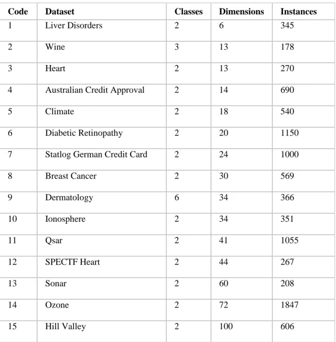
Table 3.1 Datasets from the UCI Machine Learning repository which we used in our empirical study
Code Dataset Classes Dimensions Instances
1 Liver Disorders 2 6 345
2 Wine 3 13 178
3 Heart 2 13 270
4 Australian Credit Approval 2 14 690
5 Climate 2 18 540
6 Diabetic Retinopathy 2 20 1150
7 Statlog German Credit Card 2 24 1000
8 Breast Cancer 2 30 569 9 Dermatology 6 34 366 10 Ionosphere 2 34 351 11 Qsar 2 41 1055 12 SPECTF Heart 2 44 267 13 Sonar 2 60 208 14 Ozone 2 72 1847 15 Hill Valley 2 100 606
Using the above datasets, we have used various methods to construct the
Laplacian matrix and use that matrix for feature extraction using our 2P-SSWMV.
Comparison of the results obtained from 2P-SSWMV and 2P-WMV are shown in Table
11
3.1 Experimental Methodology
In both 2P-WMV and 2P-SSWMV, we let β range from
{-2,-1.9,-1.8,-1.7,-1.6,-1.5,-1.4,-1.3,-1.2,-1.1,-1.0,-0.9,-0.8,-0.7,-0.6,-0.5,-0.4,-0.3,-0.2,-0.1,-0.01} and 𝛼 is fixed to 1. For
all the above datasets, we reduce dimensionality to 5 (we have chosen this value as on an
average for most of the above considered datasets, the Eigen values are negative for
dimensionality greater than 5) which gives the 1NN error on training. Thus the
cross-validation on the training set gives us the best values of β and the reduced number of
12
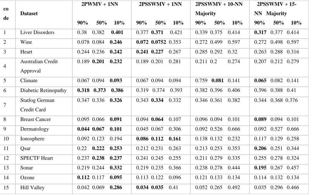
Table 3.2 Average cross-validation error on each dataset from UCI machine learning repository. Shown in bold is lowest error across methods
co de Dataset 2PWMV + 1NN 90% 50% 10% 2PSSWMV + 1NN 90% 50% 10% 2PSSWMV + 10-NN Majority 90% 50% 10% 2PSSWMV + 15-NN Majority 90% 50% 10% 1 Liver Disorders 0.38 0.382 0.401 0.377 0.371 0.421 0.339 0.375 0.414 0.317 0.377 0.414 2 Wine 0.078 0.084 0.246 0.072 0.0752 0.353 0.272 0.499 0.597 0.272 0.498 0.597 3 Heart 0.244 0.236 0.242 0.241 0.227 0.267 0.285 0.292 0.32 0.263 0.288 0.316 4 Australian Credit Approval 0.189 0.201 0.232 0.189 0.201 0.281 0.211 0.2 0.274 0.207 0.212 0.279 5 Climate 0.067 0.094 0.093 0.067 0.094 0.094 0.759 0.081 0.141 0.065 0.082 0.141 6 Diabetic Retinopathy 0.318 0.373 0.386 0.319 0.374 0.393 0.382 0.396 0.406 0.396 0.388 0.41 7 Statlog German Credit Card 0.347 0.336 0.326 0.343 0.334 0.332 0.346 0.361 0.382 0.344 0.368 0.376 8 Breast Cancer 0.095 0.066 0.091 0.094 0.064 0.107 0.096 0.094 0.101 0.089 0.094 0.101 9 Dermatology 0.044 0.067 0.101 0.045 0.067 0.306 0.092 0.526 0.666 0.092 0.527 0.666 10 Ionosphere 0.092 0.123 0.194 0.086 0.112 0.161 0.138 0.132 0.232 0.117 0.129 0.258 11 Qsar 0.22 0.222 0.253 0.212 0.231 0.263 0.213 0.253 0.353 0.206 0.251 0.344 12 SPECTF Heart 0.237 0.238 0.237 0.241 0.245 0.255 0.211 0.279 0.335 0.255 0.278 0.324 13 Sonar 0.219 0.244 0.332 0.219 0.235 0.366 0.238 0.278 0.444 0.195 0.267 0.457 14 Ozone 0.112 0.117 0.095 0.113 0.122 0.096 0.121 0.133 0.134 0.114 0.132 0.134 15 Hill Valley 0.042 0.069 0.286 0.034 0.035 0.41 0.052 0.265 0.492 0.035 0.296 0.466
13
code Dataset
Clustering 90% 50% 10%
2PSSWMV + clustering + relative validity criteria 90% 50% 10%
1 Liver Disorders 0.368 0.386 0.415 0.38 0.395 0.413 2 Wine 0.267 0.309 0.365 0.267 0.309 0.365
3 Heart 0.267 0.237 0.294 0.270 0.244 0.286 4 Australian Credit Approval 0.187 0.214 0.297 0.187 0.214 0.297 5 Climate 0.085 0.087 0.108 0.061 0.088 0.122 6 Diabetic Retinopathy 0.395 0.389 0.424 0.406 0.387 0.42 7 Statlog German Credit Card 0.342 0.377 0.381 0.341 0.38 0.39 8 Breast Cancer 0.096 0.092 0.106 0.095 0.092 0.103 9 Dermatology 0.092 0.157 0.355 0.092 0.157 0.355 10 Ionosphere 0.119 0.131 0.2 0.105 0.135 0.213 11 Qsar 0.215 0.246 0.298 0.211 0.244 0.295 12 SPECTF Heart 0.204 0.249 0.278 0.222 0.277 0.283 13 Sonar 0.2 0.228 0.4 0.214 0.222 0.429 14 Ozone 0.119 0.115 0.111 0.114 0.12 0.113 15 Hill Valley 0.302 0.367 0.49 0.300 0.364 0.49
14
3.2 Experimental Results Across Datasets
The misclassification rate for each training-validation split during cross-validation is
given by
𝑀𝑖𝑠𝑐𝑙𝑎𝑠𝑠𝑖𝑓𝑖𝑐𝑎𝑡𝑖𝑜𝑛 𝑅𝑎𝑡𝑒 = (𝑛𝑢𝑚𝑏𝑒𝑟 𝑜𝑓 𝑚𝑖𝑠𝑐𝑙𝑎𝑠𝑠𝑖𝑓𝑖𝑐𝑎𝑡𝑖𝑜𝑛𝑠
𝑛𝑢𝑚𝑏𝑒𝑟 𝑜𝑓 𝑡𝑒𝑠𝑡𝑠 )
For each 𝛽 value, we considered the mean to be the average cross-validation error
of the splits for that particular validation set and the 𝛽 with minimum error is considered
the optimized 𝛽 for that split. After determining the optimized 𝛽 value, for a given
validation set we extract the features using that 𝛽 and calculate total number of
misclassifications by applying extracted features on the set. In Table 3.2 and 3.3, we
show the cross-validation error on each dataset.
We measure the statistical significance with the Wilcoxon rank test [7]. This is a
standard test to measure the between two methods across a number of datasets. Roughly
speaking it shows the statistical significance between two methods when one outperforms
15
CHAPTER 4 DISCUSSION
Both 2P-SSWMV + 1NN and 2P-WMV + 1NN reduce dimensionality by determining
optimal parameters specific to the given dataset. The two parameter approach is better
than the unsupervised PCA and the non-parametric MMC. In fact 1NN applied to the raw
data can be better than non-parametric MMC most of the time.
In this study, we fixed 𝛼 for 2PWMV and varied only 𝛽. If we cross-validated 𝛼
we could potentially obtain lower error but at the cost of increased running time. In the
current experiments 2P-SSWMV+1NN, 2P-WMV+1NN and WMMC+1NN are the
slowest methods yet still tractable for large datasets.
We chose 1NN as the classification method for this study due to its simplicity and
popularity with dimensionality reduction programs. Other classifiers such as support
vector machines [1] may perform better when replaced with 1NN. However, in that case
the regularization parameter would also need to be optimized via cross-validation which
increases the total runtime.
In this paper, our goal is to show that classification results in Semi-supervised
scenario is more accurate than supervised scenario. However, the results after conducting
experiments using various approaches has shown that semi-supervised could out-perform
16
CHAPTER 5 CONCLUSION
We introduced a two parameter variant of the weighted maximum variance discriminant
in semi-supervised learning and optimize it with cross-validation followed by 1-nearest
neighbor for classification. We have discussed various methods to construct the laplacian
matrix by utilizing data in the entire dataset and used our two parameter variant approach
for reducing dimensionality by feature extraction. Compared to existing dimensionality
reduction approaches, out method obtain the lower average error with statistical
significance across several real datasets from the UCI machine learning repository.
However, semi-supervised version could not do better than supervised version due to
wrongly assigned 𝛼 and 𝛽 values for misclassified data points. Proving semi-supervised
learning is better than supervised learning is a difficult problem. We are continuing our
research to determine ways to identify the classes each pair belongs to which helps to
17
REFERENCES
[1] Alpaydin, E.: Machine Learning. MIT Press, 2004.
[2] Li, H., Jiang, T., Zhang, K.: Efficient and robust feature extraction by maximum margin criterion. In Thurn, S., Saul, L., Scholkopf, B., eds.: Advances in Neural Information Processing Systems 16. MIT Press, Cambridge, MA, 2004.
[3] Chapelle, O., Scholkopf B., Zien, A.: Semi-Supervised Learning. MIT Press, Cambridge, MA, 2006.
[4] Turki, T., Roshan, U.: Weighted maximum variance dimensionality reduction. In Martnez-Trinidad, J., Carrasco-Ochoa, J., Olvera-Lopez, J., Salas-Rodrguez, J., Suen, C., eds.: Pattern Recognition. Volume 8495 of Lecture Notes in Computer Science. Springer International Publishing, 11-20, 2014.
[5] Niijima, S., Okuno, Y.: Laplacian linear discriminant analysis approach to unsupervised feature selection. Computational Biology and Bioinformatics, IEEE/ACM Transactions on 6(4):605- 614, 2009.
[6] Lichman, M.: UCI Machine Learning Repository, 2013.
[7] Kanji, G.K.: 100 Statistical Tests. Sage Publications Ltd, 1999.
[8] Vendramin, L., Campbello, R.J.G.B., Hruschka, E.R.: Relative clustering validity criteria: A comparative overview. Statistical Analysis and Data Mining, 3(4):209-235, 2010.
1
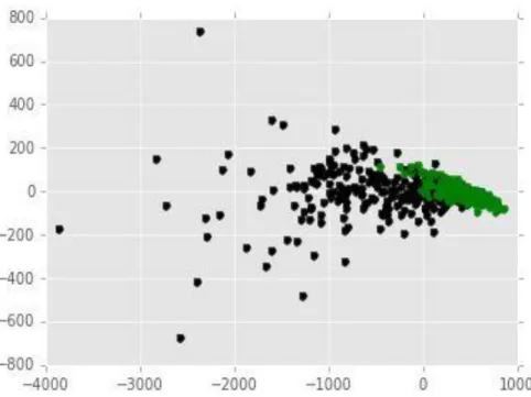
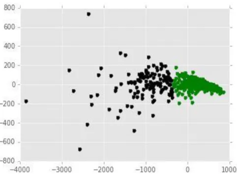
APPENDIX A
VISUALIZATION OF BREAST CANCER DATA
Figure A.1 to A.2 show visualization of breast cancer data on 2-dimensional space
2