Semi-Supervised Novelty Detection
∗Gilles Blanchard [email protected]
Universit¨at Potsdam, Intitut f¨ur Mathematik Am Neuen Palais 10
14469 Potsdam, Germany
Gyemin Lee [email protected]
Clayton Scott [email protected]
Department of Electrical Engineering and Computer Science University of Michigan
1301 Beal Avenue
Ann Arbor, MI 48109-2122, USA
Editor: Ingo Steinwart
Abstract
A common setting for novelty detection assumes that labeled examples from the nominal class are available, but that labeled examples of novelties are unavailable. The standard (inductive) ap-proach is to declare novelties where the nominal density is low, which reduces the problem to density level set estimation. In this paper, we consider the setting where an unlabeled and pos-sibly contaminated sample is also available at learning time. We argue that novelty detection in this semi-supervised setting is naturally solved by a general reduction to a binary classification problem. In particular, a detector with a desired false positive rate can be achieved through a re-duction to Neyman-Pearson classification. Unlike the inductive approach, semi-supervised novelty detection (SSND) yields detectors that are optimal (e.g., statistically consistent) regardless of the distribution on novelties. Therefore, in novelty detection, unlabeled data have a substantial impact on the theoretical properties of the decision rule. We validate the practical utility of SSND with an extensive experimental study.
We also show that SSND provides distribution-free, learning-theoretic solutions to two well known problems in hypothesis testing. First, our results provide a general solution to the general two-sample problem, that is, the problem of determining whether two random samples arise from the same distribution. Second, a specialization of SSND coincides with the standard p-value ap-proach to multiple testing under the so-called random effects model. Unlike standard rejection regions based on thresholded p-values, the general SSND framework allows for adaptation to arbi-trary alternative distributions in multiple dimensions.
Keywords: semi-supervised learning, novelty detection, Neyman-Pearson classification, learning reduction, two-sample problem, multiple testing
1. Introduction
Several recent works in the machine learning literature have addressed the issue of novelty detec-tion. The basic task is to build a decision rule that distinguishes nominal from novel patterns. The learner is given a random sample x1, . . . ,xm∈
X
of nominal patterns, obtained, for example, from acontrolled experiment or an expert. Labeled examples of novelties, however, are not available. The standard approach has been to estimate a level set of the nominal density (Sch¨olkopf et al., 2001; Steinwart et al., 2005; Scott and Nowak, 2006; Vert and Vert, 2006; El-Yaniv and Nisenson, 2007; Hero, 2007), and to declare test points outside the estimated level set to be novelties. We refer to this approach as inductive novelty detection.
In this paper we incorporate unlabeled data into novelty detection, and argue that this frame-work offers substantial advantages over the inductive approach. In particular, we assume that in addition to the nominal data, we also have access to an unlabeled sample xm+1, . . . ,xm+nconsisting
potentially of both nominal and novel data. We assume that each xi, i=m+1, . . . ,m+n is paired
with an unobserved label yi∈ {0,1}indicating its status as nominal (yi=0) or novel (yi=1), and
that(xm+1,ym+1), . . . ,(xm+n,ym+n)are realizations of the random pair(X,Y)with joint distribution
PXY. The marginal distribution of an unlabeled pattern X is the contamination model
X ∼PX = (1−π)P0+πP1,
where Py, y=0,1, is the conditional distribution of X|Y =y, andπ=PXY(Y =1)is the a priori
probability of a novelty. Similarly, we assume x1, . . . ,xm are realizations of P0. We assume no
knowledge of PX, P0, P1, orπ, although in Section 6 (where we want to estimate the proportionπ)
we do impose a natural condition on P1that ensures identifiability ofπ.
We take as our objective to build a decision rule with a small false negative rate subject to a fixed
constraintα on the false positive rate. Our emphasis here is on semi-supervised novelty detection
(SSND), where the goal is to construct a general detector that could classify an arbitrary test point. This general detector can of course be applied in the transductive setting, where the goal is to predict the labels ym+1, . . . ,ym+nassociated with the unlabeled data. Our results extend in a natural way to
this setting.
Our basic contribution is to develop a general solution to SSND by a surrogate problem related to Neyman-Pearson (NP) classification, which is the problem of binary classification subject to a
user-specified constraint α on the false positive rate. In particular, we argue that SSND can be
addressed by applying a NP classification algorithm, treating the nominal and unlabeled samples
as the two classes. Even though a sample from P1 is not available, we argue that our approach
can effectively adapt to any novelty distribution P1, in contrast to the inductive approach which is
only optimal in certain extremely unlikely scenarios. That is, by solving the surrogate problem, we obtain a classifier f such that, up to a tolerance that shrinks as sample sizes increase, P1(f(X) =0) is minimal, while P0(f(X) =1)≤α.
Our learning reduction allows us to import existing statistical performance guarantees for Neyman-Pearson classification (Cannon et al., 2002; Scott and Nowak, 2005) and thereby deduce generaliza-tion error bounds, consistency, and rates of convergence for novelty detecgeneraliza-tion. In addigeneraliza-tion to these theoretical properties, the reduction to NP classification has practical advantages, in that it allows essentially any algorithm for NP classification to be applied to SSND.
that novelties are rare, that is, that πis very small, as in anomaly detection. However, SSND is applicable to anomaly detection provided n is sufficiently large.
We also discuss estimation ofπand the special case ofπ=0, which is not treated in our initial
analysis. We present a hybrid approach that automatically reverts to the inductive approach when
π=0, while preserving the benefits of the NP reduction when π>0. In addition, we describe
a distribution-free one-sided confidence interval forπ, consistent estimation of π, and testing for
π=0, which amounts to a general version of the two-sample problem in statistics. We also discuss
connections to multiple testing, where we show that SSND generalizes a standard approach to mul-tiple testing, based on thresholding p-values, under the common “random effects” model. Whereas the p-value approach is optimal only under strong assumptions on the alternative distribution, SSND can optimally adapt to arbitrary alternatives.
The paper is structured as follows. After reviewing related work in the next section, we present the general learning reduction to NP classification in Section 3, and apply this reduction in Section 4 to deduce statistical performance guarantees for SSND. Section 5 presents our hybrid approach,
while Section 6 applies learning-theoretic principles to inference on π. Connections to multiple
testing are developed in Section 7. Experiments are presented in Section 8, while conclusions are discussed in the final section. Shorter proofs are presented in the main text, and longer proofs appear in the first appendix.
2. Related Work
Inductive novelty detection: Described in the introduction, this problem is also known as one-class classification (Sch¨olkopf et al., 2001) or learning from only positive (or only negative) examples. The standard approach has been to assume that novelties are outliers with respect to the nominal distribution, and to build a novelty detector by estimating a level set of the nominal density (Scott and Nowak, 2006; Vert and Vert, 2006; El-Yaniv and Nisenson, 2007; Hero, 2007). As we discuss below, density level set estimation is equivalent to assuming that novelties are uniformly distributed
on the support of P0. Therefore these methods can perform arbitrarily poorly (when P1is far from
uniform, and still has significant overlap with P0). In Steinwart et al. (2005), inductive novelty
detection is reduced to classification of P0 against P1, wherein P1 can be arbitrary. However an
i.i.d. sample from P1 is assumed to be available in addition to the nominal data. In contrast, the
semi-supervised approach optimally adapts to P1, where only an unlabeled contaminated sample is
available besides the nominal data. In addition, we address estimation and testing of the proportion of novelties.
Classification with unlabeled data: In transductive and semi-supervised classification, labeled training data{(xi,yi)}mi=1from both classes are given. The setting proposed here is a special case where training data from only one class are available. In two-class problems, unlabeled data typ-ically have at best a slight effect on constants, finite sample bounds, and rates (Rigollet, 2007; Lafferty and Wasserman, 2008; Ben-David et al., 2008; Singh et al., 2009), and are not needed for consistency. In contrast, we argue that for novelty detection, unlabeled data are essential for these desirable theoretical properties to hold.
al-though in our context we tend to think of nominal examples as negative. Terminology aside, a number of algorithms have been developed, which we now relate to the present work.
One class of algorithms proceeds roughly as follows: First, identify unlabeled points for which
it seems highly likely that yi=1. Second, learn a classifier from the known positive examples and
the supposed negative examples. Use it on the unlabeled data to update the group of candidates for the negative class and repeat until a stable labeling is reached. Several such algorithms are reviewed in Zhang and Lee (2005) and Zhang and Zuo (2008), but they tend to be heuristic in nature and sensitive to the initial choice of negative examples.
A theoretical analysis of LPUE is provided by Denis (1998); Denis et al. (2005) from the view-point of probably approximately correct (PAC) learnable classes. In PAC learnability, the objective is to find specific classes of classifiers such that the optimal classifier in that class can be approx-imated arbitrarily well, and where the number of samples required is polynomial in the inverse of the error tolerance. While some ideas are common with the present work (such as classifying the nominal sample against the contaminated sample as a proxy for the ultimate goal), our point of view is relatively different and based on statistical learning theory. In particular, our input space can be
non-discrete and we assume the distributions P0 and P1can overlap, which leads us to use the NP
classification setting and study universal consistency properties.
Several other approaches have been developed which, either explicitly or implicitly, rely on a reduction to a classification problem. Steinberg and Cardell (1992) and Ward et al. (2009) propose
frameworks based on logistic regression, but both assume thatπis known. Elkan and Noto (2008)
assume a particular sampling scheme where m and n are related in such a way thatπcan be readily
estimated. Unfortunately, this sampling assumption is not valid in many applications of interest. All three of these works derive their algorithms by a consideration of posterior probabilities, and
consequently they require thatπis known or can be estimated. In contrast, our approach adopts the
(non-Bayesian) Neyman-Pearson criterion and in no way depends on the ability to know or estimate
π.
The idea of reducing LPUE to a binary classification problem has also been treated by Zhang and Lee (2005), Liu et al. (2002), Lee and Liu (2003) and Liu et al. (2003). Most notably, Liu et al. (2002) provide sample complexity bounds for VC classes for the learning rule that minimizes the number of false negatives while controlling the proportion of false positives at a certain level. Our approach extends theirs in several respects. First, Liu et al. (2002) does not consider approximation error or consistency, nor do the bounds established there imply consistency. In contrast, we present a general reduction that is not specific to any particular learning algorithm, and can be used to deduce consistency or rates of convergence. Our work also makes several contributions not addressed
previously in the LPUE literature, including our results relating to the caseπ=0, to the estimation
ofπ, and to multiple testing.
We also note recent work by Smola et al. (2009) described as relative novelty detection. This work is presented as an extension of standard one-class classification to a setting where a reference measure (indicating regions where novelties are more likely) is known through a sample. In practice, the authors take this sample to be a contaminated sample consisting of both nominal and novel measurements, so the setting is the same as ours. The emphasis in this work is primarily on a new kernel method, whereas our work features a general learning reduction and learning theoretic analysis.
discuss in detail the relation of our contamination model to the random effects model, a standard model in multiple testing. We show how SSND is, in several respects, a generalization of that model, and includes several different extensions proposed in the recent multiple testing literature. The SSND model, and the results presented in this paper, are thus relevant to multiple testing as well, and suggest an interesting point of view to this domain. In particular, through a reduction to classification, we introduce broad connections to statistical learning theory.
3. The Fundamental Reduction
To begin, we first consider the population version of the problem, where the distributions are known completely. Recall that PX = (1−π)P0+πP1is the distribution of unlabeled test points. Adopting a hypothesis testing perspective, we argue that the optimal tests for H0: X ∼P0vs. H1: X∼P1are
identical to the optimal tests for H0: X∼P0vs. HX : X∼PX. The former are the tests we would
like to have, and the latter are tests we can estimate by treating the nominal and unlabeled samples as labeled training data for a binary classification problem.
To offer some intuition, we first assume that Py has density hy, y=0,1. According to the
Neyman-Pearson Lemma (Lehmann, 1986), the optimal test with size (false positive rate) α for
H0: X∼P0vs. H1: X∼P1is given by thresholding the likelihood ratio h1(x)/h0(x)at an appropriate value. Similarly, letting hX = (1−π)h0+πh1 denote the density of PX, the optimal tests for H0:
X∼P0vs. HX : X∼PX are given by thresholding hX(x)/h0(x). Now notice
hX(x)
h0(x) = (1−π) +π
h1(x)
h0(x).
Thus, the likelihood ratios are related by a simple monotone transformation, providedπ>0.
Fur-thermore, the two problems have the same null hypothesis. Therefore, by the theory of uniformly
most powerful tests (Lehmann, 1986), the optimal test of size αfor one problem is also optimal,
with the same sizeα, for the other problem. In other words, we can discriminate P0 from P1 by discriminating between the nominal and unlabeled distributions. Note the above argument does not require knowledge ofπother thanπ>0.
The hypothesis testing perspective also sheds light on the inductive approach. In particular, estimating the nominal level set{x : h0(x)≥λ}is equivalent to thresholding 1/h0(x)at 1/λ. Thus, the density level set is an optimal decision rule provided h1 is constant on the support of h0. This
assumption that P1is uniform on the support of P0 is therefore implicitly adopted by a majority of
works on novelty detection.
We now drop the requirement that P0 and P1 have densities. Let f :Rd → {0,1} denote a
classifier. For y=0,1, let
Ry(f):=Py(f(X)6=y)
denote the false positive rate (FPR) and false negative rate (FNR) of f , respectively. For greater generality, suppose we restrict our attention to some fixed set of classifiers
F
(possibly the set of allclassifiers). The optimal FNR for a classifier of the class
F
with FPR≤α, 0≤α≤1, isR∗1,α(
F
) := inff∈F R1(f) (1)
Similarly, introduce
RX(f) := PX(f(X) =0)
= πR1(f) + (1−π)(1−R0(f))
and let
R∗X,α(
F
) := inff∈F RX(f) (2)
s.t. R0(f)≤α.
In this paper we will always assume the following property (involving
F
,P0and P1) holds:(A) For anyα∈(0,1), there exists f∗∈
F
such that R0(f∗) =αand R1(f∗) =R∗1,α(F
).Remark. This assumption is in particular satisfied if the class
F
is such that for any f ∈F
with R0(f)<α, we can find another classifier f′∈F
with R0(f′) =αand f′≥f (so that R1(f′)≤R1(f)). When P0 is absolutely continuous with respect to Lebesque measure, this property can be easily verified for many common classifier sets, for example linear classifiers, decision trees or radial basis function classifiers.
Even without any assumptions on the distribution, it is possible to ensure that (A) is satisfied provided one extends the class
F
to a larger class containing randomized classifiers obtained by convex combination of classifiers of the original class. This construction is standard in the receiver operating characteristic (ROC) literature. Some basic results on this topic are recalled in Appendix B in relation to the above assumption.By the following result, the optimal classifiers for problems (1) and (2) are the same. Further-more, one direction of this equivalence also holds in an approximate sense. In particular,
approx-imate solutions to X ∼P0 vs. X ∼PX translate to approximate solutions for X∼P0 vs. X ∼P1.
The following theorem constitutes our main learning reduction in the sense of Beygelzimer et al. (2005):
Theorem 1 Assume property (A) is satisfied. Consider anyα, 0≤α≤1 , and assumeπ>0 . Then for any f ∈
F
the two following statements are equivalent:(i) RX(f) =R∗X,α(
F
)and R0(f)≤α. (ii) R1(f) =R∗1,α(F
)and R0(f) =α.More generally, let L1,α(f,
F
) =R1(f)−R∗1,α(F
)and LX,α(f,F
) =RX(f)−R∗X,α(F
)denote the excess losses (regrets) for the two problems, and assumeπ>0. If R0(f)≤α+εforε≥0, thenL1,α(f,
F
)≤π−1(LX,α(f,F
) + (1−π)ε).Proof . For any classifier f , we have the relation RX(f) = (1−π)(1−R0(f)) +πR1(f). We start with proving(ii)⇒(i). Consider f ∈
F
such that R1(f) =R∗1,α(F
)and R0(f) =α, but assume RX(f)>R∗X(F
). Let f′∈F
such that RX(f′)<RX(f)and R0(f′)≤α. Then sinceπ>0 ,R1(f′) =π−1 RX(f′)−(1−π)(1−R0(f′))
<π−1(RX(f)−(1−π)(1−α))
contradicting minimality of R1(f).
To establish the converse implication, consider f ∈
F
such that RX(f) =RX∗,α(F
) and R0(f)≤α, but assume R1(f)>R∗1,α(
F
)or R0(f)<α. Let f′be such that R0(f′) =αand R1(f′) =R∗1(F
), whose existence is ensured by assumption (A). ThenRX(f′) = (1−π)(1−α) +πR1(f′)
< (1−π)(1−R0(f)) +πR1(f)
= RX(f),
contradicting minimality of RX(f). To prove the final statement, first note that we established
R∗X,α(
F
) =πR1,∗α(F
) + (1−π)(1−α),by the first part of the theorem. By subtraction we have L1,α(f,F
) = π−1(LX,α(f,F
) + (1−π)(R0(f)−α))≤ π−1(LX,α(f,
F
) + (1−π)ε).Theorem 1 suggests that we may estimate the solution to (1) by solving a surrogate binary classification problem, treating x1, . . . ,xmas one class and xm+1, . . . ,xm+nas the other.
In the rest of the paper, we explore the consequences of this reduction from a theoretical as well as practical perspective. In the next section, we illustrate on the theoretical side, in the case of an empirical risk minimization (ERM) type algorithm, how a finite sample bound for NP classification translates to a finite sample bound for SSND and leads to desirable properties such as consistency. On the other hand, algorithms we can analyze (such as ERM) often do not have the best performance on actual data, and may be computationally infeasible (a situation that is not specific to SSND). Thus in the experimental Section 8 we implement a different method, namely simple but effective schemes based on kernel density estimates. It is important to observe that Theorem 1 still applies to these methods since it just compares two objective functions and is agnostic to the method used.
4. Statistical Performance Guarantees
We now illustrate how Theorem 1 leads to performance guarantees for SSND. We consider the case
of a fixed set of classifiers
F
having finite VC-dimension (Vapnik, 1998), and the NP classificationalgorithm
b
fτ=arg min
f∈F
b
RX(f)
s.t. Rb0(f)≤α+τ, based on (constrained) empirical risk minimization, where
b
RX(f) =
1 n
m+n
∑
i=m+11{f(xi)=16 }, Rb0(f) = 1 m
m
∑
i=11{f(xi)6=0}.
performance). Then we have the following result bounding the difference of the quantities Ri and
Qito their optimal values over
F
:Theorem 2 Assume x1, . . . ,xmand xm+1, . . . ,xm+nare i.i.d. realizations of P0and PX, respectively,
and that the two samples are independent of each other. Assumeπ>0. Let
F
be a set of classifiers of VC-dimension V . Assume property (A) is satisfied and denote by f∗an optimal classifier inF
with respect to the criterion in (1). Fixing δ>0, defineεk=
q
V log k−logδ
k . There exist absolute
constants c,c′such that, if we chooseτ=cεn, the following bounds hold with probability 1−δ:
R0(bfτ)−α ≤ c′εn; (3)
R1(bfτ)−R1(f∗) ≤ c′π−1(εn+εm); (4)
Qi(f∗)−Qi(fbτ) ≤
c′
P(f∗(X) =i)(εn+εm),i=0,1. (5)
The proof is given in Appendix A. The primary technical ingredients in the proof are Theorem 3 of Scott and Nowak (2005) and the learning reduction of Theorem 1 above. The above theorem
shows that the procedure is consistent inside the class
F
for all criteria considered, that is, thesequantities decrease (resp. increase) asymptotically to their value at f∗. This is in contrast to the
statistical learning bounds previously obtained (Liu et al., 2002, Thm. 2), which do not imply consistency.
Following Scott and Nowak (2005), by extending suitably the argument and the method in the
spirit of structural risk minimization over a sequence of classes
F
khaving the universalapproxima-tion property, we can conclude that this method is universally consistent (that is, relevant quantities
converge to their value at f∗, where f∗ is the solution of (1) over the set of all possible
classi-fiers). Therefore, although technically simple, the reduction result of Theorem 1 allows us to deduce stronger results than the existing ones concerning this problem. This can be paralleled with the re-sult that inductive novelty detection can be reduced to classification against uniform data (Steinwart et al., 2005), which made the statistical learning study of that problem significantly simpler.
It is interesting to note that the multiplicative constant in front of the rate of convergence of the precision criteria is PX(f∗(X) =i)−1 rather thanπ−1 for R1. In particular PX(f∗(X) =0)≥
(1−π)(1−α), so that the convergence rate for class 0 precision is not significantly affected as
π→0 . Similarly PX(f∗(X) =1)≥(1−π)α, so the convergence rate for class 1 precision depends
more crucially on the (known)αthan onπ.
For completeness, we briefly discuss the optimality of Qi(f∗)in (5) in the sense of the criterion
Qiitself. Under an additional minor condition, it is possible to show (the details are given at the end
of Appendix B) that under the constraint R0(f)≤α, the best attainable precision for class 0 in the set
F
is attained by f = f∗. Therefore, in (5) (i=0), we are really comparing the precision of bfτ against the best possible class 0 precision given the FPR constraint. On the other hand, it does notmake sense to consider the best attainable class 1 precision under an upper constraint on R0, since
we can have both R0→0 and Q1→1 by only rejecting a vanishingly small proportion of very sure
novelties. But it can easily be seen that f∗ realizes the best attainable class 1 precision under the
equality constraint R0(f) =α.
analogous transductive result is easily obtained by incorporating an additional uniform deviation bound relating the empirical error rates on the unlabeled data to the true error rates.
5. The Caseπ=0 and a Hybrid Method
The preceding reduction of SSND to NP classification is only justified whenπ>0. Aside from
the analysis breaking down, this can be seen as follows. The unlabeled sample is a draw from PX = (1−π)P0+πP1. Whenπ=0, the unlabeled sample is a draw from P0. Therefore it contains
no information about P1. Were we to solve the surrogate NP problem, we would be attempting to
classify between two identical distributions, and the best we could do would be random guessing.
This is confirmed in Table 2 (caseπ=0) where the AUC values for SSND are near one half. Our
goal in this section is to develop a learning reduction, and a parallel result to Theorem 1 in Section
3, but which handles the caseπ=0 more sensibly.
Whenπ=0, we have no information about P1in either sample. Therefore, the only way to get
any traction on the problem is to make some assumption about P1. The inductive method makes
such an assumption (as noted previously in the paper), namely, that P1is uniform on the support of
P0. Since uniformity is the standard assumption without any additional prior knowledge, we aim to
develop a method that performs at least as well as the inductive method whenπ=0.
Therefore we ask the following question: Can we devise a method which, having no knowledge
ofπ, shares the properties of the learning reduction of Section 3 when π>0, and the inductive
approach otherwise? Our answer to the question is “yes” under fairly general conditions.
The intuition behind our approach is the following. The inductive approach to novelty detection performs density level set estimation. Furthermore, as we saw in Section 3, density level sets are optimal decision regions for testing the nominal distribution against a uniform distribution. There-fore, level set estimation can be achieved by generating an artificial uniform sample and performing weighted binary classification against the nominal data (this idea has been developed in more detail by Steinwart et al., 2005). Our approach is to sprinkle a vanishingly small proportion of uniformly distributed data among the unlabeled data, and then implement SSND using NP classification on
this modified data. Whenπ=0, the uniform points will influence the final decision rule to perform
level set estimation. Whenπ>0, the uniform points will be swamped by the actual novelties, and
the optimal detector will be estimated.
To formalize this approach, let 0<pn<1 be a sequence tending to zero. Assume that S is a
compact set which is known to contain the support of P0(obtained, e.g., through support estimation
or through a priori information on the problem), and let P2be the uniform distribution on S. Consider
the following procedure: Let k∼binom(n,pn). Draw k independent realizations from P2, and
redefine xm+1, . . . ,xm+kto be these values. (In practice, the uniform data would simply be appended
to the unlabeled data, so that information is not erased. The present procedure, however, is slightly simpler to analyze.)
The idea now is to apply the SSND learning reduction from before to this modified unlabeled data. Toward this end, we introduce the following notations. For simplicity, we do not explicitly
indicate the underlying class
F
. We refer to any data point that was drawn from either P1 or P2as an operative novelty. The proportion of operative novelties in the modified unlabeled sample is ˜
˜
R∗X,αbe defined in terms of P2,P1, and ˜˜ PX, respectively, in analogy to the definitions in Section 3.
Also denote L2,α(f) =R2(f)−R∗2,α, ˜L1,α(f) =R˜1(f)−R˜∗1,α, and ˜LX,α=R˜X(f)−R˜∗X,α.
By applying Theorem 1 to the modified data, we immediately conclude that if R0(f)≤α+ε,
then
˜L1,α(f)≤1 ˜
π(˜LX,α(f) + (1−π)ε) =˜ 1 ˜
π(˜LX,α(f) + (1−π)(1−pn)ε). (6)
By previously cited results on Neyman-Pearson classification, the quantities on the right-hand side can be made arbitrarily small as m and n grow. The following result translates this bound to the kind of guarantee we are seeking.
Theorem 3 Assume (A) holds. Let f be a classifier with R0(f)≤α+ε. Ifπ=0, then L2,α(f)≤p−n1(˜LX,α(f) + (1−pn)ε).
Ifπ>0, then
L1,α(f)≤ 1
π(1−pn)
(˜LX,α(f) + (1−π)(1−pn)ε+pn).
To interpret the first statement, note that L2,α(f) is the inductive regret. The bound implies that L2,α(f)→0 as long as bothε=R0(f)−αand ˜LX,α(f)tend to zero faster than pn. This suggests
taking pn to be a sequence tending to zero slowly. The second statement is similar to the earlier
result in Theorem 1, but with additional factors of pn. These factors suggest choosing pntending to
zero rapidly, in contrast to the first statement, so in practice some balance should be struck.
Proof Ifπ=0, then ˜L1,α=L2,α and the first statement follows trivially from (6). To prove the second statement, denoteβn:=π(1−π˜pn), and observe that
˜
R∗1,α = inf
R0(f)≤α
˜ R1(f)
= inf
R0(f)≤α
[βnR1(f) + (1−βn)R2(f)]
≤ βnR∗1,α+ (1−βn).
Therefore
˜L1,α(f) = R1˜ (f)−R˜∗1,α
≥ βnR1(f) + (1−βn)R2(f)−βnR∗1,α−(1−βn)
≥ βn(R1(f)−R∗1,α)−(1−βn)
= βnL1,α(f)−(1−βn)
and we conclude, still using (6),
L1,α(f) ≤ 1
βn
˜L1,α+ 1−βn
βn
≤ 1
π(1−pn)
Like Theorem 1, Theorem 3 is quite general, and has both theoretical and practical implications. Theoretically, it could be combined with specific, analyzable algorithms for Neyman-Pearson clas-sification to yield novelty detectors with performance guarantees, as was illustrated in Section 4. We do not develop this theoretical direction here. Practically, any algorithm for Neyman-Pearson clas-sification that generally works well in practice can be applied in the hybrid framework to produce
novelty detectors that perform well for values ofπthat are zero or very near zero. We implement
this idea in the experimental section below.
We also remark that this hybrid procedure could be applied with any prior distribution on nov-elties besides uniform. In addition, the hybrid approach could also be practically useful when n is small, assuming the artificial points are appended to the unlabeled sample.
6. Estimatingπand Testing forπ=0
In the previous sections, our main goal was to find a good classifier function for the purpose of novelty detection. Besides the detector itself, it is often relevant to the user to have an estimate
or bound on the proportionπ of novelties in the contaminated distribution PX. Estimation of π
allows for estimating and optimizing the misclassification rate on the unlabeled data, which is often
of interest in the LPUE literature (see Sec. 2). Estimation of πis also useful for estimating the
precision (as defined in Section 4); this topic will be revisited in the next section in the context of multiple testing.
It may also be useful to test whether there are novelties at all; in other words, since the learnt
detector bf is allowed a certain proportion of false positives, it is important to assess whether the
reported novelties are a statistically significant indication of the presence of true novelties, or if they are likely to be all false positives. We focus on these issues in the present section.
It should first be noted that without additional assumptions,πis not an identifiable parameter in our model. To see this, consider the idealized case where we have an infinite amount of nominal and
contaminated data, so that we have perfect knowledge of P0and PX. Assuming the decomposition
PX = (1−π)P0+πP1 holds, note that any alternate decomposition of the form PX = (1−π−
γ)P0+ (π+γ)P1′, with P1′ = (π+γ)−1(πP1+γP0), andγ∈[0,1−π], is equally valid. Because the
most important feature of the model is that we have no direct knowledge of P1, we cannot decide
which representation is the “correct” one; we could not even exclude a priori the case whereπ=1
and P1 =PX (while producing the exact same observed data) . The previous results established
in Theorems 1-3 are valid for whatever underlying representation is assumed to be correct. For
the estimation of the proportion of novelties, however, it makes sense to define πas the minimal
proportion of novelties that can explain the difference between P0 and PX. First we introduce the
following definition:
Definition 4 Assume P0, P1 are probability distributions on the measure space (
X
,S). We call P1 a proper novelty distribution with respect to P0 if there exists no decomposition of the form P1= (1−γ)Q+γP0where Q is some probability distribution and 0<γ≤1 .This defines a proper novelty distribution P1as one that cannot be confounded with P0; it cannot be
represented as a (nontrivial) mixture of P0with another distribution.
The next result establishes a canonical decomposition of the contaminated distribution into a
mixture of nominal data and proper novelties. As a consequence the proportionπ∗of proper
given the knowledge of the nominal and contaminated distributions (except for the special case P0=PX, where of course the novelty distribution is not defined).
Proposition 5 Assume P0, PX are probability distributions on the measure space(
X
,S). If PX 6=P0, there is a uniqueπ∗∈(0,1]and P1 such that the decomposition PX = (1−π∗)P0+π∗P1holds, and such that P1is a proper novelty distribution with respect to P0. If we additionally defineπ∗=0 when PX =P0, then in all cases,
π∗:=min{α∈[0,1]:∃Q probability distribution: P
X= (1−α)P0+αQ}. (7)
The proof is given in Appendix A. For the rest of this section we assume for simplicity of
notation thatπand P1are the proportion and distribution of proper novelties of PX with respect to
P0. The results to come are also informative for improper novelty distributions, in the following
sense: if P1is not a proper novelty distribution and the decomposition PX = (1−π)P0+πP1holds, then (7) entails thatπ>π∗. It follows that a lower bound onπ∗(either deterministic or valid with a certain confidence), as will be derived in the coming sections, is always also a valid lower confidence
bound onπwhen non-proper novelties are considered. A lower bound is effectively the best we can
hope forπif P1is not assumed to be proper. 6.1 Population Case
We now want to relate the estimation ofπto quantities previously introduced and problem (1). We
first treat the population case and optimal novelty detection over the set of all possible classifiers.
Theorem 6 For any classifier f , we have the inequality
π≥1− RX(f)
1−R0(f)
.
Optimizing this bound over a set of classifiers
F
under the FPR constraint R0(f)≤α yields for any 0≤α<1:π≥1−R
∗
X,α(
F
)1−α . (8)
Furthermore, if
F
is the set of all deterministic classifiers,π=1− inf
α∈[0,1)
R∗X,α(
F
)1−α . (9)
Proof . For the first part, just write for any classifier f 1−RX(f) = PX(f(X) =1)
= (1−π)P0(f(X) =1) +πP1(f(X) =1)
≤ (1−π)R0(f) +π,
resulting in the first inequality in the theorem. Under the constraint R0(f)≤α, this inequality then yields
π≥1− RX(f)
1−R0(f)
≥1−RX(f)
optimizing the bound under the constraint yields the second inequality.
We establish in Lemma 13 in Appendix A that for anyε>0 there exists a classifier fεsuch that R0(fε)<1 and R1(fε)/(1−R0(fε))≤ε. Putαε=R0(fε); we then have
R∗X,αε(
F
)≤RX(fε) = (1−π)(1−αε) +πR1(fε),implying
π≥1− inf
α∈[0,1)
R∗X,α(
F
)1−α ≥1−
R∗X,αε(
F
)1−αε ≥π
1− R1(fε)
1−R0(fε)
≥π(1−ε),
which establishes the last claim of the theorem.
6.2 Distribution-free Lower Confidence Bounds onπ
In the last part of Theorem 6, if we assume that the functionα7→R∗X,α(
F
)/(1−α)is nonincreasing (a common regularity assumption; see Appendix B for a discussion of how this condition can always be ensured by considering possibly randomized classifiers), thenα7→R∗X,α(F
)is left differentiableatα=1 and (8) is optimized by takingα→1, that is,
π≥1+dR
∗
X,α(
F
) dαα
=1−, (10)
while (9) entails that the above inequality is an equality if
F
contains all deterministic classifiers. This suggests obtaining a lower bound onπby estimating the slope of R∗X,α(F
)at its right endpoint. The following result adopts this approach while accounting for the uncertainty inherent in empirical performance measures.Theorem 7 Consider a classifier set
F
for which we assume a uniform error bound of the following form is available: for any distribution Q onX
, with probability at least 1−δ over the draw of an i.i.d. sample of size n according to Q , we have∀f∈
F
Q(f(X) =1)−Qb(f(X) =1)≤εn(F
,δ), (11)whereQ denotes the empirical distribution built on the sample.b
Then the following quantity is a lower bound on πwith probability at least(1−δ)2≥1−2δ (over the draw of the nominal and unlabeled samples) :
b
π−(
F
,δ):=1− inff∈F
b
RX(f) +εn(
F
,δ)(1−R0b (f)−εm(
F
,δ))+, (12)
where the ratio is formally defined to be 1 whenever the denominator is 0 .
Note that if we define bfα=arg minf∈FRbX(f) under the constraint Rb0(f) ≤α, this can be rewritten
b
π−(
F
,δ) =1− infα∈[0,1]
b
RX(bfα) +εn(
F
,δ)(1−Rb0(fbα)−εm(
F
,δ))+There are two balancing forces at play here. From the population version (10) (valid under a mild
regularity assumption), we know that we would like to haveαas close as possible to 1 for estimating
the derivative of R∗X,α(
F
)atα=1. This is balanced by the estimation error which makes estimationsclose toα=1 unreliable because of the denominator. Taking the infimum along the curve takes in
a sense the best available bias-estimation tradeoff.
Proof . To simplify notation we denoteεn(
F
,δ)simply byεn. As in the proof of the previous result,write for any classifier f :
PX(f(X) =1)≤(1−π)P0(f(X) =1) +π, from which we deduce after applying the uniform bound
1−RbX(f)−εn = PbX(f(X) =1)−εn
≤ (1−π)(R0b (f) +εm) +π,
which can be solved whenever 1−Rb0(f)−εm>0 .
The following result shows thatbπ−(
F
,δ), when suitably applied using a sequence of classifier setsF
1,F
2, . . .that have a universal approximation property, yields a strongly universally consistentestimate of the proportionπof proper novelties. The proof is given in Appendix A and relies on
Theorem 7 in conjunction with the Borel-Cantelli lemma.
Theorem 8 Consider a sequence
F
1,F
2, . . . of classifier sets having the following universal ap-proximation property: for any measurable function f∗:X
→ {0,1}, and any distribution Q , we havelim inf
k→∞ finf∈Fk
Q(f(X)6= f∗(X)) =0.
Suppose also that each class
F
khas finite VC-dimension Vk, so that for eachF
kwe have a uniformconfidence bound of the form (11) forεn(
F
k,δ) =3q
Vklog(n+1)−logδ/2
n . Define
b
π−(δ) =sup
k
b
π−
F
k,δk−2
.
Ifδ= (mn)−2, thenbπ−converges toπalmost surely as min(m,n)→∞. 6.3 There are No Distribution-free Upper Bounds onπ
The lower confidence boundsbπ−(
F
,δ)andbπ−(δ)are distribution-free in the sense that they holdregardless of P0,P1 andπ. We now argue that distribution-free upper confidence bounds do not
generally exist.
We define a distribution-free upper confidence bound bπ+(δ)to be a function of the observed
data such that, for any P0, any proper novelty distribution P1, and any novelty proportionπ≤1, we havebπ+(δ)≥πwith probability 1−δover the draw of the two samples.
This situation is similar to the philosophy of significance testing: one can never accept the null hypothesis, but only have insufficient evidence to reject it.
We will say that the nominal distribution P0is weakly diffuse if for anyγ>0 there exists a set A such that 0<P0(A)<γ. We say an upper confidence boundbπ+(δ)is non-trivial if there exists a weakly diffuse nominal distribution P0, a proper novelty distribution P1, a novelty proportionπ<1, and a constantδ>0 such that
P(bπ+(δ)<1)>δ,
where the probability is over the joint draw of nominal and contaminated samples. This assumption demands that there is at least a specific setting where the upper boundbπ+(δ)is significantly different from the trivial bound 1, meaning that it is bounded away from 1 with larger probability than its allowed probability of errorδ.
Theorem 9 There exists no distribution-free, non-trivial upper confidence bound onπ.
The proof appears in Appendix A. The non-triviality assumption is quite weak and relatively
intuitive. The only not directly intuitive assumption is that P0 should be weakly diffuse, which is
satisfied for all distributions having a continuous part. This assumption effectively excludes finite state spaces, which is an important condition: if
X
is finite, it is actually possible to obtain anon-trivial upper confidence bound onπ.
The following corollary establishes that for any finite sample size, any estimator of π (and
in particular the universally consistent estimator considered in the previous section) can have an average error bounded from below by a constant independent of the sample size.
Corollary 10 Assume
X
is an infinite set and let m,n be fixed. For any estimatorbπofπ, based on a joint sample of size(m,n), and any fixed real p>0:sup
P∈P(m,n)
E|bπ−π|p≥c(p)>0,
where
P
(m,n)denotes the set of all generating distributions of(m,n)-samples following the SSND model (that is, of the form P=P0⊗m⊗PX⊗nfor arbitrary P0,PX), and c(p)is a constant independentof(m,n).
This result essentially precludes the existence of universal convergence rates in the estimation ofπ. In other words, to achieve some prescribed rate of convergence, some assumptions on the generating distributions must be made. This parallels the estimation of the Bayes risk in classification (Devroye, 1982).
6.4 Testing forπ=0
The lower confidence bound onπcan also be used as a test forπ=0, that is, a test for whether there are any novelties in the test data:
It is worth noting that testing this hypothesis is equivalent to testing if P0 and PX are the same
distribution, which is the classical two-sample problem in an arbitrary input space. This problem has recently generated attention in the machine learning community (Gretton et al., 2007), and the approach proposed here, using arbitrary classifiers, seems to be new. Our confidence bound could of course also be used to test the more general hypothesisπ≤π0for a prescribedπ0, 0≤π0<1 .
Note that, by definition ofbπ−(
F
,δ), testing the hypothesisπ=0 using the above lowerconfi-dence bound forπis equivalent to searching the classifier space
F
for a classifier f such that theproportions of predictions of 0 and 1 by f differ on the two samples in a statistically significant
manner. Namely, for a classifier f belonging to a class
F
for which we have a uniform bound ofthe form (11), we have the lower bound PX(f(X) =1)≥PbX(f(X) =1)−εn and the upper bound
P0(f(X) =1)≤P0b(f(X) =1) +εm (both bounds valid simultaneously with probability at least
1−δ). If the difference of the bounds is positive we conclude that we must have PX 6=P0, hence
π>0 . This difference is precisely what appears in the numerator of bπ−(
F
,δ) in (12) . Further-more, if this numerator is positive then so is the denominator, since it is always larger. In the end,b
π−(
F
,δ)>0 is equivalent tosup
f∈F
(PbX(f(X) =1)−εn)−(P0b(f(X) =1) +εm)
>0.
7. Relationship Between SSND and Multiple Testing
In this section, we show how SSND offers powerful generalizations of the standard p-value ap-proach to multiple testing under the widely used “random effects” model, as considered for example by Efron et al. (2001).
7.1 Multiple Testing Under the Random Effects Model
In the multiple testing framework, a finite family(H1, . . . ,HK)of null hypotheses to test is fixed;
from the observation of some data X , a decision D(Hi,X)∈ {0,1}must be taken for each
hypothe-sis, namely whether (given the data) hypothesis Hi is deemed to be false (D(Hi,X) =1, hypothesis
rejected) or true (D(Hi,X) =0 , hypothesis not rejected). A typical application domain is that of
microarray data analysis, where each null hypothesis Hi corresponds to the absence of a difference
in expression levels of gene i in a comparison between two experimental situations. A rejected null hypothesis then indicates such a differential expression for a specific gene, and is called a discovery (since differentially expressed genes are those of interest). However, the number of null hypotheses to test is very large, for example K≃4.104in the gene expression analysis, and the probability of rejecting by chance a null hypothesis must be strictly controlled.
In the standard setting for multiple testing, it is assumed that a testing statistic Zi(X)∈Rhas
been fixed for each null hypothesis Hi, and that its marginal distribution is known when Hiis true.
This statistic can then be normalized (by suitable monotone transform) to take the form of a p-value. A p-value is a function pi(X) of the data such that, if the corresponding null hypothesis
Hi is true, then pi(X)has a uniform marginal distribution on[0,1]. In this setting, it is expected
that the rejection decisions D(Hi,X)are taken based on the observed p-values(p1(X), . . . ,pK(X))
rather than on the raw data. In fact, in most cases it is assumed that the decisions take the form D(Hi,X) =1{pi(X)≤Tb}, whereT is a data-dependent threshold. Further, simplifying distributionalb
random effects abstracts the p-values from the original data X and assumes that the veracity of hypothesis Hi is governed by an underlying latent variable hias follows:
• the variables hi∈ {0,1}, 1≤i≤K are i.i.d. Bernoulli with parameterπ
• the variables piare independent, and conditionally to(h1, . . . ,hK) have distribution
pi∼
(
Uniform[0,1], if hi=0
P1, if hi=1.
Under the random effects model, the p-values thus follow a mixture distribution(1−π)U[0,1]+ πP1 on the interval[0,1]and can be seen as a contaminated sample, while the variables hiplay the
role of the unknown labels. It should now be clear that the above model is in fact a specification of the SSND model, with the following additional assumptions:
1. The observation space is the interval[0,1];
2. The nominal distribution P0is known to be exactly uniform on[0,1](equivalently, the nominal distribution is uniform and the nominal sample has infinite size);
3. The class of novelty detectors considered is the set of intervals of the form[0,t],t∈[0,1].
Therefore, the results developed in this paper can apply to the more restricted setting of multiple testing under the random effects model as well. In particular, the estimatorbπ−(
F
,δ)developed in Section 6, when specified under the above additional conditions, recovers the methodology ofnon-asymptotic estimation of 1−πwhich was developed by Genovese and Wasserman (2004), Section
3, and our notion of proper novelty distribution recovers their notion of purity in that setting (and
has somewhat more generality, since they assumed P1to have a density).
There are several interesting benefits in considering for the purpose of multiple testing the more general SSND model developed here. First, it can be unrealistic in practice to assume that the dis-tribution of the p-values is known exactly under each one of the null hypotheses. Instead, only assuming the knowledge of a reference sample under controlled experimental conditions as in the SSND model is often more realistic. This problem was recently motivated by problems in genomics (Ghosh and Chinnaiyan, 2009) and proteomics (Ghosh, 2009), where in the latter reference asymp-totic analysis was also presented.
Secondly, the restriction to decision sets of the form {pi≤t} can also be questionable. For
a single test, decision regions of this form are optimal (in the Neyman-Pearson sense) only if the likelihood ratio of the alternative to the null is decreasing, which amounts to assuming that the
alternative distribution P1 has a decreasing density. This assumption has been criticized in some
recent work. A simple example of a situation where this assumption fails is in the framework of z or t-tests, that is, the null distribution of the statistic (before rescaling into p-values) is a standard Gaussian or a Student t-distribution, and the corresponding p-value function is the usual one- or
two-sided p-value. If the alternative distribution P1 is a mixture of Gaussians (resp. of noncentral
based test. Chi (2007) develops a procedure based on growing rejection intervals around a finite number of fixed control points in[0,1]. In both cases, an asymptotic theory is developed. Both of these procedures are more flexible than using only rejection intervals of the form[0,t]and aim at adaptivity with respect to the alternative distribution P1.
Finally, the remaining restriction that effective observations (the p-values) belong to the unit interval was also put into question by Chi (2008), who considered a setting of multidimensional p-values belonging to[0,1]d. The distribution was still assumed to be uniform under the
corre-sponding null hypothesis, although this seems an even less realistic assumption than in dimension one. In this framework, the use of a reference “nominal” sample under the null distribution seems even more relevant.
The framework developed in the present paper allows to cover at once these different types of
extensions rather naturally by just considering a richer class
F
of candidate classifiers (orequiva-lently in this setting, rejection regions), and provides a non-asymptotical analysis of their behavior using classical learning theoretical tools such as VC inequalities. Furthermore, such non-asymptotic inequalities can also give rise to adaptive and consistent model selection for the set of classifiers us-ing the structural risk minimization principle, a topic that was not addressed previously for the extensions mentioned above.
7.2 SSND with Controlled FDR
One remaining important difference between the SSND setting studied here and that of multiple testing is that our main optimization problem (1) is under a false positive rate constraint R0(f)≤α, while most recent work on multiple testing generally imposes a constraint on the false discovery rate (FDR) instead. If we denote
Pos(f) =PbX(f(X) =1) =1−RbX(f) =
1 n
n
∑
i=11{f(xm+i)=1}
the proportion of reported novelties, and
FP(f) =PbXY(f(X) =1,Y =0) =
1 n
n
∑
i=11{f(xm+i)=1,ym+i=0}
the (unavailable to the user) proportion of false discoveries on the contaminated sample, then the false discovery proportion (FDP) is defined as FDP(f) =FP(f)/Pos(f) (taken to be zero if the denominator vanishes), and the FDR is defined as FDR(f) =E[FDP(f)]. Some classical variations of this quantity are the positive FDR, pFDR(f) =E[FDP(f)|Pos(f)>0]and the marginal FDR, mFDR(f) =E[FP(f)]/E[Pos(f)]. Under the mixture contamination model, it can be checked that pFDR(f) =mFDR(f) =PXY(Y =0|f(X) =1)(Storey, 2003), hence also equal to one minus the
precision for class 1 (as defined earlier in Section 4). The following result states explicit empirical bounds on these quantities:
Proposition 12 Consider a classifier set
F
for which we assume a uniform error bound of the following form is available: for any distribution Q onX
× {0,1}, with probability at least 1−δover the draw of an i.i.d. sample of size n according to Q , both
and
∀f∈
F
Q(f(X) =1,Y =0)−Qb(f(X) =1,Y=0)≤εn(
F
,δ), (14)hold, whereQ denotes the empirical distribution built on the sample.b
Then the following inequalities hold with probability at least(1−δ)2≥1−2δ(over the draw of the nominal and unlabeled samples) :
∀f ∈
F
mFDR(f) =PX(Y =0|X=1)≤(R0b (f) +εm)(1−bπ−(
F
,δ))(1−RbX(f)−εn)+
,
and
∀f∈
F
FDP(f)≤(R0b (f) +εm)(1−bπ−(
F
,δ)) +εn
(1−RbX(f))
,
wherebπ−(
F
,δ)is defined in (12).Note that Equations (13) and (14) hold as before with εn(
F
,δ) =cq
V log n−logδ
n when
F
hasVC dimension V . In the interest of simplicity, we use the same boundεn for both uniform error
assumptions. Separate bounds could also be adopted, allowing (13) to be slightly tighter. We also remark that since FDP is an empirical quantity based on the contaminated sample, the second bound is in fact a transductive bound rather than semi-supervised.
Proof . The mFDR can be rewritten as mFDR(f) =P0(f(X) =1|Y =0)PXY(Y =0)/PX(f(X) =
1) =R0(f)(1−π)/(1−RX(f)). In this expression we can plug in the lower bound forπof
The-orem 7 and uniform bounds for R0(f)and RX(f) coming from assumption (13). The FDP can be
written as FDP(f) =PbXY(f(X) =1,Y =0)/(1−RbX(f)). Using assumption (14), the numerator
can be upper bounded by PXY(f(X) =1,Y =0) +εn=R0(f)(1−π) +εn, and we can then use the
same reasoning as for the first part.
Similarly to what was proposed in Section 4 under the false positive rate constraint, we can in this context consider to maximizeRbX(f)over f ∈
F
subject to the constraint that the aboveempir-ical bound on the mFDR or FDP is less thanα. This can then be suitably extended to a sequence
of classes
F
k. While a full study of the resulting procedure is out of the scope of the presentpa-per, we want to point out the important difference that the mFDR is necessarily lower bounded by infx∈XPXY(Y =0|X =x) which is generally strictly positive. Hence, the required constraint may
not be realizable ifαis smaller than this lower bound, in which case the empirical procedure should
return a failure statement with probability one as n→∞.
8. Experiments
Despite previous work on learning with positive and unlabeled examples (LPUE), as discussed in Section 2, the efficacy of our proposed learning reduction, compared to the method of induc-tive novelty detection, has not been empirically demonstrated. In addition, we evaluate our pro-posed hybrid method. To assess the impact of unlabeled data on novelty detection, we applied our framework to some data sets which are common benchmarks for binary classification. The
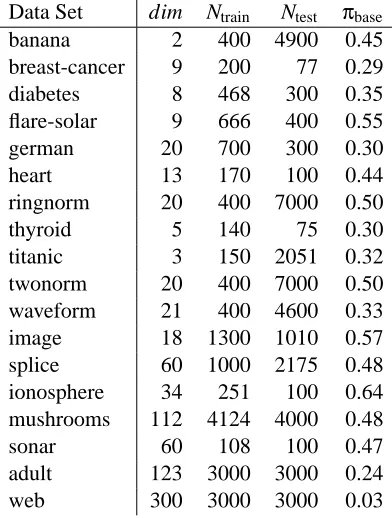
Data Set dim Ntrain Ntest πbase
banana 2 400 4900 0.45
breast-cancer 9 200 77 0.29
diabetes 8 468 300 0.35
flare-solar 9 666 400 0.55
german 20 700 300 0.30
heart 13 170 100 0.44
ringnorm 20 400 7000 0.50
thyroid 5 140 75 0.30
titanic 3 150 2051 0.32
twonorm 20 400 7000 0.50
waveform 21 400 4600 0.33
image 18 1300 1010 0.57
splice 60 1000 2175 0.48
ionosphere 34 251 100 0.64
mushrooms 112 4124 4000 0.48
sonar 60 108 100 0.47
adult 123 3000 3000 0.24
web 300 3000 3000 0.03
Table 1: Description of data sets. dim is the number of features, and Ntrainand Ntestare the numbers of training and test examples.πbaseis the proportion of positive examples (novelties) in the combined training and test data. Thus, the average (across permutations) nominal sample size m is(1−πbase)Ntrain.
raetsch/benchmarkand the last five data sets (Chang and Lin, 2001) are fromhttp://www.csie. ntu.edu.tw/˜cjlin/libsvmtools/datasets/.
Each data set consists of both positive and negative examples. Furthermore, each data set is replicated 100 times (except for image and splice, which are replicated 20 times), with each copy corresponding to a different random partitioning into training and test examples. All numerical results for a data set were obtained by averaging across all partitions. The negative examples from the training set were taken to form the nominal sample, and the positive training examples were not
used at all in the experiments. The data sets are summarized in Table 1. Here Ntrainand Ntestare the
sizes1of the training and test sets, respectively, whileπbaseis the proportion of positive examples in the combined training and test data. Thus, the average (across permutations) nominal sample size m is(1−πbase)Ntrain.
We emphasize that in these experiments we do not implement the empirical risk minimization (ERM) algorithm from Sec. 4. The reduction to Neyman-Pearson classification is general and can by applied in conjunction with any NP classification algorithm, whether that algorithm has associated performance guarantees or not. We here elect to apply the reduction using a plug-in kernel density estimate (KDE) classifier. ERM is computationally infeasible, and the bounds tend
to be too loose in practice to be effective. The KDE plug-in rule can be implemented efficiently, and there is a natural inductive counterpart for comparison, the thresholded KDE based on the nominal sample.
8.1 Experimental Setup
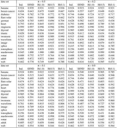
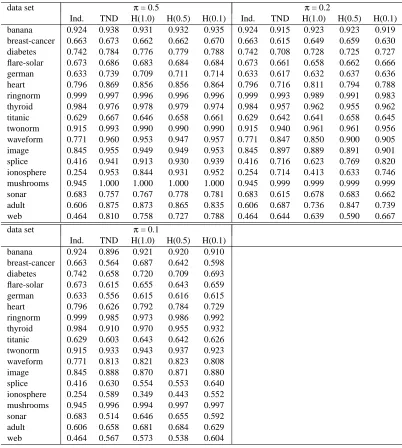
We evaluated our methodology in two learning paradigms, comparing five learning methods across
several values ofπ. The two learning paradigms are supervised and transductive. For
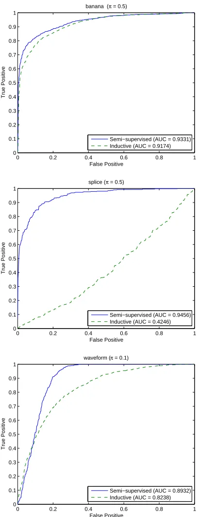
semi-supervised learning, the test data were divided into two halves. The first half was used as the contaminated, unlabeled data. The second half was used as an independent sample of contaminated data, not used in the learning stage, but only for evaluation of classifiers returned by each method. In particular, the second half of the test data was used to estimate the area under the ROC (AUC)
of each method. Here, the ROC is the one which views P0 as the null distribution and P1 as the
alternative. For transductive learning, the entire test set was treated as the unlabeled data, and was also used for evaluating the AUC.
The learning methods are the inductive approach, our proposed learning reduction, and three versions of the hybrid approach. The three hybrids correspond to pn=1.0, 0.5, and 0.1, in which a
uniform sample of size 100pn% of the unlabeled sample size is appended to the unlabeled data. We
emphasize that each algorithm was implemented in the same way in the two learning paradigms; the only differences are the size of the contaminated sample, and how they are evaluated.
We implemented the inductive novelty detector using a thresholded kernel density estimate (KDE) with Gaussian kernel, and SSND using a plug-in KDE classifier. To alleviate concerns that our inductive implementation is inadequate, we also tested the one-class support vector ma-chine (Sch¨olkopf et al., 2001) in several experimental settings, and found its performance to be very
similar. Letting kσ denote a Gaussian kernel with bandwidthσ, the inductive novelty detector at
density levelλis
f(x) =
1 if m1∑mi=1kσ0(x,xi)>λ
0 otherwise,
and the SSND classifier at density ratioλis
f(x) =
1 if(1
n∑
m+n
i=m+1kσX(x,xi))/( 1
m∑
m
i=1kσ0(x,xi))>λ
0 otherwise.
The hybrid method is implemented similarly. The ROCs of these methods are obtained by varying the level/thresholdλ.
For each class, a single kernel bandwidth parameter was employed, and optimized by maximiz-ing a cross-validation estimate of the AUC. Note that this ROC is different from the one used to
evaluate the methods (see above). In particular, it still views P0 as the null distribution, but now
the alternative distribution is taken to be the uniform distribution P2for the inductive detector (see Section 5; effectively we use a uniform random sample of size n in place of the unlabeled data),
PX for SSND, and the appropriate ˜PX for the hybrid methods (see Section 5). Thus, the test label
information was not used at any stage (prior to validation) by any of the methods.
We also compared the learning methods for several values ofπ. For semi-supervised learning,
we examinedπ=0.5,π=0.2,π=0.1, andπ=0.0. For transductive learning, we examinedπ=
0.5,π=0.2, and π=0.1. The case π=0.0 cannot be evaluated in the transductive paradigm