Application of machine learning techniques for detecting anomalies in communication networks

(1)

Application of Machine Learning

Techniques for Detecting Anomalies in

Communication Networks

by

Qingye Ding

M.Sc., New Jersey Institute of Technology, 2014 B.Sc., Northeast Agricultural University, 2012

Thesis Submitted in Partial Fulfillment of the Requirements for the Degree of

Master of Applied Science

in the

School of Engineering Science Faculty of Applied Science

c

Qingye Ding 2018

SIMON FRASER UNIVERSITY Summer 2018

Copyright in this work rests with the author. Please ensure that any reproduction or re-use is done in accordance with the relevant national copyright legislation.

(2)

Approval

Name: Qingye Ding

Degree: Master of Applied Science (Engineering Science) Title: Application of Machine Learning Techniques for

Detecting Anomalies in Communication Networks Examining Committee: Chair: Ivan V. Bajić

Professor Ljiljana Trajković Senior Supervisor Professor Parvaneh Saeedi Supervisor Associate Professor Qianping Gu Internal Examiner Professor

School of Computing Science

(3)

Abstract

Detecting, analyzing, and defending against cyber threats is an important topic in cyber security. Applying machine learning techniques to detect such threats has received consid-erable attention in research literature. Anomalies of Border Gateway Protocol (BGP) affect network operations and their detection is of interest to researchers and practitioners. In this Thesis, we describe main properties of the BGP and datasets that contain BGP records col-lected from various public and private domain repositories such as Réseaux IP Européens (RIPE) and BCNET.

With the advent of fast computing platforms, the neural network-based algorithms have proved useful in detecting BGP anomalies. We apply the Long Short-Term Memory machine learning technique for classification of known network anomalies. The models are trained and tested on various collected datasets. Various classification techniques and approaches are compared based on accuracy and F-Score.

Keywords: Border Gateway Protocol; routing anomalies; machine learning; classification algorithms; long short-term memory

(4)

Acknowledgements

I would like to express my sincere appreciation to my advisor Prof. Ljiljana Trajković for her great guidance with my research, for her patience, kindness, and immense knowledge.

I would also like to thank the rest of my committee: Prof. Ivan V. Bajić, Prof. Qianping Gu, and Prof. Parvaneh Saeedi, for their insightful comments and suggestions.

My thanks also go to my friends and colleagues in Communication Networks Laboratory at Simon Fraser University for their support and assist during my graduate study.

Finally, I would like to thank my family for supporting me spiritually throughout writing this Thesis. In particular, I am grateful to my husband for his wise counsel and sympathetic ear. You were always there for me.

(5)

List of Tables

Table 1.1 Sample of a BGP update message. IGP: Interior Gateway Protocol;

NLRI: Network layer reachability information. . . 3

Table 2.1 Examples of known BGP Internet worms. . . 17

Table 2.2 Internet anomalous events. . . 20

Table 2.3 Training and test datasets. . . 23

Table 3.1 List of features extracted from BGP update messages. . . 27

Table 3.2 Definition ofvolumeandAS-path features extracted from BGP update messages. . . 28

Table 3.3 Example of BGP features. . . 28

Table 4.1 Confusion matrix. . . 32

Table 4.2 The actions of the internal state corresponding to values of input and forget gates. . . 37

Table 5.1 Accuracy and F-Score using various classification models for unbal-anced datasets. . . 49

Table 5.2 Accuracy and F-Score using LSTM and SVM models for balanced datasets. . . 51

(8)

List of Figures

Figure 1.1 Illustration of the machine learning process. . . 4 Figure 1.2 Illustration of the 10-fold cross validation. The original training dataset

is partitioned into 10 folds. Each fold is used once as a validation set during the training phase. The final estimation result is the average number of the 10 validation results. . . 5 Figure 1.3 Procedure of data clustering with a feedback loop. The result of

clus-tering may affect feature extraction/selection and the computation of pattern proximity. . . 7 Figure 1.4 Illustration of hard clustering in a 2-dimensional space. The vertical

and horizontal axis represent two dimensions. Each data point in the original dataset (a) is clustered to a single cluster (b). Triangle and circle represent features of the dataset. . . 8 Figure 1.5 Shown is an example of fuzzy clustering in a 2-dimensional space.

The vertical and horizontal axis represent two dimensions. Each data point in the original dataset (a) may belong to multiple clusters (b). 9 Figure 1.6 Example of hierarchical clustering. The vertical axis represents the

similarity between clusters and the horizontal axis represents the combined clusters. Each data point in the original dataset (a) is considered as a single cluster (b). These clusters are merged based on their similarity. . . 10 Figure 1.7 Example of partitional clustering. The vertical and horizontal axis

represent two dimensions. Several centroid points are selected from the original dataset (a). The algorithm then calculates proximity of clusters (b). Centroid points and clusters are updated based on the proximity (right). . . 10 Figure 1.8 Example of a recurrent neural network (RNN). A node represents a

unit. An RNN is unrolled by expanding its computation graph to a directed acyclic graph. Shown is an expanded RNN at timest−1,t, andt+ 1. . . 13

(9)

Figure 2.1 Number of BGP announcements occurred between January 23, 2003 and January 28, 2003. The announcements occurred during Slammer anomaly are labeled as the “anomaly” class while others belong to the “regular” class. . . 18 Figure 2.2 Number of BGP announcements occurred between September 16,

2001 and September 21, 2001. The number of announcements issued during Nimda anomaly are labeled as the “anomaly” class while oth-ers belong to the “regular” class. . . 19 Figure 2.3 Number of BGP announcements issued from July 17, 2001 to July

22, 2001. The number of announcements occurred during Code Red I anomaly are labeled as the “anomaly” class while others belong to the “regular” class. . . 20 Figure 2.4 Number of BGP announcements occurred between December 18,

2001 and December 22, 2001. Shown is an example of BGP announce-ments occurred during regular traffic. The number of announceannounce-ments belong to the “regular” class. . . 21 Figure 2.5 BGP announcements occurred during the Slammer worm attack:

number of duplicate announcements (top) and number of EGP pack-ets (bottom). The red streams (light grey) are anomalous data points and the blue (dark grey) ones are regular data points. . . 24 Figure 2.6 BGP announcements occurred during the Slammer worm attack:

maximum AS-path length (top) and maximum AS-path edit dis-tance (bottom). The red streams (light grey) are anomalous data points and the blue (dark grey) ones are regular data points. . . 25

Figure 3.1 Distribution of the maximum AS-path length (top) and the max-imum edit distance (bottom) collected during the Slammer worm. Shown maximum AS-paths contains up to 24 ASes, and the paths change frequently. . . 29 Figure 3.2 Distribution of the number of BGP announcements (top) and

with-drawals (bottom) for the Code Red I worm. . . 30

Figure 4.1 Shown is an example of a simple RNN with an input layer, a hidden layer, and an output layer. The loss is calculated using the prediction value and the target value. . . 34 Figure 4.2 Repeating module for the LSTM neural network. Shown are the

in-put layer, LSTM layer with one LSTM cell, and outin-put layer. . . . 35 Figure 4.3 Architecture of the employed LSTM classifier. Shown are input layer

with 37 nodes, LSTM layer with 256 cells, the dropout layer with 50% dropout rate, and the output layer. . . 38

(10)

Figure 5.1 Illustration of the soft margin SVM [8]. Shown are correctly and incorrectly classified data points. Regular and anomalous data points are denoted by circles and stars, respectively. The circled points are support vectors. . . 41 Figure 5.2 Illustration of the role of a kernel function. Blue circles and yellow

stars are regular and anomalous data points, respectively. A nonlin-ear kernel function maps the input data points from input space to a higher dimensional feature space and calculates an optimal separat-ing hyperplane. Then the hyperplane is mapped back to input space and results in a nonlinear decision boundary. . . 42 Figure 5.3 An example of the Decision Tree used to detect a BGP anomaly.

The input data points are categorized based on the features shown in rectangles. The classification results are shown by ellipses that represent leaf nodes. . . 45 Figure 5.4 Neural network architecture of the ELM algorithm. Shown structure

consists of an input layer withd dimensions, a hidden layer with k hidden neurons, and an output layer withm output samples. . . 47

(11)

Chapter 1

Introduction

1.1

Overview of Border Gateway Protocol (BGP)

Border Gateway Protocol (BGP) [1] is a routing protocol that plays an essential role in for-warding Internet Protocol (IP) traffic between the source and the destination Autonomous Systems (ASes). An Autonomous System (AS) is a collection of BGP peers (neighbors) managed by a single administrative domain [2]. It consists of one or more networks that possess uniform routing policies while operating independently. Internet operations such as connectivity and data packet delivery are facilitated by various ASes.

The main function of BGP is to select the best routes between ASes based on network policies enforced by network administrators. Routing algorithms determine the route that a data packet takes while traversing the Internet. They exchange reachability information about possible destinations. BGP is an upgrade of the Exterior Gateway Protocol (EGP) [3]. It is an interdomain routing protocol used for routing packets in networks consisting of a large number of ASes. BGP version 4 allows Classless Interdomain Routing (CIDR), aggregation of routes, incremental additions, better filtering options, and it has the ability to set routing policies. BGP employs the Path Vector protocol, which is a modified version of the Distance Vector protocol [5]. It is a standard for the exchange of information among the Internet Service Providers (ISPs).

BGP relies on the Transport Control Protocol (TCP) to establish a connection (port 179) between the routers. A BGP router establishes a TCP connection with its peers that reside in different ASes. Because of their size, BGP routing tables are exchanged once between the peering routers when they first connect. BGP allows ASes to exchange reachability information with peering ASes to transmit information about the availability of routes within an AS. Based on the exchanged information and routing policies, it determines the most appropriate path to destination. Hence, BGP allows each subnet to announce its existence to the Internet and to publish its reachability information. Hence, all sub-networks are interconnected and are known to the Internet.

(12)

BGP is an incremental protocol that sends updates only if there are reachability or topology changes within the network. Afterwards, only updates regarding new prefixes or withdrawals of the existing prefixes are exchanged. BGP routers exchange four types of mes-sages: open, update, keep-alive, and notification [3]. After a transport protocol connection is established, the open message that contains basic information such as router identifier, BGP version, and the AS number is used to open a peering session. Once the open mes-sage is confirmed,update,keep-alive, andnotification messages are exchanged. BGP routers exchange known routing information using theupdate message after the BGP session is es-tablished and when there is a change of BGP routes in their routing tables. They advertise only one available route, withdraw multiple unavailable routes, or execute both simultane-ously. Network Layer Reachability Information (NLRI) field of theupdatemessage contains attributes of all paths that apply to the destination. TheUpdate message contains informa-tion of the relainforma-tionships among various ASes. It may be used to detect network anomalies and prevent routing loops. The Minimal Route Advertisement Interval (MRAI) limits the minimum time interval between two update messages that are sent to the same destination. The default MRAI value is 30 s in practice [4]. Instead of using transport protocol to deter-mine if peers are reachable, BGP routers frequently exchangeskeep-alivemessages between peers during inactivity periods to ensure that the connections do not expire the hold time, which is usually 90 seconds. The maximum interval betweenkeep-alivemessages is typically one third of thehold timeinterval. Thenotificationmessage closes a peering session if there is a disagreement in the configuration parameters.

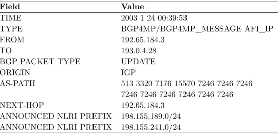
A sample of a BGP update message is shown in Table 1.1. The Origin attribute is generated by the AS that originates the routing information. It is a mandatory attribute and will be propagated to other BGP speakers that are used to advertise the routing information. The AS-path attribute in the BGP update message indicates the path that a BGP packet traverses among AS peers. Only when a BGP speaker propagates a route to another BGP speaker located within the same AS, the AS-path attribute will not be modified. The AS-path attribute enables BGP to route packets via the best path. The next-hop attribute defines the IP address of the next hop to the destination. NLRI announcements share a list of IP address prefixes.

Propagation of the BGP routing information is susceptible to various anomalous events such as worms, malicious attacks, power outages, blackouts, and misconfigurations of BGP routers. BGP anomalies are caused by changes in network topologies, updated AS policies, or router misconfigurations. They affect the Internet servers and hosts and are manifested by anomalous traffic behavior. Anomalous events in communication networks cause traffic behavior to deviate from its usual profile. These events may spread false routing information throughout the Internet by either dropping packets or directing traffic through unauthorized ASes and, hence, risking eavesdropping. Large-scale power outages may affect ISPs due to unreliable power backup. They could also cause network equipment failures leaving affected

(13)

Table 1.1: Sample of a BGP update message. IGP: Interior Gateway Protocol; NLRI: Net-work layer reachability information.

Field Value

TIME 2003 1 24 00:39:53

TYPE BGP4MP/BGP4MP_MESSAGE AFI_IP

FROM 192.65.184.3

TO 193.0.4.28

BGP PACKET TYPE UPDATE

ORIGIN IGP

AS-PATH 513 3320 7176 15570 7246 7246 7246 7246 7246 7246 7246 7246 7246

NEXT-HOP 192.65.184.3

ANNOUNCED NLRI PREFIX 198.155.189.0/24 ANNOUNCED NLRI PREFIX 198.155.241.0/24

networks isolated and their service disrupted. Configuration errors in BGP routers also induce anomalous routing behavior. Routing table leak and prefix hijack [6] events are examples of BGP configuration errors that may lead to large-scale disconnections in the Internet. A routing table leak occurs when an AS (such as an ISP) announces a prefix from its Route Information Base (RIB) that violates previously agreed upon routing policy. A prefix hijack is the consequence of an AS originating a prefix that it does not own.

1.2

Machine Learning Techniques

Machine learning is a subfield of artificial intelligence, which is closely related to statistics and various interdisciplinary fields, such as neocognitron in biology [7], cognitive science, control theory, and information theory [8]. Unlike traditional computing techniques, machine learning enables computers to build models and make decisions based on input datasets. Machine learning was defined [9] as a computer program that could learn from experiences with respect to classes of objectives and performance metrics, as long as they improve the experience.

The concept of machine learning was introduced in Alan Touring’s paper “Computing Machinery and Intelligence” [10]. Machine learning gained more attention after he brought up the research question “Can machines think?” in 1950. Since 1990s, machine learning flourished and became well known. In 2006, Geoffrey Hinton introduced the deep learning and proved that machines are able to distinguish objects and texts in images and videos [11]. Machine learning is able to analyze complex and large volume of data, which makes it cru-cial in various areas. For example, image recognition technology allows surveillance cameras to detect faces; speech recognition translates spoken words into texts while recommender systems suggest commodities based on user preferences. Machine learning techniques have

(14)

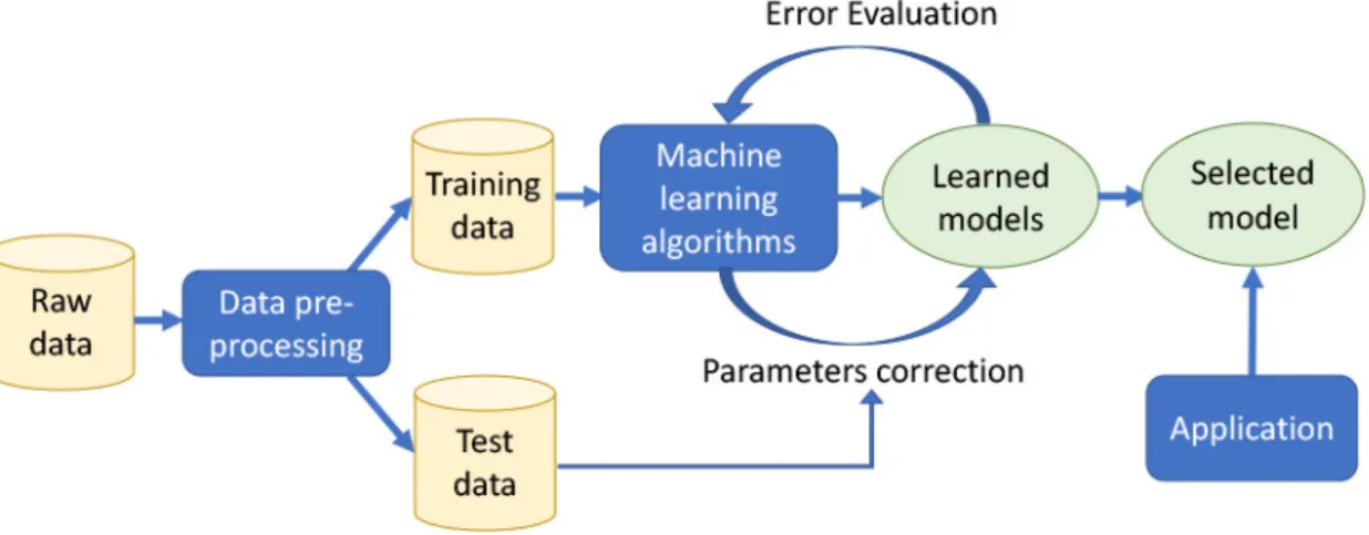
also been employed to develop models for detecting anomalies and designing BGP anomaly detection systems [12]. They are the most common approaches for classifying BGP anoma-lies. A typical goal of machine learning applications is to map input instances to an output value. An illustration of the machine learning process is shown in Fig. 1.1.

Figure 1.1: Illustration of the machine learning process.

1.2.1 Machine Learning Process

Raw data typically contain missing values and redundant information and, thus, they need to be parsed, cleaned, pre-processed, and transformed into a proper form. The data is then divided into training and test datasets. In the training phase, the machine learning algo-rithms are applied to the training data to create candidate models. Models “observe” and learn from the training dataset. However, a model may be biased due to the limited number of data points that the model has observed. In order to avoid such biased observations, the validation phase is introduced to estimate the quality of the model based on classification accuracy, recall, precision, or F-Score. Hyperparameters of the model are tuned based on the validation results to improve the existing model.

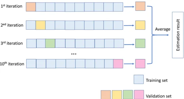
K-fold cross-validation is commonly used in machine learning tasks [13]. The advantage of using k-fold cross validation is that the training dataset is fully used for both training and validating, and each subset is used for validation only once. In the k-fold cross-validation, the original training dataset is randomly partitioned into k equal-sized subsets. For example, for a 10-fold validation set, machine first partitions the training dataset into 10 subsets and then randomly shuffles them. Nine subsets are trained and one is left out as a validation set to estimate the quality of the model. This process repeats until all subsets have been used as both training and validation sets and have returned 10 estimation results. The average

(15)

number of the 10 results is the final estimation of the model. An illustration of a 10-fold cross validation is shown in Fig. 1.2.

Figure 1.2: Illustration of the 10-fold cross validation. The original training dataset is par-titioned into 10 folds. Each fold is used once as a validation set during the training phase. The final estimation result is the average number of the 10 validation results.

The validation phase is also used to prevent underfitting and overfitting. If the training and validation accuracy are both low, the model is underfitting, and it is not suitable for training datasets. The solution may be to use alternative machine learning algorithms or increase the number of iterations. In practice, underfitting is easy to detect while overfitting is rather challenging. If the training accuracy is high while the validation accuracy is very low, the model is probably overfitting, which implies that the model learns too well details including noise information in the training dataset and it may fail to reliably fit future observations [14]. The overfitting model learns the noise data as the useful information and captures details of the dataset. However, the capture does not suitable for new dataset and negatively impacts the generality of the model. Overfitting is more likely to happen when training nonparametric (the complexity of the model increases with the number of the training data) or nonlinear models that have distribution-free structures. Therefore, machine learning models for nonparametric datasets may use techniques to constrain the information that the model may learn. For example, a Long Short-Term Memory nonparametric model addresses overfitting by using dropout technique [15] by removing a certain portion of information that it has learned. The validation phase repeats until the validation accuracy becomes constant and is within a certain threshold. In most cases, the validation error is larger than the training error. Empirically, the training and validation sets within the

(16)

original training dataset are split in proportions 7:3 or 8:2. How to split the dataset mainly depends on the total number of data samples and properties of the training model. For example, in case of a model that needs a large number of data to train, the validation subset may be reduced to optimize the performance.

After the validation phase, test data are used to evaluate the developed models. The difference between validation and test sets is that the validation set is partitioned from the training set while the test set is only released when the training and validation phases are completed. The test set should not be learned beforehand. Otherwise, the learning is invalid. Generally the test dataset contains data samples with various classes that the model would encounter the reality. The model is then applied to the real-world data after the procedure of training, validation, and test phases.

There are various types of machine learning algorithms. They may be grouped as un-supervised or un-supervised learning based on their characteristics. A key distinction between unsupervised and supervised learning techniques is the target (label) [8]. For unsupervised learning, the task is to find the relationships among various unlabeled inputs. For supervised learning, every training input has a corresponding target (label) and the machine provides labels for new inputs after sufficient training.

1.2.2 Unsupervised Learning

Unsupervised learning aims to learn a function that represents the underlying structure from unlabeled input data by reducing amount or dimension of input datasets and tuning a set of parameters. The main motivation for using unsupervised learning is the labeled data is difficult to obtain, limited in quantity, and may contain errors. Unsupervised machine learning models have been used to detect anomalies in networks with non-stationary traf-fic [16]. The one-class neighbor machines [17] and recursive kernel-based [18] online anomaly detection algorithms are effective methods for detecting anomalous network traffic [19]. An online algorithm does not need to “observe” the entire input data and it may provide par-tial solutions at each iteration. In contrast, all offline algorithm requires apriori to have the entire data in order to produce the ultimate solution of the problem.

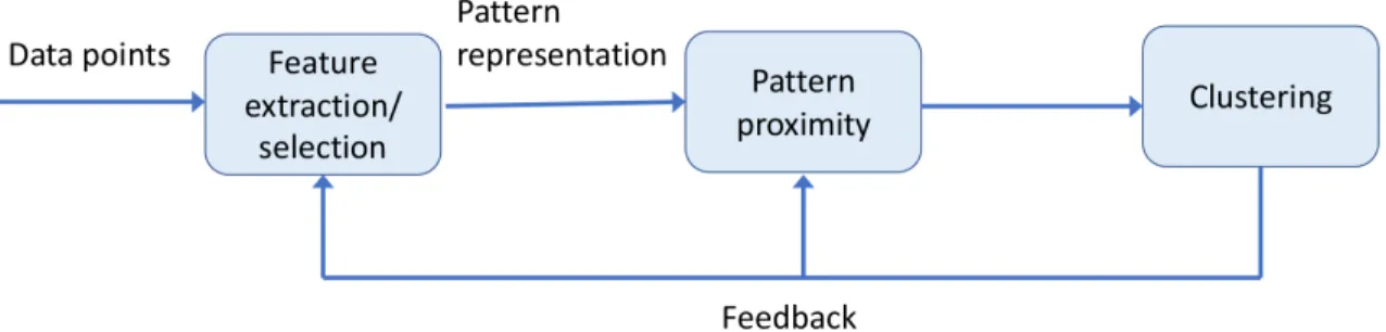
Data clustering is a commonly-used technique of unsupervised learning. Data points are grouped together based on their closeness in a suitable feature space. The goal of data clustering is to assign data points with similar traits into the same group. The procedure of data clustering typically includes feature extraction/selection, pattern representation, pattern proximity, and clustering. The procedure is illustrated in Fig. 1.3. Feature extraction technique transforms the original input data and extracts desired features. Feature selection is the process where the system selects the most effective features from the original dataset. These techniques may be used in clustering to obtain the most suitable feature sets. Pattern representation refers to the information extracted or selected from the original dataset such

(17)

Figure 1.3: Procedure of data clustering with a feedback loop. The result of clustering may affect feature extraction/selection and the computation of pattern proximity.

as the number of classes, types, and the number of available patterns. Pattern proximity basically forms the elements in a group when they are placed close to each other.

Distance functions are used to measure distances between pairs of patterns. The mea-surement of distance should be carefully selected because the feature types and scales vary in a dataset. The Euclidean distance is the most commonly used metric to evaluate the proximity of patterns. It is well suited for datasets with isolated clusters. The Euclidean distance [20] between two data points is the length of the straight line between them. It is calculated as: distEuc(xi, xj) = q (Pd k=1(xi,k−xj,k)2) =||xi−xj||2, (1.1)

wherexi,xj, andxk are data points in a d-dimensional feature space, wherexi has coordi-nates xik,· · ·, xid and xj has coordinatesxjk,· · · , xjd. Euclidean distance is a special case that is only suitable for data points in two or three dimensional space. A general form of Euclidean distance is the Minkowski distance [21]. For higher dimensional feature space d, Minkowski metric uses theLp norm that is calculated as:

distp(xi, xj) = p q (Pd k=1(xi,k−xj,k)p) =||xi−xj||p, (1.2)

Another well-known metric is Cosine distance. It measures the divergence between a pair of data points using the cosine of the angle between their locations. The Cosine distance is well suited for high-dimensional data. Thus, it is widely used in data mining for tasks with large datasets such as identifying plagiarism. The Cosine distance is calculated as:

distcos(xi, xj) = 1−cos(x[i, xj) = 1− Pd k=1(xik·xjk) q Pd k=1(xik) 2 q Pd k=1(xjk) 2 (1.3)

(18)

After the pattern proximity is identified, clustering algorithms are used. It is the key of the data clustering procedure. Clustering techniques may be divided into several categories.

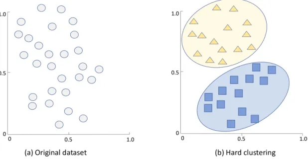
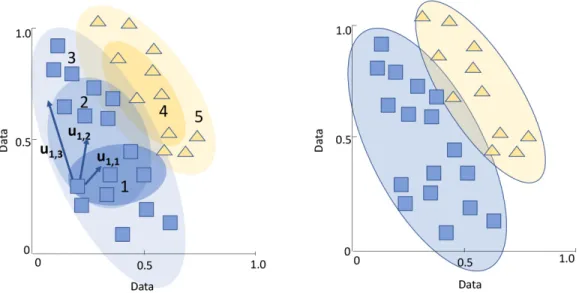
Hard vs. fuzzy clustering techniques: Clustering techiniques may be categorized as hard or fuzzy (soft) based on the clustering output. A hard clustering algorithm assigns each data point to a distinct cluster and each data point may only belong to one cluster. Instead of assigning data points to distinct clusters, a fuzzy clustering (also called soft clustering) may assign each data point to multiple clusters. Membership grade is used in the soft clustering to maintain a list of cluster nodes without inappropriate duplications. The list continuously changes during the clustering procedure. Based on the membership list, soft clustering algorithms assign each data point a likelihood to indicate the probability of a data to be allocated in different clusters. An examples of hard clustering method is shown in Fig. 1.4. An illustration of fuzzy clustering is shown in Fig. 1.5. Each data point in the original dataset is assigned a membership degree for each cluster that it may be allocated. For instance, data point 1 (a) has membership degreesu1,1,u1,2, andu1,3 corresponding to

its potential clusters 1, 2, and 3, respectively. The final clustering result (b) is generated based on membership degrees of all data points.

Figure 1.4: Illustration of hard clustering in a 2-dimensional space. The vertical and hori-zontal axis represent two dimensions. Each data point in the original dataset (a) is clustered to a single cluster (b). Triangle and circle represent features of the dataset.

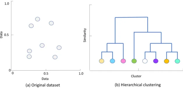
Hierarchical vs. partitional clustering techniques: The goal of hierarchical clustering is to group data into a hierarchy or a tree of clusters. Hierarchical clustering algorithms ini-tially assume that each data point is a cluster. The algorithms then compute the proximity (similarity between clusters) and combine pairs of the most similar clusters. The procedure

(19)

Figure 1.5: Shown is an example of fuzzy clustering in a 2-dimensional space. The vertical and horizontal axis represent two dimensions. Each data point in the original dataset (a) may belong to multiple clusters (b).

continues until reaching a pre-defined number of clusters. Unlike hierarchical methods, par-titional clustering techniques do not initialize each point as a cluster. Instead, they randomly select some of the points as centers of clusters. The center point is called the centroid. Each data point is randomly assigned to a cluster. The algorithms then compute the proximity between each center and data point, update the centroid, and re-assign data points to the cluster with the most similar centroid. The procedure repeats until the number of clusters reaches a pre-defined threshold. Examples of hierarchical and partitional clustering methods are shown in Fig. 1.6 and Fig. 1.7.

Among clustering algorithms, k-means, which belongs to the partitional clustering method, has been widely used in machine learning tasks such as Natural Language Programming [8]. The number of clusters is decided apriori based on mixture models, a hierarchical clustering algorithm, or a neural network-based method such as the Kohonen map [22].

The ultimate goal of clustering is to find the most appropriate partitioning that fits the underlying data. To evaluate the performance of clustering algorithms, various clustering validation techniques have been used [23]. They may be classified into three approaches: external measurement, internal measurement, and relative criteria. External measurement evaluates the clustering results based on pre-specified ground truth that is not contained in the dataset such as structures of underlying dataset and labels. Well known metrics of external measurement are F-Score, purity, and entropy. Internal measurement validates the

(20)

Figure 1.6: Example of hierarchical clustering. The vertical axis represents the similarity between clusters and the horizontal axis represents the combined clusters. Each data point in the original dataset (a) is considered as a single cluster (b). These clusters are merged based on their similarity.

Figure 1.7: Example of partitional clustering. The vertical and horizontal axis represent two dimensions. Several centroid points are selected from the original dataset (a). The algorithm then calculates proximity of clusters (b). Centroid points and clusters are updated based on the proximity (right).

(21)

properties of created clusters in order to determine if the data points are well partitioned. These properties may be the distance between clusters, intra-cluster distance, or distances among certain points that belong to different clusters. Metrics of internal measurement [24] include Bayesian information criterion, Calinski-Harabasz index, and Dunn index. The ma-jor drawback of external and internal measurement is high computational demands. Thus, relative criteria [25] is introduced to avoid statistical tests. The approach of relative cri-teria is to compare a set of defined cluster schemes and select the one that best fits the pre-specified criterion.

1.2.3 Supervised Learning

Supervised learning encompasses most of the traditional types of machine learning. Unlike unsupervised learning, supervised learning obtains information and builds predictions from observed input data. In supervised learning, a labeled dataset with a specific predictive goal is given, where each observation from the dataset associates with a label corresponding to the predictive goal. A learning algorithm or classifier trains data based on the observation to predict the label for new events [8]. An example is detecting email spam, where supervised learning aims to accurately detect whether a newly received email is spam by training a large number of past emails labeled as either spam or not spam [26].

We denote a labeled training dataset as:

S= (X1, Y1),(X2, Y2),· · · ,(Xn, Yn), Xi ∈Ω, Yi ∈ {−1,1}, (1.4) where the i’th observation Xi is in a feature space Ω. We use m features/dimensions in this Thesis. Hence, X ∈ _Rm _{and Ω =}

Rm. The label of Xi is denoted by Yi. For binary classification problems, we use two labels: -1 for regular and 1 for anomaly. The goal of supervised learning is to train a function that maps a new observation X ∈ Ω to a label Y ∈ {−1,1}:

f(X;θ)7→ {−1,1}, (1.5) where vector θ represents a set of parameters optimized by the classification algorithm to enhance the accuracy of the classifier.

Most applications employ features for classification tasks. If the function is very simple, such as a linear function f(X;θ) = θ>X, the classification results may only fulfill simple tasks by using few parameters. Furthermore, if the training dataset is relatively small, it is difficult to train a complex function with many parameters due to the risk of overfitting.

Supervised learning is employed for anomaly classification when the input data are la-beled based on various categories. Well-known supervised learning algorithms include Long Short-Term Memory (LSTM) [27], [28], Support Vector Machine (SVM) [8], [29], Hidden Markov Model (HMM) [8], Naïve Bayes [30], Decision Tree [31], and Extreme Learning Machine (ELM) [32], [33]. The SVM algorithms often achieve better performance compared

(22)

to other machine learning algorithms albeit with high computational complexity. LSTM is trained using gradient-based learning algorithms implemented as a recurrent neural network. It outperforms other sequence learning algorithms because of its ability to learn long-term dependencies from past experiences. No single learning algorithm performs the best for all given classification tasks [34]. Hence, an appropriate algorithm needs to be selected by eval-uating its performance based on various parameters. Statistical methods, data mining, and machine learning have been employed to evaluate and compare various algorithms [35], [36].

1.3

Recurrent Neural Network

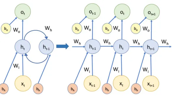
Recurrent Neural Networks (RNNs) are artificial neural network models that enable net-works to deal with sequence recognition, pattern classification, and temporal prediction tasks with sequential inputs and outputs by performing temporal processing and sequence learning [37]. Basic RNNs consist of neuron-like nodes that directly connects to any other node. An RNN contains three types of elements: input node, hidden state, and output node. The input node receives input data from various sources and passes the information to the hidden state. The hidden state may be considered as the memory of the network. The en-tire memory calculated from previous time steps is reserved in the current hidden state. In practice, a traditional RNN may only capture information from limited previous time steps. The output node shows the prediction result that is calculated based on the hidden state. Across the entire learning procedure, a RNN shares the same parameters such as weights for input node, hidden state, and output node, respectively. It implies that the network is performing the same at each time step with different inputs, which reduces the total num-ber of parameters that need to be learned. Although RNNs perform the same computation for each input element, various values of hidden states lead to different outcomes of the outputs. A typical architecture of an RNN is shown in Fig. 1.8.

At time t, the hidden state ht is calculated based on the input xt at the current time and the previous hidden state ht−1:

ht=f(Wixt+Whht−1+bh), (1.6)

where f denotes an activation function that updates at each time step t = 1, 2,· · ·. The function is typically a nonlinear function such astanhor Rectified Linear Unit (ReLU).Wi is the matrix of conventional weights between the input and the hidden layers while Wh is the matrix of recurrent weights between the hidden layers at adjacent time steps. The vectorbh is a bias parameter that is added to the hidden layers. The bias allows the hidden layer to generalize beyond the original dataset.

The output at time tis calculated as:

(23)

Figure 1.8: Example of a recurrent neural network (RNN). A node represents a unit. An RNN is unrolled by expanding its computation graph to a directed acyclic graph. Shown is an expanded RNN at times t−1,t, andt+ 1.

whereWodenotes the matrix of conventional weights between the hidden and output layers. The bias parameter is denoted by bo.

One of the most successful RNN architectures for sequence learning tasks is Long Short-Term Memory (LSTM) [28]. It introduces the memory cell which replaces traditional nodes in the hidden layer. The memory cells enable neural networks to overcome the problem of vanishing gradients that was encountered by earlier RNNs. Another successful RNN is Bidirectional Recurrent Neural Network (BRNN) [38]. Unlike the traditional RNNs that only calculate outputs based on the past memory, BRNN involves both the past and the future information to predict the output sequence. BRNN has been proved to be well-suited for sequence labeling tasks in natural language processing.

1.4

Motivation

The Internet is a critical asset of information and communication technology. Border Gate-way Protocol (BGP) plays an essential role in routing data between Autonomous Systems (ASes) where an AS is a collection of BGP peers administrated by a single administrative domain [39]. The main function of BGP is to select the best routes between ASes based on routing algorithms and network policies enforced by network administrators. BGP anomalies may be caused by changes in network topologies, updated AS policies, or router misconfig-urations. BGP anomalies affect Internet servers and hosts and are manifested by anomalous

(24)

traffic behavior. Hence, detecting such network anomalies is of great interest to researchers and practitioners.

1.5

Related Work

Detailed comparison of various network intrusion techniques has been reported in the litera-ture [40]. Demands for Internet services have been steadily increasing and anomalous events and their effects have dire economic consequences. Determining the anomalous events and their causes is an important step in assessing loss of data by anomalous routing. Hence, it is important to classify these anomalous events and prevent their effects on BGP.

Anomaly detection techniques have been applied in communication networks [19]. These techniques are employed to detect BGP anomalies such as intrusion attacks, worms, and distributed denial of service attacks (DDoS) [41], [42] that frequently affect the Internet and its applications. BGP data have been analyzed to identify anomalous events and design tools that have been used in anomaly predictions [42–47]. Network anomalies are detected by analyzing collected traffic data and generating various classification models. A variety of techniques have been proposed to detect BGP anomalies.

Early approaches include developing traffic models using statistical signal processing techniques where a baseline profile of network regular operation is developed based on a parametric model of traffic behavior and a large collection of traffic samples to account for regular (anomaly-free) cases [43]. Anomalies may then be detected as sudden changes in the mean values of variables describing the baseline model. However, it is infeasible to acquire datasets that include all possible cases. In a network with quasi-stationary traffic, statistical signal processing methods have been employed to detect anomalies as correlated abrupt changes in network traffic [44].

The main focus of other approaches also proposed in the past is developing models for classification of anomalies. The accuracy of a classifier depends on the extracted features, combination of selected features, and underlying models. Recent research reports describe a number of applicable classification techniques [45–47]. One of the most common approaches is based on a statistical pattern recognition model implemented as an anomaly classifier and a detector [45]. Its main disadvantage is the difficulty in estimating distributions of higher di-mensions. For example, a Bayesian detection algorithm was designed to identify unexpected route mis-configurations as statistical anomalies [46]. An instance-learning framework em-ployed wavelets to systematically identify anomalous BGP route advertisements [47]. Other proposed techniques are rule-based methods that have been employed for detecting BGP anomalies. An example is the Internet Routing Forensics (IRF) that was applied to classify anomaly events [48]. However, rule-based techniques are not adaptable learning mecha-nisms. They are slow, have high degree of computational complexity, and require a priority knowledge of network conditions.

(25)

Recent trends in designing BGP anomaly detection systems more frequently rely on machine learning techniques. Known classifiers are tested for their ability to reliably detect network anomalies in datasets that include known BGP anomalies. A survey of various meth-ods, systems, and tools used for detecting network anomalies reviews a variety of existing approaches [40]. The authors have examined recent techniques to detect network anoma-lies and discussed detection strategy and employed datasets, including performance metrics for evaluating detection method and description of various datasets and their taxonomy. They also identified issues and challenges in developing new anomaly detection methods and systems.

Various machine learning techniques to detect cyber threats have been reported in the literature. One-class SVM classifier with a modified kernel function was employed [49] to detect anomalies in IP records. However, unlike the approach in our studies, the classifier is unable to indicate the specific type of anomalies. Stacked LSTM networks [50] with sev-eral fully connected LSTM layers have been used for anomaly detection in time series. The method was applied to detect anomalous regions for medical electrocardiograms, space shut-tle Marotta’s valve time series , power demand, and engine sensors that measure dependent variables such as temperature and torque. The analyzed data contain both long-term and short-term temporal dependencies. Another example is the multi-scale LSTM [51] that was used to detect BGP anomalies using accuracy as a performance measure. In the preprocess-ing phase, data were compressed uspreprocess-ing various time scales. An optimal size of the slidpreprocess-ing window was then used to determine time scale in order to achieve the best performance of the classifier. Multiple HMM classifiers [52] were employed to detect Hypertext Trans-fer Protocol (HTTP) payload-based anomalies for various Web applications. Authors first treated payload as a sequence of bytes and then extracted features using a sliding window to reduce the computational complexity. HMM classifiers were then combined to classify network intrusions. It was shown [53] that the Naïve Bayes classifier performs well for cate-gorizing the Internet traffic emanating from various applications. Weighted ELM [54] deals with unbalanced data by assigning relatively larger weights to the input data arising from a minority class. Signature-based and statistics-based detection methods also have been proposed [55].

1.6

Research Contribution

In this Thesis, we consider BGP update messages because they contain the information about the protocol status and configurations. BGP update messages are extracted from the collected data during the time periods when the Internet experienced known anomalies. However, redundancies in the collected data may affect the performance of classification methods. Feature extractions are used to select a subset of features from the original feature space and, thus, reduce redundancy among features and improve the classification accuracy.

(26)

Various methods for feature extraction such as principal component analysis project the original data points onto a lower dimensional space. However, features transformed by feature extraction lose their original physical meaning. We extractAS-pathandvolumeBGP features based on the attributes of BGP update messages. We compare the performance of anomalies prediction use both unbalanced and balanced datasets.

We view anomaly detection as a classification problem of assigning an “anomaly” or “regular” label to a data point. We apply Long Short-Term Memory machine learning techniques to develop classification models for detecting BGP anomalies. These models are trained and tested using various datasets that consist extracted features. They are also used to evaluate the effectiveness of the extracted features. We improve classification results emanating from our previous studies [12,57,58] by carefully processing the considered datasets and selecting better parameters.

1.7

Organization of the Thesis

The Thesis is organized as follows: We first briefly describe BGP, the effect of network anomalies and approaches for their detection. In Chapter 2, we provide details of vari-ous BGP anomalies that have been considered in this Thesis as well as the description of datasets and the data processing. Various approaches to extract features from BGP up-date messages are described in Chapter 3. Performance metrics and the Long Short-Term Memory algorithm are introduced in Chapter 4. We introduce various classification algo-rithms and compare their classification results with the LSTM algorithm in Chapter 5. The challenges of detecting BGP anomalies as well as advantages and shortcomings of various classification algorithms are offered in Chapter 6. We describe the future work and conclude in Chapter 7. The list of references is provided in the Reference section.

(27)

Chapter 2

Border Gateway Protocol Datasets

2.1

Examples of BGP Anomalies

Anomalous events considered in this Chapter are worms. They are manifested by sharp and sustained increases in the number of announcement or withdrawal messages exchanged by BGP routers.VolumeandAS-pathfeatures are collected over one-minute time intervals dur-ing five-day periods for well known anomalous Internet events. While the available datasets contain data over much longer periods of time, we have selected for our analysis a five-day period to minimize storage and computational requirements. Furthermore, selecting longer periods of regular data would make datasets ever more unbalanced. Several methods that we surveyed offer better performance when dealing with balanced datasets. Details includ-ing dates of the events, remote route collectors (RRC) that acquired data usinclud-ing Routinclud-ing Information Service (RIS), and observed peers are given in Table 2.1. For example, Slam-mer event occurred on January 25, 2003 and lasted almost 16 hours. Hence, BGP update messages collected between January 23, 2003 and January 27, 2003 are selected as samples for feature extraction.

Table 2.1: Examples of known BGP Internet worms.

Dataset Class Date Duration

Beginning of the event End of the event (min) Slammer Anomaly 25.01.2003 at 5:31 GMT 25.01.2003 at 19:59 GMT 869 Nimda Anomaly 18.09.2001 at 13:19 GMT 20.09.2001 at 23:59 GMT 3,521 Code Red I Anomaly 19.07.2001 at 13:20 GMT 19.07.2001 at 23:19 GMT 600

Records of three BGP anomalies and regular RIPE traffic are shown in Fig. 2.1–Fig. 2.4. The effect of Slammer worm onvolumeandAS-pathfeatures is shown in Fig. 2.5 and Fig. 2.6. We consider Slammer [59], Nimda [60], and Code Red I [61] BGP anomalous events, other Internet anomalies are also listed in table 2.2.

Slammer [59]: The Structured Query Language (SQL) Slammer worm attacked Mi-crosoft SQL servers on January 25, 2003 [59]. MiMi-crosoft SQL servers were infected through

(28)

Figure 2.1: Number of BGP announcements occurred between January 23, 2003 and Jan-uary 28, 2003. The announcements occurred during Slammer anomaly are labeled as the “anomaly” class while others belong to the “regular” class.

a small piece of code that generated IP addresses at random. Furthermore, code replicated itself by infecting new machines through randomly generated targets. If the destination IP address was a Microsoft SQL server or a user’s PC with the Microsoft SQL Server Data Engine (MSDE) installed, the server became infected and began infecting other servers. The number of infected machines doubled approximately every nine seconds. As a result, the update messages consumed most of the routers’ bandwidth, which in turn slowed down the routers and, in some cases, caused the routers to crash. Single infected machines have re-ported additional traffic of 50 Mbps [62] as a consequence of increased generation of update messages.

Nimda [60]: The Nimda worm [60] exploited vulnerabilities in the Microsoft Internet Information Services (IIS) web servers for the Internet Explorer 5 on September 18, 2001. It propagated fast through email messages, web browsers, and file systems. The worm propagated by sending an infected attachment that was automatically downloaded after viewing the email messages. A user could also download it from the website or access an

(29)

Figure 2.2: Number of BGP announcements occurred between September 16, 2001 and September 21, 2001. The number of announcements issued during Nimda anomaly are labeled as the “anomaly” class while others belong to the “regular” class.

infected file through the network. The worm modified the content of the web document file in the infected hosts and copied itself in local host directories.

Code Red I [61]: Although the Code Red I worm attacked Microsoft IIS web servers earlier, the peak of infected computers was observed on July 19, 2001. The worm affected approximately half a million IP addresses a day. It took advantage of vulnerability in the Internet Information Services (IIS) indexing software. The worm replicated itself by exploit-ing weakness of the IIS servers and, unlike the Slammer worm, Code Red I searched for vulnerable servers to infect. It triggered a buffer overflow in the infected hosts by writing to the buffers without checking their limits. Rate of infection was doubling every 37 minutes.

Panix domain hijack: Panix, the oldest commercial ISP in New York state, was hijacked on January 22, 2006. Its services were unreachable from the greater part of the Internet. Con Edison (AS 27506) advertised routes that it did not own at the time. Panix was previously a customer of Con Edison, which was once authorized to offer advertised routes. Even though AS 27506 originated improper routes, major downstream ISPs did not properly configure filters and propagated those routes, leading to excess number of update messages.

(30)

Figure 2.3: Number of BGP announcements issued from July 17, 2001 to July 22, 2001. The number of announcements occurred during Code Red I anomaly are labeled as the “anomaly” class while others belong to the “regular” class.

Table 2.2: Internet anomalous events.

Event Date RRC Peers

Panix domain hijack Jan. 2006 Route Views AS 12956, AS 6762, AS 6939, AS 3549

AS 3356/AS 714 de-peering Oct. 2005 RIS 01 AS 13237, AS 8342, AS 5511, AS16034

Moscow power blackout May 2005 RIS 05 AS 1853, AS 12793, AS 13237 AS 9121 routing table leak Dec. 2004 RIS 05 AS 1853, AS 12793, AS 13237 AS-path error Oct. 2001 RIS 03 AS 3257, AS 3333, AS 6762,

AS 9057

AS 3561 improper filtering Apr. 2001 RIS 03 AS 3257, AS 3333, AS 286

De-Peering: The AS 3356/AS 714 De-Peering event occurred on October 5, 2005. Even though the Level 3 Communications (AS 3356) notified the Cogent Communications (AS 714) two months in advance of de-peering, the event created reachability problems for many Internet locations. Mostly affected were single-homed customers of Cogent (approximately

(31)

Figure 2.4: Number of BGP announcements occurred between December 18, 2001 and De-cember 22, 2001. Shown is an example of BGP announcements occurred during regular traffic. The number of announcements belong to the “regular” class.

2,300 prefixes) and Level 3 Communications (approximately 5,000 prefixes). De-Peering resulted in partitioning of approximately 4 % of prefixes in the global routing table.

Moscow power blackout: The blackout occurred on May 25, 2005 and lasted several hours. The Moscow Internet exchange was shut down during the power outage. Routing instabilities were observed due to loss of connectivity of several ISPs peering at this exchange. This effect was apparent at the RIS remote route collector in Vienna (rrc05) through a surge in announcement messages arriving from peer AS 12793.

AS 9121 routing table leak: It occurred on December 24, 2004 when AS 9121 announced to peers that it could be used to reach almost 70% of all prefixes (over 106,000). As a consequence, numerous networks had either misdirected or lost their traffic. The AS 9121 began announcing prefixes to peers around 9:20 GMT and the event lasted until shortly after 10:00 GMT. It continued to announce bad prefixes throughout the day. The announcement rate reached the second peak at 19:47 GMT.

AS 3561 improper filtering: This was a BGP mis-configuration error that occurred on April 6, 2001. AS 3561 allowed improper route announcements from its downstream

(32)

cus-tomers, which created connectivity disruptions. Surge of announcement messages originating from peer AS 3257 was observed at the RIS rrc03.

AS-path error: The AS-path error occurred on October 7, 2001. It was caused by an abnormal AS-path (AS 3300, AS 64603, AS 2008) that contained private AS 64603 that should not have been included in the path. At the time, AS 3300 and AS 2008 belonged to INFONET Europe and INFONET USA, respectively. The path was distributed to the network via mis-configured routers and caused the leak of the private AS numbers.

2.2

Analyzed BGP Datasets

The Internet routing data used in this Thesis to detect BGP anomalies is acquired from projects that provide valuable information to networking research: the Route Views project [63] at the University of Oregon, USA and the Routing Information Service (RIS) project initiated in 2001 by the Réseaux IP Européens (RIPE) Network Coordination Centre (NCC) [64]. Both projects collect and store chronological routing data that offer a unique view of the Internet topology by establishing a BGP peering agreements with different ISP’s around the world. The archives include recent data and hitorical data dating back to a decade. The Route Views and RIPE BGP update messages are publicly available to the research community. The regular BCNET dataset is collected at the BCNET location in Vancouver, British Columbia, Canada [65], [66]. We use RIPE BGP update messages originated from the AS 513 (route collector rrc04) member of the CERN Internet Exchange Point (CIXP). Only data collected during the periods of Internet anomalies are considered. The Route Views project collects BGP routing tables from multiple geographically dis-tributed BGP Cisco routers and Zebra servers every two hours. At the time of BGP anoma-lies considered in this study, two Cisco routers and two Zebra servers were located at the University of Oregon, USA. The remaining five Zebra servers are located at Equinix-USA, ISC-USA, KIXP-Kenya, LINX-Great Britain, and DIXIE-Japan [63]. Most participating ASes in the Route Views project are located in North America.

The RIPE NCC began collecting and storing Internet routing data in 2001 through the RIS project RIPE. The data were exported every fifteen minutes until July 2003. The interval between consecutive exports was later decreased to five minutes. BGP update mes-sages are collected by the RRCs and stored in the multi-threaded routing toolkit (MRT) binary format [67]. The Internet Engineering Task Force (IETF) [68] introduced MRT to export routing protocol messages, state changes, and content of the routing information base (RIB). We converted BGP update messages from MRT into American Standard Code for Information Interchange (ASCII) format by using the libBGPdump library [69] on a Linux platform. LibBGPdump is a C library maintained by the RIPE NCC and it is used to analyze dump files, which are in MRT format.

(33)

BGPMon [70] is another tool for collecting BGP. It has been developed within the Oregon Route Views project. In addition to downloading data from the site, a user may also open a TCP connection and receive real-time data of both BGP update messages and routing tables. The advantage of using real-time data is that it decreases the delay caused by network propagation. The archived data may be delayed by several hours. BGPmon collects the data in the eXtensible Markup Language (XML) format that is self-descriptive. The format is similar to HyperText Markup Language (HTML). In the message, it includes both binary attributes and ASCII text. Thus, users could easily edit local tags and share the message. An example of the local tag is the timestamp that a BGP message should include. A Unix timestamp is preferred by MRT format while a human friendly listing is preferred by users. Some applications may require a finer granularity of milliseconds. The XML format includes all three types (ASCII, MRT, and combined) of time display. A user may select the suitable <TIME> tag in the message according to the requirement of applications.

2.2.1 Processing of the Collected Data

BGP update messages are collected during the time period when the Internet experienced anomalies. Datasets are concatenated to increase the size of training datasets and, thus, im-prove the classification results. Anomaly datasets and their concatenations used for training and testing are shown in Table 2.3. Slammer, Nimda, and Code Red I anomalies are used to create three training and three test datasets. Each training dataset contains two anomalies with the corresponding test dataset contains the remaining anomaly data.

Table 2.3: Training and test datasets.

Training dataset Anomalies Test dataset

1 Slammer and Nimda Code Red I

2 Slammer and Code Red I Nimda 3 Nimda and Code Red I Slammer

For Slammer and Code Red I anomalies, we consider a five-day period: the days of the attack (anomalous data points) and two days prior (regular data points) and two days after the attack (regular data points). Attacks of Slammer and Code Red I lasted for 869 and 600 minutes, respectively. The duration of regular data stream within two days before and after the Slammer and Code Red I are 6,331 and 6,600 minutes, respectively. The Nimda dataset is an exception because the attack lasted for two and half days (3,521 minutes). Hence, we only use two and half days prior to the event as regular data points (3,679 minutes). Each dataset consists of 14,400 (2×7,200) data points represented by 14,400×37 matrix that corresponds to 37 features. In addition to anomalous test datasets, we also use regular datasets collected from RIPE [64] and BCNET [71].

(34)

Figure 2.5: BGP announcements occurred during the Slammer worm attack: number of duplicate announcements (top) and number of EGP packets (bottom). The red streams (light grey) are anomalous data points and the blue (dark grey) ones are regular data points.

(35)

Figure 2.6: BGP announcements occurred during the Slammer worm attack: maximum AS-path length (top) and maximum AS-AS-path edit distance (bottom). The red streams (light grey) are anomalous data points and the blue (dark grey) ones are regular data points.

(36)

Chapter 3

Extraction of Features from BGP

Update Messages

Feature extraction is the first step in the classification process. We used a software tool (written in C#) to parse the ASCII files and extract statistics related to the desired features. The AS-path is a BGP update message attribute that enables the protocol to select the best path for routing packets. It indicates a path that a packet may traverse to reach its destination. If a feature is derived from theAS-pathattribute, it is categorized as anAS-path

feature. Otherwise, it is categorized as a volumefeature. There are three types of features: continuous, categorical, and binary. Extracted AS-path and volume features are shown in Table 3.1 [72].

Definitions of the extracted features are listed in Table 3.2. BGP update messages are either announcement or withdrawal messages for the NLRI prefixes. The NLRI prefixes that have identical BGP attributes are encapsulated and sent in one BGP packet [73]. Hence, a BGP packet may contain more than one announced or withdrawn NLRI prefixes. The average and the maximum number of AS peers are used for calculating AS-path lengths. Duplicate announcements are the BGP update packets that have identical NLRI prefixes and the AS-path attributes. Implicit withdrawals are the BGP announcements with dis-trict AS-paths for already announced NLRI prefixes [74]. The edit distance is a metric to quantify the similarity of strings. A router uses edit distance to measure the difference be-tween two AS paths. The edit distance bebe-tween two AS-path attributes is the minimum number of deletions, insertions, or substitutions that need to be executed to match the two attributes [45]. For example, the edit distance between AS-path 513 940 and AS-path 513 4567 1318 is two because one insertion and one substitution are sufficient to match the two AS-paths. The more frequent changes in an AS path, the larger is the edit distance, which makes the routing update less trustworthy [75]. The maximum AS-path length and the maximum edit distance are used to count Features 14 to 33. We also consider Features 34, 35, and 36 based on distinct values of the origin attribute that specifies the origin of a BGP update packet and may assume three values: IGP, EGP, and incomplete. Even though

(37)

Table 3.1: List of features extracted from BGP update messages.

Feature Name Category

1 Number of announcements volume

2 Number of withdrawals volume

3 Number of announced NLRI prefixes volume

4 Number of withdrawn NLRI prefixes volume

5 AverageAS-path length AS-path

6 Maximum AS-path length AS-path

7 Average uniqueAS-path length AS-path

8 Number of duplicate announcements volume

9 Number of duplicate withdrawals volume

10 Number of implicit withdrawals volume

11 Average edit distance AS-path

12 Maximum edit distance AS-path

13 Inter-arrival time volume

14-24 Maximum edit distance =n, AS-path

wheren= (7, ...,17)

25-33 Maximum AS-path length =n, AS-path

wheren= (7, ...,15)

34 Number of Interior Gateway Protocol (IGP) packets volume

35 Number of Exterior Gateway Protocol (EGP) packets volume

36 Number of incomplete packets volume

37 Packet size (B) volume

the EGP protocol is the predecessor of BGP, EGP packets still appear in traffic traces con-taining BGP updates messages. Under a worm attack, BGP traces contained large volume of EGP packets. Furthermore, incomplete update messages imply that the announced NLRI prefixes are generated from unknown sources. They usually originate from BGP redistribu-tion configuraredistribu-tions [73]. Examples are shown in Table 3.3 while various distriburedistribu-tions during the Slammer worm are shown in Fig. 3.1 and Fig. 3.2. During the Slammer worm attack, the number of autonomous systems included in the maximum AS-path length ranges from 6 to 24. The most frequent number of ASes in an AS-path is 12, which occurs more than 1,200 times. The edit distance reflects the changes in AS paths. During the Slammer worm, the paths change frequently.

Performance of the BGP protocol is based on trust among BGP peers because they assume that the interchanged announcements are accurate and reliable. This trust relation-ship is vulnerable during BGP anomalies. For example, during BGP hijacks, a BGP peer may announce unauthorized prefixes that indicate to other peers that it is the originating peer. These false announcements propagate across the Internet to other BGP peers and, hence, affect the number of BGP announcements (updates and withdrawals) worldwide.

The top selected AS-path features appear on the boundaries of the distributions. This indicates that during BGP anomalies, the edit distance and AS-path length of the BGP

(38)

Table 3.2: Definition ofvolumeandAS-pathfeatures extracted from BGP update messages.

Feature Name Definition

1 Number of announcements Routes available for delivery of data 2 Number of withdrawals Routes no longer reachable

3/4 Number of announced/withdrawn BGP update messages that have

NLRI prefixes type field set to announcement/withdrawal 5/6/7 Average/maximum/average unique VariousAS-path lengths

AS-path length

8/9 Number of duplicate Duplicate BGP update messages with announcements/withdrawals type field set to announcement/withdrawal 10 Number of implicit withdrawals BGP update messages with type field

set to announcement and different AS-path

attribute for already announced NLRI prefixes 11/12 Average/maximum edit distance Average/maximum of edit distances of messages 34/35/36 Number of IGP, EGP or, BGP update messages generated by IGP, EGP,

incomplete packets or unknown sources

Table 3.3: Example of BGP features.

TimeDefinition BGP update type NLRI AS-path t0 Announcement Announcement 199.60.12.130 13455 614 t1 Withdrawal Withdrawal 199.60.12.130 13455 614 t2 Duplicate announcement Announcement 199.60.12.130 13455 614 t3 Implicit withdrawal Announcement 199.60.12.130 16180 614 t4 Duplicate withdrawal Withdrawal 199.60.12.130 13455 614

announcements tend to have a very high or a very low value and, hence, large variance. This implies that during an anomaly attack, AS-pathfeatures are the distribution outliers. For example, approximately 58% of the AS-path features are larger than the distribution mean. Large length of the AS-path BGP attribute implies that the packet is routed to its destination via a longer path, which causes large routing delays during BGP anomalies. Similarly, very short lengths ofAS-path attributes occur during BGP hijacks [6] when the new (false) originator usually gains a preferred or shorter path to the destination.

(39)

Figure 3.1: Distribution of the maximum AS-path length (top) and the maximum edit distance (bottom) collected during the Slammer worm. Shown maximum AS-paths contains up to 24 ASes, and the paths change frequently.

(40)

Figure 3.2: Distribution of the number of BGP announcements (top) and withdrawals (bot-tom) for the Code Red I worm.

(41)

Chapter 4

Performance Metrics and the Long

Short-Term Memory Neural

Network

Classification aims to identify various classes in a dataset. Each category in the classifi-cation domain is called a class. A classifier labels the data points as either anomaly or regular events. We consider datasets of known network anomalies and test the classifier’s ability to reliably identify the anomaly class. Training and test datasets usually contain fewer anomalous samples compared to the regular data points. Classifier models are usually trained using datasets containing limited number of anomalies and are then applied on a test dataset. Performance of a classification model depends on a model’s ability to correctly predict classes. Classifiers are evaluated based on various metrics such as accuracy, F-Score, precision, and sensitivity.

4.1

Introduction of Classification Algorithm

Most classification algorithms minimize the number of incorrectly predicted class labels while ignoring the difference between types of misclassified labels by assuming that all mis-classifications have equal costs. The assumption that all misclassification types are equally costly is inaccurate in many application domains. In the case of BGP anomaly detection, incorrectly classifying an anomalous sample may be more costly than incorrect classification of a regular sample. As a result, a classifier that is trained using an unbalanced dataset may successfully classify the majority class with a good accuracy while being unable to accurately classify the minority class. A dataset is unbalanced when at least one class is represented by a smaller number of training samples compared to other classes. The Slammer and Code Red I anomaly datasets that have been used in this Thesis are unbalanced. In our studies, out of 7,200 samples, Slammer and Code Red I contain 869 and 600 anomalous events, respectively. The majority of samples are regular data. Only the Nimda dataset containing 3,521 anomalous events is more balanced compared to Slammer and Code Red I.

(42)

Various approaches have been proposed to achieve accurate classification results when dealing with unbalanced datasets. Examples include assigning a weight to each class or learn-ing from one class (recognition-based) rather than two classes (discrimination-based) [76]. The weighted SVMs [29] assign distinct weights to data samples so that the training algo-rithm learns the decision surface according to the relative importance of data points in the training dataset. The fuzzy SVM [77], a version of weighted SVM, applies a fuzzy mem-bership to each input sample and reformulates the SVM so that input points contribute differently to the learning decision surface. In this Thesis, we create the balanced datasets by randomly reducing the number of regular data points. Each balanced dataset contains the same number of regular and anomalous data samples.

4.2

Performance Metrics

The confusion matrix shown in Table 4.1 is used to evaluate performance of classification algorithms. True positive (TP) and False negative (FN) are the number of anomalous data points that are classified as anomaly and regular, respectively. False positive (FP) and True negative (TN) are the number of regular training data points that are classified as anomaly and regular, respectively.

Table 4.1: Confusion matrix.