Robust mixture regression models using t-distribution

ROBUST MIXTURE REGRESSION MODELS USING

T-DISTRIBUTION

by

YAN WEI

B.A., Capital University of Economics and Business, China, 2009

A REPORT

submitted in partial fulfillment of the

requirements for the degree

MASTER OF SCIENCE

Department of Statistics

College of Arts and Sciences

KANSAS STATE UNIVERSITY

Manhattan, Kansas

2012

Approved by:

Major Professor Weixin Yao

Copyright

Yan Wei

Abstract

In this report, we propose a robust mixture of regression based on t-distribution by extending the mixture of t-distributions proposed by Peel and McLachlan (2000) to the regression setting. This new mixture of regression model is robust to outliers in y direction but not robust to the outliers with high leverage points. In order to combat this, we also propose a modified version of the proposed method, which fits the mixture of regression based on t-distribution to the data after adaptively trimming the high leverage points. We further propose to adaptively choose the degree of freedom for the t-distribution using profile likelihood. The proposed robust mixture regression estimate has high efficiency due to the adaptive choice of degree of freedom. We demonstrate the effectiveness of the proposed new method and compare it with some of the existing methods through simulation study.

Table of Contents

Table of Contents iv List of Figures v List of Tables vi Acknowledgements vii 1 Introduction 1 1.1 Mixture models . . . 1 1.1.1 Overview . . . 1 1.1.2 Basic definition . . . 2

1.1.3 Maximum likelihood estimation . . . 2

1.1.4 EM algorithm . . . 2

1.2 Mixture of linear regression . . . 4

1.2.1 Concept and application . . . 4

1.2.2 Traditional EM algorithm based on normality assumption . . . 5

2 Robust Mixture Regression Models 8 2.1 Mixture of t-distributions . . . 8

2.2 The proposed robust mixture regression models by t-distribution . . . 12

2.2.1 Introduction . . . 12

2.2.2 Trimmed version . . . 15

2.2.3 Adaptive choice of the degree of freedom for T-Distribution by profile likelihood . . . 16

3 Simulation Study and Application 18

4 Discussion 25

Bibliography 30

List of Figures

List of Tables

3.1 MSE (Bias) of Point Estimates forn = 200 . . . 22 3.2 MSE (Bias) of Point Estimates forn = 400 . . . 23 3.3 The mean (median) of estimated degree freedom by Mixregt and Mixregt-trim

Acknowledgments

First and foremost, I would like to express my appreciation to my major professor, Dr. Weixin Yao, for all his encouuragement, guidance and suggestions.

I would also like to thank Dr. Weixing Song and Dr. Juan Du as being my committee members.

My gratefulness extends to all the people who supported me in any respect during the completion of the report.

Chapter 1

Introduction

1.1

Mixture models

1.1.1

Overview

Mixture models have been applied for over hundred years (Newcomb, 1886). The crab morphometry analysis (Pearson, 1894) by biometrician Karl Pearson is almost the first major application of mixture models. Pearson modeled the mixing length data (n = 1000) of two different crab species with two-component normal mixture distributions. The results proved there were two species in the mixing crab data. According to the important role in modeling heterogeneity in cluster analysis, mixture models have been used more and more frequently in various fields, such as astronomy, medicine, engineering, and so on. With the advances of technologies, such as high-speed computer and maturity in related knowledge, fitting mixture models have been developed. More efficient method of maximum likelihood estimate was used instead of the method of moments which was used in Pearson’s research (1894). In the last 60’s, the studies of maximum likelihood method (Wolfe, 1965, 1967; Day, 1969) were very popular. Behind of those large amount of research, EM algorithm started to be applied to derive the maximum likelihood estimate (MLE), by introducing some incomplete data. Now, fitting mixture models with maximum likelihood estimation approach by EM algorithm has been widely used.

1.1.2

Basic definition

Let y1,· · · , yn be a random sample from a g-component mixture model. The probability

density function f(y) of Y is

f(y;θ) =

g

X

i=1

πifi(y;λi), (1.1)

wheregis the total number of components,πi denotes the probability that the observationy

belongs to theith_{component (subpopulation) with the component density functionf}

i(y;λi),

0₆πi 61 and

Pg

i=1πi = 1. In addition, λi is the parameters vector of the density function fi(y;λi). Hence, θ= (π1,· · · , πg, λ1,· · · , λg).

When g is known (the total number of components in the mixture), we only need to estimate θ. Otherwise, it is required to estimate g, too. In this article we assume g is known, θ is the only part we should estimate.

1.1.3

Maximum likelihood estimation

Since the introduction in overview, we already know that the maximum likelihood estimation (MLE) has been widely used to estimate unknown parameters in mixture models. In order to find parameter θ , we can maximize

logL(θ;y) = n X j=1 logf(yj;θ) = n X j=1 log g X i=1 πifi(yj;λi), (1.2)

wherey= (y1, . . . , yn)T. That means, the MLE of parameter θ is ˆθ= arg max_θlogL(θ;y).

Note that the above maximizer does not have an explicit solution and is usually estimated by the EM algorithm (Dempster et al., 1977).

1.1.4

EM algorithm

Here, we need to introduce a concept about complete data and missing data for mixture models. Let

zij =

1, if jth _{observation is fromi}th _component;

be component label vector, where j = 1,· · · , n and i = 1,· · · , g. Note that the component label vectors are unobservable. So, the observed random sample, y = (y1,· · · , yn), can be

considered as incomplete data. Then the complete (data) log likelihood for (y,z) is

logLc(θ;y,z) = n X j=1 log g Y i=1 [πifi(yj;λi)]zij = n X j=1 g X i=1 zijlog [πifi(yj;λi)], (1.4) where z= (z11, . . . , zgn).

The EM algorithm is an iterative procedure including the expectation step (E-step) and the maximization step (M-step). In the E-step, it is required to calculate conditional ex-pectation of the complete log likelihood given current estimated parameters from M-step. While Maximization step (M-step) finds estimates which maximize the expected complete log likelihood calculated from E-step. The EM algorithm (iterative procedure) can be writ-ten as:

1. Input initial valueθ(0) which includes π(0)_i and λ(0)_i .

2. E-step: At the (κ+ 1)th _{iteration, we calculate}

Q(θ,θ(κ)) =E(logLc(θ;y,z)|y,θ(κ)). (1.5)

Actually, the only item we need to compute in this step is

E(zij |y,θ(κ)) = τ (κ+1) ij = π_i(κ)fi(yj;λ(iκ)) Pg i=1π (κ) i fi(yj;λ (κ) i ) , (1.6) because E(logLc(θ;y,z)|y,θ(κ)) = E " _n X j=1 g X i=1 zijlog{πifi(yj;λi)} |y,θ(κ) # = n X j=1 g X i=1 E(zij |y,θ(κ)) [log{πifi(yj;λi)}].

3. M-step: Compute estimator of parameter which maximizes the expected complete log likelihood calculated from the E-step at the (κ+ 1)th iteration,

4. Repeat E-step and M-step until the result can pass certain criterion.

Normal mixture models are commonly and being increasingly used from the initial Pear-son experiment till now. We’d like to introduce the normal mixture models here to make an example for EM algorithm. We denote the component normal density function with mean µi and covariance σ2i as fi(y;λi) = φi(y;µi, σi2) = 1 σi √ 2πe −(y−µi)2 2σ2 i .

Then, the EM algorithm of normal mixture models is

1. Input initial values: π_i(0),µ(0)_i , and σ_i2(0).

2. E-step: At the (κ+ 1)th_{iteration, we calculate conditional expectation of the complete}

log likelihood, which simplifies to the following calculation:

E(z_ij(κ) |y,θ(κ)) =τ_ij(κ+1) = π (κ) i φi(yj;µ(iκ), σ 2(κ) i ) Pg i=1π (κ) i φi(yj;µ (κ) i , σ 2(κ) i ) . (1.8)

3. M-step: At the (κ+1)th_{iteration, we compute the maximizer of the expected complete}

log likelihood, E(logLc(θ)|y,θ(κ))

π_i(κ+1) = Pn j=1τ (κ+1) ij n , (1.9) µ(_iκ+1)= Pn j=1τ (κ+1) ij yj Pn j=iτ (κ+1) ij , (1.10) σ2(_i κ+1) = Pn j=1τ (κ+1) ij (yj −µ (κ+1) i )2 Pn j=iτ (κ+1) ij . (1.11)

4. Repeat E-step and M-step until the result can pass certain criterion.

1.2

Mixture of linear regression

1.2.1

Concept and application

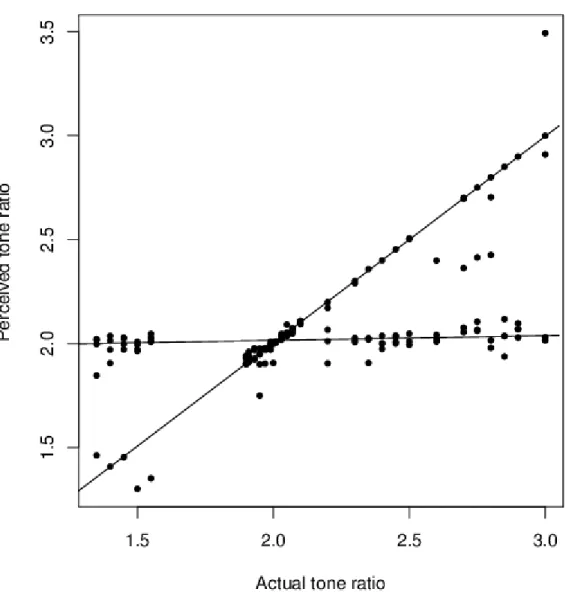
Mixture regression models have been applied in many fields, such as business, marketing, social sciences, and so on. There is a typical data set called tone perception data (Cohen,

1984), which is shown in Figure1.1. In Cohen’s tone perception experiment, a pure funda-mental tone with electronically generated overtones added was played to a trained musician. The overtones were determined by a stretching ratio. The tuning ratio is the ratio between adjusted tone and the fundamental tone. The same musician recorded it for 150 trials. The purposes of this experiment was to see how this tuning ratio affects the perception of the tone and to determine if either of two musical perception theories was reasonable (see Co-hen, 1980 for more detail). Based on Figure 1.1, two lines are evident which correspond to the behavior indicated by the two musical perception theories. The two regression lines cor-respond to correct tuning and tuning to the first overtone, respectively. Such data structure calls for the application of mixture of linear regression.

Let Z be a latent class variable such that given Z =i, the response y depends on the p−dimensional predictor xin a linear way

y =xTβ_i+εi, i= 1,2,· · · , g, (1.12)

where β_i = (βi1,· · · , βip) and εi is independent of x with density fi(·) and mean 0. To

include the intercept in the model, we assume that the first element of x is 1. Suppose P(Z = i) = πi, i = 1,2,· · · , g, and Z is independent of x, then the conditional density of

Y given x, without observingZ, is

f(y|x,θ) = g X i=1 πifi(y;xTβi, σ2i), (1.13) where θ = (π1,β₁, σ₁2, . . . , πg,βg, σg2)T.

1.2.2

Traditional EM algorithm based on normality assumption

The unknown parameterθ in (1.13), given observations {(x1, y1), . . . ,(xn, yn)}, is

tradition-ally estimated by the maximum likelihood estimate (MLE), assuming the error densityfi()

is a normal density with mean 0 and variance σ2

i: ˆ θ = arg max n X log " _g X πiφ(yj;xTjβi, σ 2 i) # , (1.14)

Figure 1.1: The scatter plot of the tone perception data

The predictor is actual tone ratio and the response is the perceived tone ratio by a trained musician.

whereφ(·;µ, σ2_{) is the density function ofN(µ, σ}2_{). Note that the maximizer in (1.14) does} not have an explicit solution and is usually estimated by the EM algorithm:

1. Input initial value: π_i(0), β(0)_i , σ2(0)_i , i= 1, . . . , g.

2. E-step: At (κ+ 1)th _{iteration, we compute conditional expectation of the complete}

data log likelihood, which simplifies to the following calculation:

E(z_ij(κ) |y,θ(κ)) =τ_ij(κ+1) = π (κ) i fi(yj;xTjβi (κ) , σ_i2(κ)) Pg i=1π (κ) i fi(yj;xTjβi (κ) , σ2(_i κ)). (1.15)

3. M-step: update the parameter estimates, ˆθ,

π_i(κ+1) = n X j=1 τ_ij(κ+1)/n, (1.16) β(_iκ+1) = arg min βi n X j=1 τ_ij(κ+1)(yj −xTjβi)(yj −xTjβi) T (1.17) = n X j=1 τ_ij(κ+1)xjxjT !−1 _n X j=1 τ_ij(κ+1)xjyj, σ2(_i κ+1) = Pn j=1τ (κ+1) ij (yj −xTjβ (κ+1) i ) 2 Pn j=1τ (κ+1) ij .

Chapter 2

Robust Mixture Regression Models

The traditional MLE for mixture regression models works well when the error distribution is normal. However, the normality based MLE is sensitive to outliers or heavy-tailed error distributions. Markatou (2000) and Shen et al. (2004) proposed using a weight factor for each data to robustify the estimation procedure for mixture regression models. Neykov et al. (2007) proposed robust fitting of mixtures using the trimmed likelihood estimator (TLE). Bai et al.(2012) proposed a modified EM algorithm to robustly estimate the mixture regression parameters. In this report, we will propose a new robust mixture regression model by extending the mixture of t-distributions proposed by Peel and McLachlan (2000) to the regression setting. We will first review the mixture of t-distributions proposed by McLachlan and Peel (2000).

2.1

Mixture of t-distributions

We denotey1,· · · , ynas p-dimensional random sample with size of n, whereyj isjthrandom

variable, j = 1,2,· · · , n. With location parameter µ, positive-definitep×p scale matrix Σ, degree of freedom ν, we can write the probability density function (p.d.f) of t distribution as f(y;µ,Σ, ν) = Γ( ν+p 2 )|Σ| −1/2 (πν)12pΓ(ν 2){1 +δ(y, µ; Σ)/ν} 1 2(ν+p) ,

where

δ(y;µ; Σ) = (y−µ)TΣ−1(y−µ).

Then, the mixture of t distribution with g-components has the density

f(y;θ) = g X i=1 πif(y;µi,Σi, νi), where θ = π1,· · · , πg−1, ξT,νT T

, ξ = (ξ₁T,· · · , ξ_gT) consists of the elements of the compo-nent means,µ1,· · · , µg, and the distinct elements of the component covariance, Σ1,· · · ,Σg,

ν = (ν1,· · · , νg)T, and πi are nonnegative quantities that sum to one.

Let us consider the maximum-likelihood estimation (MLE) of this g-components mixture t distribution. The MLE of θ is calculate by maximizing the log likelihood function

logL(θ;y) = n X j=1 logf(yj;θ) = n X j=1 log g X i=1 πif(yj;µi,Σi, νi). (2.1)

It is well known that the t-distribution can be considered as a scale mixture of normal distributions. In order to simplify the MLE calculation process, we introduce another latent variable, u. Let u be the latent variable such that

y|u∼N(µ,Σ/u), u∼gamma(1

2ν, 1 2ν),

where N(µ,Σ/u) has density with parameterµand variance Σ/u:

φ(y;µ,Σ/u) = 1

(2π)p/2_|Σ/u|1/2 exp(− 1

2(y−µ)

T_(Σ/u)−1_(y−µ)), and gamma(1₂ν,1₂ν) has density with shape 1₂ν and scale 1₂ν:

f(u;1 2ν, 1 2ν) = 1 Γ(1₂ν)( 1 2ν) −(1₂ν) y(12ν−1)e −2u ν .

Letu= (u1, . . . , un). Then the complete log likelihood function of mixture t distribution

model for (y,z,u) can be written as

logLc(θ;y,z,u) = n X j=1 g X i=1 zijlog{πjφ(yj;µi, σi/uj)f(uj; 1 2νi, 1 2νi)} = n X j=1 g X i=1 zijlogπi+ n X j=1 g X i=1 zijlogφ(yj;µi, σi/uj) + n X j=1 g X i=1 zijlogf(uj; 1 2νi, 1 2νi), (2.2) where, n X j=1 g X i=1 zijlogφ(yj;µi,Σi/uj) = n X j=1 g X i=1 zij −1 2plog(2π)− 1 2|Σi/uj| − 1 2uj(yj −µi) T_(Σ i/uj)−1(yj −µi) , and n X j=1 g X i=1 zijlogf(uj; 1 2νi, 1 2νi) = n X j=1 g X i=1 zij −log Γ(1 2νi)− 1 2νilog( 1 2νi) + 1 2νi(loguj −uj)−loguj . (2.3)

At the (κ+ 1)th iteration, in E-step, we calculate the conditional expectation of the log likelihood function of complete data, E(logLc(θ;y,z,u) | y,θ(κ)). Based on the three

separated parts in the complete log likelihood function logLc(θ;y,z,u), E-step can be done

by calculations of E(zij |y,θ(κ)), E(Uj |y, zij = 1,θ(κ)), and E(logUj |y, zij = 1,θ(κ)).

Hence, the EM algorithm can be written as:

1. Input initial valueθ(0), including π(0)_i , µ(0)_i , Σ(0)_i and ν_i(0).

2. E-step: At the (κ+ 1)th iteration, compute conditional expectation of the complete log likelihood, which contains three parts.

(a) E(zij |y,θ(κ)) = τ (κ+1) ij = π_i(κ)f(yj;µ(iκ),Σ (κ) i , ν (κ) i ) f(yj;θ(κ)) , (2.4)

where, f(yj;µ (κ) i ,Σ (κ) i , ν (κ) i ) = Γ(ν (κ) i +p 2 ) Σ (κ) i −1/2 (π_i(κ)ν_i(κ))12pΓ(ν (κ) i 2 ) n 1 +δ(yj, µ (κ) i ; Σ (κ) i )/ν (κ) i o1₂(νi(κ)+p) , f(yj;θ(κ)) = g X i=1 π(_iκ)f(yj;µ (κ) i ,Σ (κ) i , ν (κ) i ) and δ(yj, µ (κ) i ; Σ (κ) i ) = (yj−µ (κ) i ) T_Σ−(κ) i (yj −µ (κ) i ). (b) E(Uj |y, zij = 1,θ(κ)) = u(ijκ+1) = ν_i(κ)+p ν_i(κ)+δ(yj;µ (κ) i ,Σ (κ) i ) . (2.5) (c) E(logUj |y, zij = 1,θ(κ)) = logu (κ+1) ij + ( ψ(ν (κ) i +p 2 )−log( ν_i(κ)+p 2 ) ) , (2.6) where,ψ(ν (κ) i +p 2 ) = ∂Γ(ν (κ) i +p 2 ) ∂(ν (κ) i +p 2 ) /Γ(ν (κ) i +p 2 ).

3. M-step: At the (κ+ 1)th _{iteration, compute the estimator of parameters (π}

i, µi,Σi, νi)

which maximize the expected complete log likelihood.

π_i(κ+1) = n X j=1 τ_ij(κ+1)/n, (2.7) µ(_iκ+1) = Pn j=1τ (κ+1) ij u (κ+1) ij yj Pn j=1τ (κ+1) ij u (κ+1) ij , (2.8) Σ(_iκ+1) = Pn j=1τ (κ+1) ij u (κ+1) ij (yj −µ (κ+1) i )(yj−µ (κ+1) i )T Pn j=1τ (κ+1) ij . (2.9)

If Σ1 = Σ2 =. . .= Σ, then Σ can be updated by

Σ(κ+1) = Pg i=1 Pn j=1τ (κ+1) ij u (κ+1) ij (yj−µ (κ+1) i )(yj −µ (κ+1) i )T n .

In addition, ν_i(κ+1) is the solution of the following function −ψ(1 2νi)+log( 1 2νi)+1+ 1 n(_iκ+1) n X j=1 τ_ij(κ+1)(logu_ij(κ+1)−u(_ijκ+1))+ψ(ν (κ) i +p 2 )−log( ν_i(κ)+p 2 ) = 0, (2.10) where n(_iκ+1)=Pn j=1τ (κ+1) ij , i= 1,· · · , g.

4. Repeat E-step and M-step until the result can pass certain criterion.

2.2

The proposed robust mixture regression models

by t-distribution

2.2.1

Introduction

In order to robustly estimate the mixture regression parameters in (1.13), we assume that the error density fi(ε) is a t-distribution with degree of freedom νi and scale parameter σi.

Hence, given xj, density function of yj is:

f(yj;xj,θ) = g X i=1 πif(yj;xTjβi, σ 2 i, νi), (2.11) where f(yj;xTjβi, σ 2 i, νi) = Γ(νi+1 2 )|σi| −1 (πiνi) 1 2_Γ(νi 2) 1 +δ(yj,xTjβi;σi2)/νi 1 2(νi+1) , and δ(yj,xTjβi;σi2) = (yj −xTjβi)2/σi2.

Let’s first assume that νis are known. We will talk about how to estimate νis based

on the idea of profile likelihood later. The unknown parameter θ can be estimated by maximizing the log likelihood

n X j=1 log ( _g X i=1 πif(yj;xTjβi, σi2, νi) ) . (2.12)

Note that the complete log likelihood function for (X,y,z) is

logLc(θ;X,y,z) = n X j=1 g X i=1 zijlog{πif(yj;xTjβi, σ 2 i, νi)}, (2.13)

where X = (x1, . . . ,xn)T,y = (y1, . . . , yn),z = (z11,· · · , zng). Based on the theory of EM

algorithm, in E-step, given the current estimate θ(κ) at κth _{iterative M-step, we calculate}

conditional expectation of the complete log likelihoodE(logLc(θ;X,y,z)|X,y,θ(κ)), which

simplifies to the calculation of E(zij | X,y,θ(κ)). In addition, at M-step, we compute the

parameters which maximize

E(logLc(θ;X,y,z)|X,y,θ(κ)) = n X j=1 g X i=1 E(zij |X,y,θ(κ)) log{πif(yj;xTjβi, σ 2 i, νi)}. (2.14) We note that there is no explicit solution for β_i and σ2

i.

Because the t-distribution can be considered as a scale mixture of normal distributions, we use the similar method to simplify M-step in EM algorithm introduced in section 2.1. Let ube the latent variable such that

ε|u∼N(0, σ2/u), u∼gamma(1 2ν,

1

2ν), (2.15)

where gamma(α, γ) has density

f(u;α, γ) = 1 Γ(α)γ

α_uα−1_e−γu_{, u >0.}

Then, marginally ε has a t−distribution with degree of freedom ν and scale parameter σ. Therefore, introducing another latent variable u can simplify the computation of M-step of the proposed EM algorithm.

Note that the complete likelihood for (X,y,u,z) is

logLc(θ;X,y,z,u) (2.16) = n X j=1 g X i=1 zijlog{πiφ(yj;xTjβi, σ 2 i/uj)f(uj; 1 2νi, 1 2νi)} = n X j=1 g X i=1 zijlog(πi) + n X j=1 g X i=1 zijlog{f(uj; 1 2νi, 1 2νi)}, + n X g X zij −1 2log(2πσ 2 i) + 1 2log(uj)− uj 2σ2 i (yj −xTi βi) 2

where u= (u1,· · ·, un) is independent of z.

In addition, the above second term doesn’t involve unknown parameters. Therefore, based on the theory of EM algorithm, in E-step, given the current estimate θ(κ) at κth

step, the calculation of E(logLc(θ;X,y,u,z) | X,y,θ(κ)) simplifies to the calculation of

E(zij |X,y,θ(κ)) and E(uj |X,y,θ(κ), zij = 1). Then in M-step, we find the maximizer of

E(logLc(θ;X,y,u,z)|X,y,θ(κ)) ∝ n X i=1 m X j=1 E(zij |x,θ(κ)) " log(πi)− 1 2log(2πσ 2 i)− E(uj |x,θ(κ), zij = 1) 2σ2 i (yj−xTjβi) 2 # , (2.17) which has explicit solution for θ. Based on the above arguments, we propose the following EM algorithm to maximize (2.12).

1. Input initial value: π_i(0), β(0)_i , and σ2(0)_i .

2. E-step: at the (κ+ 1)th iteration

E(zij |X,y,θ(κ)) = τ (κ+1) ij = π_i(κ)f(yj;xTjβi (κ) , σ_i2(κ), ν_i(κ)) Pg i=1π (κ) i f(yj;xTjβi (κ) , σ2(_i κ), ν_i(κ)) , (2.18) E(uj |X,y,θ(κ), Zij = 1) =u (κ+1) ij = ν_i(κ)+ 1 ν_i(κ)+δ(yj,xTjβi (κ) ;σ2(_i κ), ν_i(κ)), (2.19)

3. M-step: At the (κ+1)th_{iteration, we compute the estimator of parameters (π}

i,βi, σ2i, νi)

which maximize the expected complete log likelihood

π_i(κ+1) = n X j=1 τ_ij(κ+1)/n, (2.20) β(_iκ+1) = n X j=1 xjxjTw (κ+1) ij !−1 _n X j=1 xjyjw (κ+1) ij (2.21) σ_i2(κ+1) = Pn j=1τ (κ+1) ij u (κ+1) ij (yj−xTjβi (κ+1) )2 Pn j=1τ (κ+1) ij (2.22)

where w_ij(κ+1) = τ_ij(κ+1)u_ij(κ+1). If we further assume σ1 =σ2 = · · · = σm = σ, then in

M-step, we can update σ by

σ2 = Pg i=1 Pn j=1τ (κ+1) ij u (κ+1) ij (yj−xTjβi (κ+1) )2 n . (2.23)

4. Repeat E-step and M-step until the result can pass certain criterion.

Based on (2.21) in M-step, we can see that the regression parameters can be considered as a weighted least squares estimate and the weights depend on u(_ijκ+1). From (2.19) in E-step, the weights u(_ijκ+1) decrease if the standardized residuals increase and thus decrease the effects of the outliers to generate the robust estimate for mixture regression parameters. In addition, from (2.22) in M-step, we can see that larger residuals also have smaller effects on σ(_jκ+1) due to the weights u(_ijκ+1).

2.2.2

Trimmed version

The method we introduced in this report, mixture of regression based on t-distribution, is robust when the outliers are in y-direction. However, similar to the traditional M-estimate for linear regression, our method is not robust when the outliers are high leverage points. To solve this problem, we will supply a trimmed version of the new method by fitting the new model to the data after trimming the high leverage points.

We denote X = (x1, . . . ,xn)T and H = X(XTX)−1XT. Let hjj be the jth diagonal of

H, which is so called the leverage for jth predictor xj. Note that

Pn

i=1hjj = p. Based

on Kutner’s theory (2005), a good rule of thumb identifies xj as a high leverage point if

hjj >2p/n. Notice that,

hjj =n−1 + (n−1)−1MDj, (2.24)

where M Dj = (xj−x)¯ TS−1(xj−x) is Mahalanobis distance, ¯¯ xis the sample mean of xjs ,

and S is the sample covariance ofxjs (without the intercept 1). It is well known that ¯x and

high-leverage points. In order to combat this, it is natural to use a modified Mahalanobis distance

M Dj = (xj−m(X))TC(X)−1(xj −m(X))

where m(X) and C(X) are robust estimates of location and scatter for X (after removing the first column 1s).

In this report, we propose to use the minimum covariance determinant (MCD) estimators for m(X) and C(X) and implement it by Fast MCD algorithm of Rousseeuw and Van Driessen (1999). Note that the resulting robust estimate MDj is same as the robust distance

proposed by Rousseeuw and Leroy (1987). After we get the robust estimate MDj, we propose

to trim the data based on the cut pointχ2

p−1,0.975, that is proposed by Pison et al.(2002) to improve the finite-sample efficiency for raw MCD estimator by one-step weighted estimate. Therefore, to make the proposed method also robust against the high leverage outliers, we propose to implement the proposed mixture of regression based on t-distribution after trimming the observations with MDj > χ2p−1,0.975.

One might also employ some other robust estimates for m(X) and C(X). There have been many robust estimators proposed for multivariate location and scatter, such as Stahel-Donoho estimator (Stahel, 1981; Stahel-Donoho, 1982), minimum volume ellipsoid (MVE) estima-tor (Rousseeuw, 1984), S-estimaestima-tor (Rousseeuw and Leroy, 1987; Davies, 1987), and depth based estimator (Donoho and Gasko, 1992; Liu et al., 1999; Zuo and Serfling, 2000; Zuo et al., 2004).

2.2.3

Adaptive choice of the degree of freedom for T-Distribution

by profile likelihood

In previous sections, we assume that the degree of freedom ν for t−distribution is known. In this section, we introduce a method to adaptively choose ν. For simplicity of compu-tation and explanation, we assume that ν1 = ν2 = · · · = νg = ν. However, the method

introduced in this section also applies to the case whenνis are different but with much more

When ν is unknown, it is natural to estimate ν and mixture regression parameter θ by maximizing the log-likelihood (2.12) over both ν and θ. However, based on Peel and McLachlan (2000), there is no explicit solution for ν in the M-step. In order to overcome this difficult, we define the profile likelihood for ν:

L(ν) = max θ n X j=1 log ( _g X i=1 πif(yj;xTjβi, σ 2 i, ν) ) (2.25)

For each fixed ν, we can easily findL(ν) based on the proposed EM algorithm in section 2.2.1. Then we can estimate ν by

ˆ

ν = arg max

ν L(ν).

In practice, we can calculate L(ν) in a set of grid points of ν, say ν = 1, . . . , νmax. We should notice that when ν is large enough, the t-distribution is close to normal distribution. Actually, νmax need not be too large; usually 15 to 20 is large enough for the purpose.

Chapter 3

Simulation Study and Application

In this section, we use the simulation study to demonstrate the effectiveness of the proposed method and compare it with some of the existing estimation methods. To compare different methods, we report the mean squared errors (MSE) and bias of the parameter estimates for each estimation method. Note, however, for mixture models, there are well known label switching issues (Celeux, Hurn, and Robert, 2000; Stephens, 2000; Yao and Lindsay, 2009; Yao, 2012a, 2012b) when doing comparison using the simulation study. There are no widely accepted labeling methods. In our simulation study, we simply choose the labels by minimizing the distance to the true parameter values. However, it requires more research to compare different labeling methods.

Note that the log-likelihood function (2.12) is unbounded and goes to infinity if one observation exactly lies on one component line and the corresponding component variance goes to zero. There has been great research efforts in dealing with the unbounded likelihood issue. See, for example, Hathaway (1985, 1986), Chen, Tan, and Zhang (2008), and Yao (2010). In our simulation study, for simplicity of computation, we assume equal variance for each component.

We generate the independent and identically distributed (i.i.d.) data {(x1j, x2j, yj), j =

1, . . . , n} from the model Y =

0 +X1+X2+1, if Z = 1; 0−X1−X2 +2, if Z = 2.

where Z is a component indicator of Y with P(Z = 1) = 0.25, X1 ∼N(0,1), X2 ∼N(0,1), and 1 and 2 have the same distribution as . We estimate the above mixture regression parameters by the following five methods:

1. traditional MLE based on normality assumption (MLE)

2. trimmed likelihood estimator (TLE) proposed by Neykov et al. (2007) with the per-centage of trimmed data α set to 0.1 (The choice of α plays an important role for the TLE. If α is too large, the TLE will lose much efficiency. If α is too small and the percentage of outliers is more than α, then the TLE will fail. In our simulation study, the proportion of outliers is never greater than 0.1.)

3. the robust modified EM algorithm based on bisquare (MEM-bisquare) proposed by Bai et al. (2012).

4. the proposed robust mixture regression based on t-distribution (Mixregt)

5. the proposed trimmed version of Mixregt (Mixregt-trim)

In order to compare the performance of different methods, we consider the following five cases for the error density of :

Case I: ∼N(0,1) – standard normal distribution. Case II: ∼t3 – t-distribution with degrees of freedom 3.

Case III: ∼t1 – t-distribution with degrees of freedom 1 (Cauchy distribution). Case IV: ∼0.95N(0,1) + 0.05N(0,52_{) – contaminated normal mixture.}

Case V: ∼ N(0,1) with 5% of high leverage outliers being X1 = 20, X2 = 20, and Y = 100.

Case I is used to test the efficiency of different estimation methods compared to the traditional MLE when the error is exactly normally distributed and there are no outliers. Case II is a heavy-tailed distribution. Thet-distributions with degrees of freedom from 3 to 5 are often used to represent the heavy-tailed distributions. Case III is a Cauchy distribution which has an extremely heavy-tailed. The contaminated normal mixture model in Case IV is often used to mimic the outlier situation. The 5% data from N(0,52_{) are likely to be low} leverage outliers. In Case V, 95% of the observations have the error distribution N(0,1), but 5% of the observations are replicated high leverage outliers with X1 = 20, X2 = 20, and Y = 100.

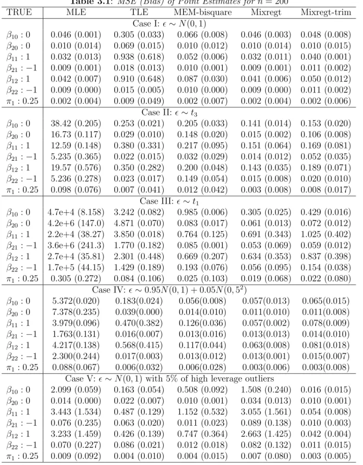
Tables 3.1 and 3.2 report the mean squared errors (MSE) and absolute bias (Bias) of the parameter estimates for each estimation method for sample size n = 200 and n = 400, respectively. The number of replicates is 200. Based on Tables 3.1 and 3.2, we can see that Mixregt and Mixregt-trim have overall better or comparable performance than other three methods considered for Case I to IV. For Case V, when there are high leverage outliers, Mixregt-trim still works well and works much better than the other four methods, specifically, we have the following findings:

1. The MLE works the best for Case I ( ∼ N(0,1)), but fails to provide reasonable estimates for Case II to V.

2. Mixregt and Mixregt-trim have better performance than MEM-bisquare for Case I, II, and IV when n = 200, but have close performance to MEM-bisquare when n= 400.

3. Mixregt, Mixregt-trim, and MEM-bisquare have overall better performance than TLE for Case I to IV.

4. For Case V, when there are high leverage outliers, Mixregt-trim works the best. In addition, TLE and MEM-bisquare also work better than Mixregt and MLE.

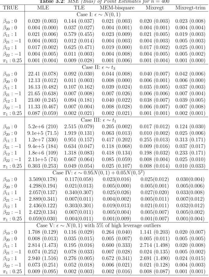
In order to check the performance of the proposed profile likelihood for the selection of degree of freedom for t−distribution, in Table 3.3, we report the mean and median of

estimated degrees of freedom for Mixregt and Mixregt-trim. The degrees of freedom are chosen based on the grid points from [1, vmax], where vmax = 15 is chosen in our simulation study. Therefore, for Case I−normal distribution, the “optimal” solution is vmax = 15. Based on the results of Case I, II, and III in Table 3.3, the proposed profile likelihood can adaptively estimate the degree of freedom for t−distribution. For Case IV, although the true error density is not a t-distribution, both Mixregt and Mixregt-trim are able to use a heavy-tailed t-distribution to approximate the contaminated normal mixture to produce a robust estimate for mixture regression parameters. For Case V, the estimated degrees of freedom for Mixregt-trim are close to vmax = 15. Therefore, Mixregt-trim successfully trimmed the high leverage outliers and recovered the original normal error density.

Table 3.1: MSE (Bias) of Point Estimates for n = 200

TRUE MLE TLE MEM-bisquare Mixregt Mixregt-trim

Case I: ∼N(0,1) β10 : 0 0.046 (0.001) 0.305 (0.033) 0.066 (0.008) 0.046 (0.003) 0.048 (0.008) β20 : 0 0.010 (0.014) 0.069 (0.015) 0.010 (0.012) 0.010 (0.014) 0.010 (0.015) β11 : 1 0.032 (0.013) 0.938 (0.618) 0.052 (0.006) 0.032 (0.011) 0.040 (0.001) β21 :−1 0.009 (0.001) 0.018 (0.013) 0.010 (0.001) 0.009 (0.001) 0.011 (0.002) β12 : 1 0.042 (0.007) 0.910 (0.648) 0.087 (0.030) 0.041 (0.006) 0.050 (0.012) β22 :−1 0.009 (0.000) 0.015 (0.005) 0.010 (0.000) 0.009 (0.000) 0.011 (0.002) π1 : 0.25 0.002 (0.004) 0.009 (0.049) 0.002 (0.007) 0.002 (0.004) 0.002 (0.006) Case II: ∼t3 β10 : 0 38.42 (0.205) 0.253 (0.021) 0.205 (0.033) 0.141 (0.014) 0.153 (0.020) β20 : 0 16.73 (0.117) 0.029 (0.010) 0.148 (0.020) 0.015 (0.002) 0.106 (0.008) β11 : 1 12.59 (0.148) 0.380 (0.331) 0.217 (0.095) 0.151 (0.064) 0.169 (0.081) β21 :−1 5.235 (0.365) 0.022 (0.015) 0.032 (0.029) 0.014 (0.012) 0.052 (0.035) β12 : 1 19.57 (0.576) 0.350 (0.282) 0.200 (0.048) 0.143 (0.035) 0.189 (0.071) β22 :−1 5.236 (0.278) 0.023 (0.017) 0.149 (0.054) 0.015 (0.008) 0.020 (0.010) π1 : 0.25 0.098 (0.076) 0.007 (0.041) 0.012 (0.042) 0.003 (0.008) 0.008 (0.017) Case III: ∼t1 β10 : 0 4.7e+4 (8.158) 3.242 (0.082) 0.985 (0.006) 0.305 (0.025) 0.429 (0.016) β20 : 0 4.2e+6 (147.0) 4.871 (0.070) 0.083 (0.017) 0.061 (0.013) 0.072 (0.012) β11 : 1 2.2e+4 (38.27) 3.850 (0.018) 0.764 (0.125) 0.691 (0.343) 1.025 (0.402) β21 :−1 3.6e+6 (241.3) 1.770 (0.182) 0.085 (0.001) 0.053 (0.069) 0.059 (0.012) β12 : 1 2.7e+4 (35.81) 2.301 (0.448) 0.669 (0.207) 0.634 (0.353) 0.837 (0.398) β22 :−1 1.7e+5 (44.15) 1.429 (0.189) 0.193 (0.076) 0.056 (0.095) 0.154 (0.038) π1 : 0.25 0.305 (0.272) 0.084 (0.106) 0.025 (0.103) 0.019 (0.068) 0.022 (0.080) Case IV: ∼0.95N(0,1) + 0.05N(0,52) β10 : 0 5.372(0.020) 0.183(0.024) 0.056(0.008) 0.057(0.013) 0.065(0.015) β20 : 0 7.378(0.235) 0.039(0.000) 0.014(0.010) 0.011(0.010) 0.011(0.008) β11 : 1 3.979(0.096) 0.470(0.382) 0.126(0.036) 0.057(0.002) 0.078(0.009) β21 :−1 1.763(0.131) 0.016(0.007) 0.013(0.016) 0.013(0.013) 0.014(0.010) β12 : 1 4.217(0.138) 0.568(0.415) 0.117(0.044) 0.063(0.008) 0.081(0.018) β22 :−1 2.300(0.244) 0.017(0.003) 0.013(0.012) 0.013(0.001) 0.015(0.007) π1 : 0.25 0.088(0.067) 0.006(0.032) 0.006(0.028) 0.003(0.006) 0.003(0.008)

Case V: ∼N(0,1) with 5% of high leverage outliers

β10 : 0 2.099 (0.059) 0.163 (0.054) 0.508 (0.092) 1.508 (0.240) 0.016 (0.015) β20 : 0 0.014 (0.000) 0.022 (0.007) 0.010 (0.001) 0.034 (0.013) 0.010 (0.001) β11 : 1 3.443 (1.534) 0.487 (0.129) 1.152 (0.532) 3.055 (1.561) 0.054 (0.008) β21 :−1 0.076 (0.235) 0.063 (0.020) 0.011 (0.023) 0.089 (0.138) 0.010 (0.003) β12 : 1 3.233 (1.459) 0.426 (0.139) 0.747 (0.364) 2.663 (1.425) 0.042 (0.004) β22 :−1 0.070 (0.227) 0.086 (0.021) 0.012 (0.018) 0.082 (0.132) 0.011 (0.015) π1 : 0.25 0.009 (0.092) 0.004 (0.010) 0.004 (0.015) 0.007 (0.080) 0.003 (0.005)

Table 3.2: MSE (Bias) of Point Estimates for n = 400

TRUE MLE TLE MEM-bisquare Mixregt Mixregt-trim

Case I: ∼N(0,1) β10: 0 0.020 (0.003) 0.144 (0.037) 0.021 (0.003) 0.020 (0.003) 0.023 (0.008) β20: 0 0.004 (0.000) 0.037 (0.027) 0.004 (0.001) 0.004 (0.001) 0.004 (0.004) β11: 1 0.021 (0.006) 0.579 (0.455) 0.023 (0.009) 0.021 (0.005) 0.019 (0.003) β21:−1 0.004 (0.003) 0.012 (0.014) 0.004 (0.003) 0.004 (0.003) 0.005 (0.003) β12: 1 0.017 (0.002) 0.625 (0.471) 0.019 (0.000) 0.017 (0.002) 0.025 (0.001) β22:−1 0.004 (0.005) 0.011 (0.003) 0.004 (0.008) 0.004 (0.005) 0.005 (0.002) π1 : 0.25 0.001 (0.004) 0.009 (0.028) 0.001 (0.006) 0.001 (0.004) 0.001 (0.000) Case II: ∼t3 β10: 0 22.41 (0.078) 0.092 (0.030) 0.044 (0.008) 0.040 (0.007) 0.042 (0.006) β20: 0 12.13 (0.012) 0.011 (0.003) 0.008 (0.000) 0.006 (0.001) 0.006 (0.000) β11: 1 16.13 (0.482) 0.107 (0.162) 0.039 (0.024) 0.035 (0.005) 0.037 (0.003) β21:−1 21.65 (0.638) 0.007 (0.008) 0.007 (0.026) 0.006 (0.006) 0.007 (0.004) β12: 1 23.00 (0.245) 0.094 (0.181) 0.040 (0.022) 0.038 (0.007) 0.039 (0.005) β22:−1 11.33 (0.467) 0.007 (0.004) 0.008 (0.028) 0.006 (0.007) 0.007 (0.008) π1 : 0.25 0.087 (0.059) 0.002 (0.021) 0.002 (0.021) 0.001 (0.001) 0.002 (0.001) Case III: ∼t1 β10: 0 5.2e+6 (210) 2.515 (0.079) 0.205 (0.002) 0.017 (0.012) 0.124 (0.030) β20: 0 9.1e+5 (71.5) 1.919 (0.131) 0.063 (0.013) 0.010 (0.002) 0.025 (0.006) β11: 1 1.2e+7 (330) 0.951 (0.157) 0.417 (0.202) 0.255 (0.013) 0.313 (0.171) β21:−1 9.4e+5 (184) 0.634 (0.047) 0.118 (0.068) 0.009 (0.016) 0.037 (0.017) β12: 1 1.8e+6 (109) 1.318 (0.083) 0.418 (0.134) 0.198 (0.032) 0.233 (0.171) β22:−1 2.11e+5 (74) 0.667 (0.064) 0.085 (0.059) 0.008 (0.004) 0.025 (0.010) π1 : 0.25 0.303 (0.253) 0.049 (0.054) 0.025 (0.107) 0.008 (0.014) 0.010 (0.033) Case IV: ∼0.95N(0,1) + 0.05N(0,52) β10: 0 3.509(0.178) 0.117(0.058) 0.023(0.016) 0.025(0.012) 0.030(0.004) β20: 0 4.298(0.194) 0.021(0.013) 0.005(0.000) 0.005(0.001) 0.005(0.006) β11: 1 2.057(0.137) 0.340(0.307) 0.025(0.026) 0.027(0.020) 0.033(0.008) β21:−1 2.889(0.341) 0.007(0.011) 0.004(0.002) 0.005(0.011) 0.007(0.012) β12: 1 2.436(0.122) 0.303(0.301) 0.019(0.013) 0.021(0.011) 0.032(0.012) β22:−1 2.422(0.134) 0.007(0.011) 0.005(0.004) 0.005(0.007) 0.005(0.002) π1 : 0.25 0.059(0.030) 0.004(0.011) 0.001(0.009) 0.001(0.007) 0.001(0.004)

Case V: ∼N(0,1) with 5% of high leverage outliers

β10: 0 1.708 (0.129) 0.116 (0.029) 0.264 (0.040) 1.141 (0.203) 0.020 (0.007) β20: 0 0.008 (0.013) 0.035 (0.015) 0.005 (0.007) 0.005 (0.011) 0.005 (0.005) β11: 1 2.814 (1.473) 0.195 (0.016) 0.600 (0.333) 2.714 (1.498) 0.020 (0.008) β21:−1 0.074 (0.252) 0.078 (0.033) 0.007 (0.028) 0.024 (0.135) 0.005 (0.002) β12: 1 2.940 (1.516) 0.276 (0.005) 0.672 (0.341) 2.691 (1.490) 0.024 (0.015) β22:−1 0.073 (0.251) 0.052 (0.018) 0.006 (0.021) 0.021 (0.128) 0.004 (0.003) π : 0.25 0.009 (0.095) 0.002 (0.003) 0.002 (0.016) 0.008 (0.087) 0.001 (0.001)

Table 3.3: The mean (median) of estimated degree freedom by Mixregt and Mixregt-trim based on the grid points from [1,15].

Case n Mixregt Mixregt-trim

I: ∼N(0,1) 200 14.5 (15) 14.4 (15) 400 14.7 (15) 14.8 (15) II: ∼t3 200 3.33 (3) 3.39 (3) 400 3.18 (3) 3.18 (3) III: ∼t1 200 1 (1) 1 (1) 400 1 (1) 1 (1) IV: ∼0.95N(0,1) + 0.05N(0,52_{) 200 3.52(3) 3.45 (3)} 400 3.91(3) 3.92 (3) V: ∼N(0,1) with 5% high leverage outliers 200 4.62 (4) 13.8 (15)

Chapter 4

Discussion

In this report, we proposed a new robust mixture of regression based on t-distribution and profile likelihood. However, such proposed model is not robust to outliers with high leverage outliers. We further proposed a trimmed version of the proposed method by fitting the new model after adaptively trimming the high leverage points. The simulation study demonstrated the effectiveness of the proposed new method.

For the trimmed version of the new method, we used the same weights as Pison et al. (2002), i.e, delete the high leverage points based on the cut point χ2

p−1,0.975. However, some high leverage points might have small residuals and thus can also provide valuable information to the regression parameters. It requires more research how to incorporate information from the data with high leverage points but with small residuals. One possible way is to borrow the ideas from GM-estimators (Krasker and Welsch, 1982; Maronna and Yohai, 1981) and one-step GM-estimators (Coakley and Hettmansperger, 1993; Simpson and Yohai, 1998).

In addition, it is also interesting to provide the sample breakdown points for the pro-posed method and some of other robust mixture regression models. However, we should note that the analysis of breakdown point for traditional linear regression can’t be directly applied to mixture regression. For example, the breakdown point of TLE for traditional linear regression doesn’t apply to the mixture regression, due to its special cluster proper-ties. Garc´ıa-Escudero et al. (2010) also stated that the traditional definition of breakdown

point is not the right one to quantify the robustness of clustering regression procedures to outliers, since the robustness of these procedures is not only data dependent but also cluster dependent, since the outliers might create a new cluster.

Bibliography

[1] Bai, X., Yao, W., and Boyer, J. E. (2012). Robust fitting of mixture regression models. Computational Statistics and Data Analysis, 56, 2347-2359.

[2] Celeux, G., Hurn, M., and Robert, C. P. (2000). Computational and inferential diffi-culties with mixture posterior distributions. Journal of the American Statistical Asso-ciation, 95, 957-970.

[3] Chen, J., Tan, X., and Zhang, R. (2008). Inference for normal mixture in mean and variance. Statistica Sincia, 18, 443-465.

[4] Coakley, C. W. and Hettmansperger, T. P. (1993). A bounded influence, high break-down, efficient regression estimator. Journal of the American Statistical Association, 88, 872-880.

[5] Cohen, E. (1980). Inharmonic Tone Perception, PhD thesis, Stanford University, un-published.

[6] Cohen, E. (1984). Some effects of inharmonic partials on interval perception. Music Perception, 1, 323-349.

[7] Day, N.E. (1969). Estimating the components of a mixture of two normal distributions. Biometrika 56, 463-474.

[8] Davies, L. (1987). Asymptotic behavior of S-estimators of multivariate location param-eters and dispersion matrices. Annals of Statistics, 15, 1269-1292.

[9] Dempster, A. P., Laird, N. M., and Rubin, D. B. (1977). Maximum likelihood from incomplete data via the EM algorithm (with discussion). Journal of Royal Statistical

[10] Donoho, D. L. (1982). Breakdown properties of multivariate location estimators. Qual-ifying paper, Harvard University, Boston.

[11] Donoho, D. L. and Gasko, M. (1992). Breakdown properties of location estimates based on halfspace depth and projected outlyingness. Annals of Statistics, 20, 1803-1827.

[12] Garc´ıa-Escudero, L. A., Gordaliza, A., Mayo-Iscara, A., and San Mart´ın, R. (2010). Ro-bust clusterwise linear regression through trimming. Computational Statistics & Data Analysis, 54, 3057-3069.

[13] Hathaway, R. J. (1985). A constrained formulation of maximum-likelihood estimation for normal mixture distributions. Annals of Statistics, 13, 795-800.

[14] Hathaway, R. J. (1986). A constrained EM algorithm for univariate mixtures. Journal of Statistical Computation and Simulation, 23, 211-230.

[15] Krasker, W. S. and Welsch, R. E. (1982). Efficient bounded influence regression esti-mation. Journal of the American Statistical Association, 77, 595-604.

[16] Kutner, M.H., C.J. Nachtsheim, J. Neter and W. Li. (2005). Applied Linear Statistical Models. 5th Edn.New York: McGraw-Hill.

[17] Liu, R. Y., Parelius, J. M. and Singh, K. (1999). Multivariate analysis by data depth: Descriptive statistics, graphics and inference. Annals of Statistics, 27, 783-840.

[18] Markatou, M. (2000). Mixture models, robustness, and the weighted likelihood method-ology. Biometrics, 56, 483-486.

[19] Maronna, R. A. and Yohai, V. J. (1981). Asymptotic behavior of general M-estimators for regression and scale with random carriers. Probability Theory and Related Fields, 58, 7-20.

[21] Newcomb, S. (1886). A generalized theory of the combination of obsevations so as to obtain the best result. American Journal of Mathematics8, 343-366.

[22] Neykov, N., Filzmoser, P., Dimova, R., and Neytchev, P. (2007). Robust fitting of mixtures using the trimmed likelihood estimator. Computational Statistics and Data Analysis, 52, 299-308.

[23] Pearson, K. (1894). Contributions to the theory of mathematical evolution.Philosophical Transactions of the Royal Society of LondonA 185,71-110.

[24] Peel, D. and McLachlan, G. J. (2000). Robust mixture modelling using the t distribution Statistics and Computing, 10, 339-348.

[25] Pison, G., Van Aelst, S. and Willems, G. (2002). Small sample corrections for LTS and MCD. Metrika, 55, 111-123.

[26] Rosseeuw, P. J. (1984). Least median of squares regression. Journal of the American Statistical Association, 79, 871-880.

[27] Rousseeuw, P. J. and Leroy, A. M. (1987). Robust Regression and Outlier Detection. Wiley-Interscience, New York.

[28] Rosseeuw, P. J. and van Zomeren, B. C. (1990). Unmasking multivariate outliers and leverate points. Journal of the American Statistical Association, 85, 633-639.

[29] Rousseeuw, P. J. and Van Driessen, K. (1999). A fast algorithm for the minimum covariance determinant estimator. Technometrics, 41, 212-223.

[30] Shen, H., Yang, J., and Wang, S. (2004). Outlier detecting in fuzzy switching regression models. Artificial Intelligence: Methodology, Systems, and Applications Lecture Notes in Computer Science, 2004, Vol. 3192/2004, 208-215.

[32] Stahel, W. A. (1981). Robuste Sch¨atzungen: Infinitesimale Optimalit¨at und Sch¨atzungen von Kovarianzmatrizen. Ph.D. thesis, ETH Z¨urich.

[33] Stephens, M. (2000). Dealing with label switching in mixture models. Journal of Royal Statistical Society, Ser B., 62, 795-809.

[34] Wolfe, J.H. (1965). A computer program for the computation of maximum likelihood analysis of types.Research Memo. SRM65-12. SanDiego: U.S. Naval Personnel Research Activity.

[35] Wolfe, J.H. (1967). NORMIX: Computation methods fro estimating the parameters of multivariate normal mixtures of distribution. Research Memo. SRM68-2. SanDiego: U.S. Naval Personnel Research Activity.

[36] Yao, W. and Lindsay, B. G. (2009). Bayesian mixture labeling by highest posterior density. Journal of American Statistical Association, 104, 758-767.

[37] Yao, W. (2010). A profile likelihood method for normal mixture with unequal variance. Journal of Statistical Planning and Inference, 140, 2089-2098.

[38] Yao, W. (2012a). Bayesian mixture labeling and clustering.Communications in Statis-tics - Theory and Methods, 41, 403-421.

[39] Yao, W. (2012b). Model based labeling for mixture models. Statistics and Computing. 22, 337-347.

[40] Zuo, Y., Cui, H. and He, X. (2004). On the Stahel-Donoho estimator and depth-weighted means of multivariate data. Annals of Statistics, 32, 167-188.

[41] Zuo, Y. and Serfling, R. (2000). General notions of statistical depth function. Annals of Statistics, 28, 461-482.

Appendix A

R-Programs

rm (list = ls ()) library(MASS); library(gregmisc) library(robustbase) huberpsi<-function(t,k=1.345){ out=pmax(-k,pmin(k,t));out} bisquare<-function(t,k=4.685){out=t*pmax(0,(1-(t/k)^2))^2;out} biscalew<-function(t){ t[which(t==0)]=min(t[which(t!=0)])/10; out=pmin(1-(1-t^2/1.56^2)^3,1)/t^2;out}

##the EM algorithm to fit the mixture of linear regression

#mixlinone estimates the mixture regression parameters by MLE based on ONE initial value

mixlinone<-function(x,y,bet,sig,pr,m=2){ run=0; n=length(y);

X=cbind(rep(1,n),x);

r=matrix(rep(0,m*n),nrow=n);pk=r;lh=0; for(j in seq(m)) {r[,j]=y-X%*%bet[j,];lh=lh+pr[j]*dnorm(r[,j],0,sig[j]);} lh=sum(log(lh)); #E-steps repeat { prest=c(bet,sig,pr);run=run+1;plh=lh; for(j in seq(m)) { pk[,j]=pr[j]*pmax(10^(-300),dnorm(r[,j],0,sig[j]))} pk=pk/matrix(rep(apply(pk,1,sum),m),nrow=n); #M-step np=apply(pk,2,sum);pr=np/n;lh=0; for(j in seq(m)) {w=diag(pk[,j]); bet[j,]=ginv(t(X)%*%w%*%X)%*%t(X)%*%w%*%y; r[,j]= y-X%*%bet[j,]; sig[j]=sqrt(t(pk[,j])%*%(r[,j]^2)/np[j]); lh=lh+pr[j]*dnorm(r[,j],0,sig[j]);} lh=sum(log(lh));dif=lh-plh; if(dif<10^(-5)|run>500){break}}}

else{ #the case when the variance is equal r=matrix(rep(0,m*n),nrow=n);pk=r; lh=0

for(j in seq(m))

{r[,j]=y-X%*%bet[j,];lh=lh+pr[j]*dnorm(r[,j],0,sig);} lh=sum(log(lh));

#E-steps repeat { prest=c(bet,sig,pr);run=run+1;plh=lh; for(j in seq(m)) { pk[,j]=pr[j]* pmax(10^(-300),dnorm(r[,j],0,sig)) } pk=pk/matrix(rep(apply(pk,1,sum),m),nrow=n); #M-step np=apply(pk,2,sum);pr=np/n; for(j in seq(m)) { w=diag(pk[,j]); bet[j,]=ginv(t(X)%*%w%*%X)%*%t(X)%*%w%*%y; r[,j]= y-X%*%bet[j,]; } sig=sqrt(sum(pk*(r^2))/n);lh=0; for(j in seq(m)) {lh=lh+pr[j]*dnorm(r[,j],0,sig);} lh=sum(log(lh)); dif=lh-plh; if(dif<10^(-5)|run>500){break}} sig=sig*rep(1,m)} est=list(theta= matrix(c(bet,sig,pr),nrow=m),likelihood=lh,run=run,diflh=dif) est}

##mixlin based on 20 initial values

{ n=length(y); x=matrix(x,nrow=n) a=dim(x);p=a[2]+1; n1=2*p; bet= matrix(rep(0,k*p),nrow=k);sig=0; for(j in seq(k)) {ind=sample(1:n,n1); X=cbind(rep(1,n1),x[ind,]); bet[j,]=ginv(t(X)%*%X)%*%t(X) %*%y[ind]; sig=sig+sum((y[ind] -X%*%bet[j,])^2);} pr=rep(1/k,k);sig=sig/n1/k; est=mixlinone(x,y,bet,sig,pr,k);lh=est$likelihood; obj=rep(0,numini); obj[1]=lh; for(i in seq(numini-1)) {bet= matrix(rep(0,k*p),nrow=k);sig=0; for(j in seq(k)) {ind=sample(1:n,n1); X=cbind(rep(1,n1),x[ind,]); bet[j,]=ginv(t(X)%*%X)%*%t(X) %*%y[ind]; sig=sig+sum((y[ind] -X%*%bet[j,])^2);} pr=rep(1/k,k);sig=sig/n1/k;pest=est;plh=lh; est=mixlinone(x,y,bet,sig,pr,k);lh=est$likelihood;obj[i+1]=lh; if(lh<plh){est=pest;lh=plh;}} est=list(theta=est$theta,likelihood=est$likelihood,run=est$run,diflh=est$dif,objlh=obj) est}

##the robust EM algorithm to fit the mixture of linear regression based on bisquare function

using bisquare function #based on one initial value mixlinrb_bione<-function(x,y,bet,sig,pr,m=2){ run=0;acc=10^(-4)*max(abs(c(bet,sig,pr))); n=length(y); X=cbind(rep(1,n),x);p=dim(X)[2]; if(length(sig)>1) { r=matrix(rep(0,m*n),nrow=n);pk=r; for(j in seq(m)) r[,j]=(y-X%*%bet[j,])/sig[j]; #E-steps repeat { prest=c(sig,bet,pr);run=run+1; for(j in seq(m)) { pk[,j]=pr[j]*pmax(10^(-300),dnorm(r[,j],0,1))/sig[j] } pk=pk/matrix(rep(apply(pk,1,sum),m),nrow=n); #M-step np=apply(pk,2,sum);pr=np/n; r[which(r==0)]=min(r[which(r!=0)])/10; for(j in seq(m)) { w=diag(pk[,j]*bisquare(r[,j])/r[,j]); bet[j,]= solve(t(X)%*%w%*%X+10^(-10)*diag(rep(1,p)))%*%t(X)%*%w%*%y; r[,j]= (y-X%*%bet[j,])/sig[j];

sig[j]=sqrt(sum(r[,j]^2*sig[j]^2*pk[,j]*biscalew(r[,j]))/np[j]/0.5); } dif=max(abs(c(sig,bet,pr)-prest)) if(dif<acc|run>500){break} } } else{ r=matrix(rep(0,m*n),nrow=n);pk=r; for(j in seq(m)) r[,j]=( y-X%*%bet[j,])/sig; #E-steps repeat { prest=c(sig,bet,pr);run=run+1; for(j in seq(m)) { pk[,j]=pr[j]* pmax(10^(-300),dnorm(r[,j],0,1))/sig } pk=pk/matrix(rep(apply(pk,1,sum),m),nrow=n); #M-step np=apply(pk,2,sum);pr=np/n; r[which(r==0)]=min(r[which(r!=0)])/10; for(j in seq(m)) { w=diag(pk[,j]*bisquare(r[,j])/r[,j]); bet[j,]=solve(t(X)%*%w%*%X+10^(-10)*diag(rep(1,p)))%*%t(X)%*%w%*%y; r[,j]=( y-X%*%bet[j,])/sig; } sig=sqrt(sum(pk*(r^2*sig[1]^2)*biscalew(r))/n/0.5)

dif=max(abs(c(sig,bet,pr)-prest)) if(dif<acc|run>500){break} } sig=rep(sig,m); } theta=matrix(c(bet,sig,pr),nrow=m); est=list(theta=theta,difpar=dif,run=run) est }

## mixlinrb_bi estimates the mixture regression parameters robustly using bisquare function #based on multiple initial values.

The solution is found by the modal solution

mixlinrb_bi<-function(x,y,m=2, numini=20) { n=length(y); x=matrix(x,nrow=n);a=dim(x);p=a[2]+1; n1=2*p; perm=permutations(m,m);sig=0;ind1=c(); for(j in seq(m)) { ind1= sample(1:n,n1); X=cbind(rep(1,n1),x[ind1,]); bet[j,]=ginv(t(X)%*%X)%*%t(X) %*%y[ind1]; sig=sig+sum((y[ind1] -X%*%bet[j,])^2);} pr=rep(1/m,m);sig=max(sig/n1/m); est=mixlinrb_bione(x,y,bet,sig,pr,m); lenpar=length(c(est$theta)); theta= matrix(rep(0,lenpar*(numini)),ncol=lenpar); theta[1,]=c(est$theta); minsig=10^(-1)*sig; trimbet=matrix(theta[1,1:(p*m)],nrow=m);

trimbet=matrix(rep(matrix(t(trimbet),ncol=p*m,byrow=T),gamma(m+1)), ncol=p*m,byrow=T); ind=matrix(rep(0,numini),nrow=1);ind[1]=1;numsol=1;solindex=1; sol=matrix(theta[1,],nrow=1); for(i in 2:numini) {sig=0;ind1=c(); for(j in seq(m)) { ind1= sample(1:n,n1); X=cbind(rep(1,n1),x[ind1,]); bet[j,]=ginv(t(X)%*%X)%*%t(X) %*%y[ind1]; sig=sig+sum((y[ind1] -X%*%bet[j,])^2);} pr=rep(1/m,m);sig=max(sig/n1/m,minsig); est=mixlinrb_bione(x,y,bet,sig,pr,m); theta[i,]=est$theta; temp= matrix(theta[i,1:(p*m)],nrow=m);temp=matrix(t(temp[t(perm),]), ncol=p*m,byrow=T); dif=apply((trimbet-temp )^2,1,sum);temp1=which(dif==min(dif)); theta[i,]=c(c(matrix(temp[temp1[1],],nrow=m,byrow=T)), theta[i,p*m+perm[temp1[1],]],theta[i,p*m+m+perm[temp1[1],]]); dif=apply((matrix(rep(theta[i,1:(p*m)],numsol), nrow=numsol,byrow=T)-sol[,1:(p*m)])^2,1,sum); if(min(dif)>0.1){sol=rbind(sol,theta[i,]); numsol=numsol+1; solindex=c(solindex,i); ind=rbind(ind,rep(0,numini)); ind[numsol,i]=1}else{ind1=which(dif==min(dif));ind[ind1,i]=1;} } num=apply(ind,1,sum); ind1=order(-num); bestindex=ind1;

for(j in seq(numsol)) {if(min(sol[ind1[j], (p*m+m+1):(p*m+2*m)])>0.05) {index=1; est=matrix(sol[ind1[j],],nrow=m); for(l in seq(m-1)) {temp=matrix(rep(est[l,1:p],m-l),nrow=m-l, byrow=T)-est[(l+1):m,1:p]; temp=matrix(temp,nrow=m-l); dif=apply(temp^2,1,sum);if(min(dif)<0.1){index=0;break} } if(index==1){bestindex=ind1[j];break}}} est= sol[bestindex[1],]; out=list(theta=est,estall=theta, uniqueest=sol, countuniqueest=num,uniqueestindex=solindex, bestindex=solindex[bestindex],estindex=ind);out }

##trimmed likelihood estimator

#trimmixone uses the trimmed likelihood estimator based on ONE initial value. trimmixone<-function(x,y,k=2,alpha=0.9,bet,sig,pr){

n=length(y);n1=round(n*alpha); x=matrix(x,nrow=n);a=dim(x);p=a[2]+1; X=cbind(rep(1,n),x); if(dim(bet)[2]==k) bet=t(bet);

lh=0 for (i in seq(k)) { lh=lh+pr[i]*dnorm(y-X%*%bet[i,],0,sig[1])} ind=order(-lh);run=0; acc=10^(-4); obj=sum(log(lh[ind[1:n1]])); repeat

{pobj=obj;run=run+1; x1=x[ind[1:n1],];y1=y[ind[1:n1]]; fit=mixlinone(x1,y1,bet,sig,pr,k);fit=fit$theta; bet=matrix(fit[1:(p*k)],nrow=k);sig=fit[p*k+1]; pr=fit[(p*k+k+1):(p*k+2*k)];lh=0; for(i in seq(k)) {lh=lh+pr[i]*dnorm(y-X%*%bet[i,],0,sig[1]);} ind=order(-lh);obj=sum(log(lh[ind[1:n1]]));dif=obj-pobj; if(dif<acc|run>50){break} } if(length(sig)<2) sig=rep(sig,k); theta=matrix(c(bet,sig,pr),nrow=m); est=list(theta=theta,likelihood=obj,diflikelihood=dif,run=run) est} trimmix<-function(x,y,k=2,alpha=0.9,numini=20) { n=length(y); x=matrix(x,nrow=n) a=dim(x);p=a[2]+1; n1=2*p; bet= matrix(rep(0,k*p),nrow=k);sig=0; for(j in seq(k)) {ind=sample(1:n,n1); X=cbind(rep(1,n1),x[ind,]); bet[j,]=ginv(t(X)%*%X)%*%t(X) %*%y[ind]; sig=sig+sum((y[ind] -X%*%bet[j,])^2); } pr=rep(1/k,k);sig=sig/n1/k; lh=rep(0,numini); est=trimmixone(x,y,k,alpha,bet,sig,pr);lh[1]=est$likelihood; for(i in seq(numini-1))

{ sig=0; for(j in seq(k)) {ind=sample(1:n,n1); X=cbind(rep(1,n1),x[ind,]); bet[j,]=ginv(t(X)%*%X)%*%t(X) %*%y[ind]; sig=sig+sum((y[ind] -X%*%bet[j,])^2); } pr=rep(1/k,k);sig=sig/n1/k; temp=trimmixone(x,y,k,alpha,bet,sig,pr);lh[i+1]=temp$likelihood; if(lh[i+1]>lh[i]){est=temp;} } est=list(theta=est$theta,finallikelihood=est$likelihood,likelihoodseq=lh) est}

##the robust EM algorithm to fit the mixture of linear regression using t-distribution #Definition of t density dent<-function(y,mu,sig,v){ est=gamma((v+1)/2)*sig^(-1)/((pi*v)^(1/2)*gamma(v/2)* (1+(y-mu)^2/(sig^2*v))^(0.5*(v+1))); est}

##mixlint estimates the mixture regression parameters robustly assuming the error distribution is t-distribution

run=0; n=length(y);

X=cbind(rep(1,n),x); lh=-10^10; a=dim(x);p=a[2]+1; r=matrix(rep(0,m*n),nrow=n);pk=r;u=r;logu=r;

if(length(sig)>1) #the component variance are different { for(j in seq(m)) r[,j]=(y-X%*%bet[j,])/sig[j]; #E-steps repeat { # prest=c(sig,bet,pr); run=run+1;prelh=lh; for(j in seq(m)) { pk[,j]=pr[j]*pmax(10^(-300),dent(r[,j]*sig[j],0,sig[j],v)); u[,j]=(v+1)/(v+r[,j]^2) logu[,j]=log(u[,j])+(digamma((v+1)/2)-log((v+1)/2)) } lh= sum(log(apply(pk,1,sum)));pk=pk/matrix(rep(apply(pk,1,sum),m),nrow=n); dif=lh-prelh; if(dif<acc|run>500){break} #M-step np=apply(pk,2,sum);pr=np/n; for(j in seq(m)) { w=diag(pk[,j]*u[,j]); bet[j,]= ginv(t(X)%*%w%*%X)%*%t(X)%*%w%*%y; sig[j]=sqrt(sum((y-X%*%bet[j,])^2*pk[,j]*u[,j])/sum(pk[,j]));

r[,j]= (y-X%*%bet[j,])/sig[j]; } } } else{ for(j in seq(m)) r[,j]=( y-X%*%bet[j,])/sig; #E-steps repeat { run=run+1; prelh=lh; for(j in seq(m)) { pk[,j]=pr[j]*dent(y, X%*%bet[j,],sig,v); u[,j]=(v+1)/(v+r[,j]^2) logu[,j]=log(u[,j])+(digamma((v+1)/2)-log((v+1)/2)) } lh= sum(log(apply(pk,1,sum))); pk=pk/matrix(rep(apply(pk,1,sum),m),nrow=n); dif=lh-prelh; if(dif<acc|run>500){break} #M-step np=apply(pk,2,sum);pr=np/n; for(j in seq(m)) { w=diag(pk[,j]*u[,j]); bet[j,]= ginv(t(X)%*%w%*%X)%*%t(X)%*%w%*%y; r[,j]=y-X%*%bet[j,];

} sig=sqrt(sum(pk*r^2*u)/sum(pk)) ;r=r/sig; } sig=sig*rep(1,m); } theta= matrix(c(bet,sig,pr),nrow=m);

est=list(theta=theta,dif=dif,run=run, likelihood =lh);est }

## mixlintv adaptively estimates the mixture regression parameters robustly assuming the error #distribution is t-distribution based on one initial value.

mixlintv<-function(x,y,bet,sig,pr,m=2,maxv=15,acc=10^(-5)) { est=mixlintonev(x,y,bet,sig,pr,1,m,acc);fv=1;lh=rep(0,maxv); lh[1]=est$likelihood;a=dim(x);p=a[2]+1; for(v in 2:maxv) { temp=mixlintonev(x,y,bet,sig,pr,v,m,acc);lh[v]=temp$likelihood; if(lh[v]>max(lh[1:v-1])){est=temp;fv=v;} } if(fv==maxv){est=mixlin(x,y,m);} est=list(theta=est$theta,vdegree=fv,likelihood=est$likelihood, degreerange=c(1,maxv), likelihoodseq=lh,run=est$run) est}

## mixlint adaptively estimates the mixture regression parameters robustly assuming the error #distribution is t-distribution

mixlint<-function(x,y,m=2,maxv=10,numini=20,acc=10^(-5)) { n=length(y); x=matrix(x,nrow=n) a=dim(x);p=a[2]+1; n1=2*p; bet= matrix(rep(0,m*p),nrow=m);sig=0; for(j in seq(m)) {ind=sample(1:n,n1); X=cbind(rep(1,n1),x[ind,]); bet[j,]=ginv(t(X)%*%X)%*%t(X) %*%y[ind]; sig=sig+sum((y[ind] -X%*%bet[j,])^2);} pr=rep(1/m,m);sig=sig/n1/m; lh=rep(0,numini); est=mixlintv(x,y,bet,sig,pr,m,maxv,acc);lh[1]=est$likelihood; for(i in seq(numini-1)) {sig=0; for(j in seq(m)) {ind=sample(1:n,n1); X=cbind(rep(1,n1),x[ind,]); bet[j,]=ginv(t(X)%*%X)%*%t(X) %*%y[ind]; sig=sig+sum((y[ind] -X%*%bet[j,])^2);} pr=rep(1/m,m);sig=sig/n1/m; temp=mixlintv(x,y,bet,sig,pr,m,maxv,acc);lh[i+1]=temp$likelihood; if(lh[i+1]>lh[i]){est=temp;}} if(maxv<15 | acc>10^(-5)){bet=est$theta[,1:p];sig=est$theta[,p+1]; pr=est$theta[,p+2]; est=mixlintv(x,y,bet,sig[1],pr,m,15,10^(-5));} est} mixlintw<-function(x,y,m=2,maxv=10,numini=20,acc=10^(-5))

{ n=length(y); x=matrix(x,nrow=n) w=covMcd(x);w=w$mcd.wt; x=x[w==1,];y=y[w==1]; est=mixlint(x,y,m,maxv,numini,acc); est } ##Simulation study m=2 bt=Sys.time()

repnum=100;n=200;m=2;alphatrim=0.9 #trim proportion bet=matrix(c(0,0,1,-1,1,-1),nrow=2);p=3;

pr=c(0.25,0.75); pm=c(2,1,4,3,6,5,8,7,10,9);

mixest=matrix(rep(0,10*repnum),nrow=repnum);mixestone=mixest;

mixrbbiestone=mixest;mixrbbiest=mixest;mixtrim=mixest;mixtrimone=mixest; mixesttone=mixest;mixestt=mixtrim; mixestt1=mixtrim; mixesttw=mixest;

lh=rep(0,repnum);lh1=lh;lhtrim=lh;lhtrim1=lh;lht=lh;lht1=lh; lhone=lh;lhtv=lh; fv=lh;fvone=fv;fv1=fv;fvw=fv;fvt=fv;mixestv=mixest; ind=rep(0,repnum); for(ii in seq(repnum)) {#sig=1;e=rnorm(n,0,sig); #u=runif(n,0,1);e=(u<=0.95)*rnorm(n,0,1)+(u>0.95)*rnorm(n,0,5); sig=1.4826*median(abs(e-median(e))) v=1; e=rt(n,v); sig=1.4826*median(abs(e-median(e))); #v=3; e=rt(n,v); sig=1.4826*median(abs(e-median(e))); u=runif(n,0,1);x=cbind(rnorm(n,0,1),rnorm(n,0,1));

y=(u<=pr[1])*(bet[1,1]+bet[1,2]*x[,1]+bet[1,3]*x[,2]+e)+ (u>pr[1])*(bet[2,1]+bet[2,2]*x[,1]+bet[2,3]*x[,2]+e) #alpha=0.95;x1=c(20,20);y1=100; y[(n*alpha+1):n]=y1; x[(n*alpha+1):n,]=x1; #X=cbind(rep(1,n),x);h=diag(X%*%ginv(t(X)%*%X)%*%t(X)); temp=mixlintw(x,y,m,10,20,10^(-3)); mixesttw[ii,]=c(temp$theta);fvw[ii]=temp$vdegree; betini=temp$theta[,1:p];sigini=temp$theta[1,p+1];prini=temp$theta[,p+2]; temp=mixlin(x,y,m);mixest[ii,]=c(temp$theta);

temp= trimmix(x,y,m,alphatrim); mixtrim[ii,]=c(temp$theta); temp=mixlinrb_bi(x,y,m); mixrbbiest[ii,]=c(temp$theta); temp=mixlint(x,y,m,10,30,10^(-3));mixestt[ii,]=c(temp$theta); fv[ii]=temp$vdegree;lht[ii]=temp$likelihood; temp=mixlintv(x,y,betini,sigini,prini,m);mixestv[ii,]=c(temp$theta); ftv=temp$vdegree;lhtv[ii]=temp$likelihood; temp1=mixlintv(x,y,bet,sig,pr,m);mixesttone[ii,]=c(temp1$theta); fvone=temp1$vdegree;lhone[ii]=temp1$likelihood; if(temp$likelihood+10^(-4)>temp1$likelihood) {mixestt1[ii,]=c(temp$theta);fv1[ii]=temp$vdegree;ind[ii]=1 }else {mixestt1[ii,]=c(temp1$theta);fv1[ii]=temp1$vdegree} } time=Sys.time()-bt save.image("D:\\dropbox\\weiyan-yao\\case32.RData") #load("D:\\dropbox\\weiyan-yao\\case22.RData")

orig=c(bet,sig,sig,pr); d=matrix(rep(1,repnum),nrow=repnum) orig_matrix=kronecker(t(orig),d) a=apply((mixest-orig_matrix )^2,1,mean) a1=apply((mixest[,pm]-orig_matrix )^2,1,mean); mixest[a>a1,]=mixest[a>a1,pm]; sum(a>a1) a=apply((mixtrim-orig_matrix )^2,1,mean) a1=apply((mixtrim[,pm]-orig_matrix )^2,1,mean); mixtrim[a>a1,]=mixtrim[a>a1,pm]; sum(a>a1) a=apply((mixrbbiest-orig_matrix )^2,1,mean) a1=apply((mixrbbiest[,pm]-orig_matrix )^2,1,mean); mixrbbiest[a>a1,]=mixrbbiest[a>a1,pm]; sum(a>a1) a=apply((mixestt-orig_matrix )^2,1,mean) a1=apply((mixestt[,pm]-orig_matrix )^2,1,mean); mixestt[a>a1,]=mixestt[a>a1,pm]; sum(a>a1) a=apply((mixesttw-orig_matrix )^2,1,mean) a1=apply((mixesttw[,pm]-orig_matrix )^2,1,mean); mixesttw[a>a1,]=mixesttw[a>a1,pm]; sum(a>a1) ##Find MSE

mse_mle=apply((mixest -orig_matrix )^2,2,mean) mse_trim=apply((mixtrim -orig_matrix )^2,2,mean)

mse_rbbi=apply((mixrbbiest -orig_matrix )^2,2,mean) mse_t=apply((mixestt -orig_matrix )^2,2,mean)

mse_tw=apply((mixesttw -orig_matrix )^2,2,mean)

matrix(c(mse_mle,mse_trim,mse_rbbi,mse_t,mse_tw),nrow=10)

## Find the bias of estimates

numest=5;d=matrix(rep(1,numest),ncol=numest); true=kronecker(orig,d)

matrix(c(apply(mixest,2,mean), apply(mixtrim,2,mean),apply(mixrbbiest,2,mean), apply(mixestt,2,mean),apply(mixesttw,2,mean)),nrow=10)-true

## Check whether two methods have different methods a=apply((mixestt1-mixestt )^2,1,mean);a=which(a>0.5);a

##Find the standard deviation of estimates

format(sqrt(matrix(c(diag(var(mixest)),diag(var(mixrbbiest)), diag(var(mixrbhuest)), diag(var(mixtrim)), diag(var(mixrbbiest1)), diag(var(mixrbbiest2)), diag(var(mixrbbiest3)),diag(var(mixrbhuest1)), diag(var(mixrbhuest2)), diag(var(mixrbhuest3)), diag(var(mixest1)), diag(var(mixtrim1))), nrow=10)),digits=1)