Image Graphs - A Novel Approach to Visual Data Exploration

Image Graphs - A Novel Approach to Visual Data Exploration

University of California, Davis

Abstract

For types of data visualization where the cost of producing images is high, and the relationship between the rendering parameters and the image produced is less than obvious, a visual representation of the exploration process can make the process more efficient and effective. Image graphs represent not only the results but also the process of data visualiza-tion. Each node in an image graph consists of an image and the corresponding visualization parameters used to produce it. Each edge in a graph shows the change in rendering pa-rameters between the two nodes it connects. Image graphs are not just static representations: users can interact with a graph to review a previous visualization session or to perform new rendering. Operations which cause changes in rendering parameters can propagate through the graph. The user can take advantage of the information in image graphs to un-derstand how certain parameter changes affect visualization results. Users can also share image graphs to streamline the process of collaborative visualization. We have implemented a volume visualization system using the image graph inter-face, and our examples in the paper come from this applica-tion.

CR Categories and Subject Descriptors: H.5.2 [Information Interfaces and Presentation]: User Interfaces -graphical user interface; H.5.3 [Group and Organization In-terfaces]: Collaborative computing; I.3.2 [Computer Graph-ics]: Graphics Systems - remote systems; I.3.3 [Computer Graphics]: Picture/Image Generation -display algorithms; I.3.6 [Computer Graphics]: Methodology and Techniques -interaction techniques

Additional Keywords: knowledge representations, scien-tific visualization, visualization systems, volume rendering

1

Introduction

Effort spent generating and collecting data is wasted unless there are effective means to organize and understand this data. This fact poses a problem in some modern visualiza-tion research. For example, in volume rendering the current data handling and visualization technology can not handle the sheer size of emerging datasets. While various efforts have been made to condense datasets and accelerate ren-dering calculations, little work has been done to represent the process and results of this type of visualization coher-ently. However, this information about the data exploration is knowledge that should be shared and reused. In [11], a graph representation is used to effectively organize and store

∗_{2063 Engineering II, Department of Computer Science, One}

Shields Avenue, University of California, Davis, CA 95616, [email protected]

this knowledge. Essentially, during a data visualization ses-sion, as images are rendered, they are added to a graph which displays the relationship between all of the images the user has produced.

This paper describes new, dynamic features we have built on top of that graph representation, and also describes the implementation of a web-based visualization system which uses the graph-based design. The new features include:

• Operations on nodes • Operations on edges

• Propagation of node properties • Animation

• Graph pruning, node collapsing, and summary graphs. Together, these features turn the original static graphs into a dynamic interface for visual data exploration. We call this visual interface animage graph.

The data exploration process can be controlled by an im-age graph which becomes more detailed during the process. Operating on the graph is more efficient than manipulating individual images and visualization parameters because the graph gives the user context. For example, in volumetric visualization, a change in a single rendering parameter may affect different datasets in widely varying ways. A visual representation of the effects of past parameter changes on a given dataset can help the user predict the effects of future changes, and thus streamline the exploration process.

In previous work, various attempts have been made to organize information into visual representations to improve perception of the information, but only a few are related to our work. Worldlets [3] are 3D thumbnails for wayfinding in virtual environment. Each worldlet landmark represents a miniature virtual world fragment which provides the users a memorable destination to return to later. CZWeb [2] helps users navigate through the Web by using a fish-eye view technique and a hierarchically organized network (or graph). As the user navigates using a web browser, new web sites and pages visited are added to the graph in an organized fashion. The data-flow model [12] has been adopted by many commercial visualization systems [12, 13, 1]. These systems all provide a visual programming environment which allows the user to construct directed graphs representing the flow of data through the system. An image graph stores information about data exploration, and is unique because of its intuitive edge representations and dynamic features.

We have organized the paper as follows. Section 2 de-scribes data exploration as both a parameter specification problem and a search problem. This discussion forms the motivation for our research effort. In Section 3, we briefly review the graph-based representation, and the basic princi-ples behind image graphs. Section 4 introduces the dynamic features of the image graph interface. We show with several examples how the user can interact with the graph represen-tation using the new operations and the property propaga-tion capability. Secpropaga-tion 5 addresses the issue of scalability in

image graphs, and suggests a few viable approaches. We dis-cuss the use of image graphs for collaborative visualization in Section 6. Section 7 describes a web-based volume visual-ization system using the image graph interface. Although we use volume visualization as the driving application through-out this paper, the principles and design are applicable to general data exploration and visualization problems. The final section concludes the work and suggests directions for future research.

2

Approaches to Data Exploration

The goal of visual data exploration is the discovery of vi-sualization parameters which emphasize the most relevant features of a dataset. In volume rendering, some impor-tant rendering parameters include view, color and opacity transfer functions, and light sources. He, et al. [5] uses stochastic search techniques in concert with user defined fit-ness functions to help the user pick good transfer functions. Kindlmann and Durkin [6] demonstrate a more ambitious approach which generates transfer functions for volume ren-dering in an semi-automatic fashion. Under most systems, the selection of rendering parameters is an iterative process of trial and error. The user simply tries combinations of ren-dering parameters until he finds a combination which pro-duces a useful image.

The Design Galleries system [10] is notable because it treats volume rendering as the process of exploring a mul-tidimensional space. The dimensions of the space are the rendering parameters. The image the user is looking for exists in this space, but the user does not know the appro-priate combination of rendering parameters to produce that image. In a preprocessing phase, the system renders images based on parameters in different regions of the search space. When the preprocessing is complete, the user can view a 3D representation of the design space and look for the desired image among the group of rendered images. This is an inter-esting approach because it recognizes that volume rendering should be treated as a process of searching a design space rather than a process of trial and error.

Our approach avoids preprocessing in favor of adding newly rendered images to an image graph. With unique edge representations, an image graph keeps track of the relation-ships between images of the dataset to make the search of the design space more efficient and effective. The SI system [8] also explores structured visual representations of the image production process. It extends the spreadsheet paradigm by incorporating images, data and widgets into spreadsheets. This extension allows the user to manipulate data according to formulae in the same way that numbers are manipulated in a traditional spreadsheet.

It is important to stress that our approach to data visual-ization differs from standard flowchart based data analysis in that most flowchart systems use a graph to control the pro-cessing of data, while our system uses a graph to help the user understand the results of the parameter search process.

3

Image Graphs

Image graphs offer a way to represent the data exploration process. They aid in the process of reviewing and recording the interesting structures found in the dataset. As well, they make searching for a desirable rendering parameters more efficient by showing how changes in parameters affect the visualization output for a given dataset. In an image graph,

Opacity

Rotation Zoom

Shading Sampling

Color

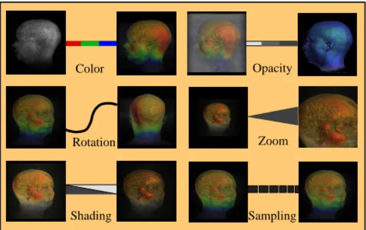
Figure 1: Edge representations for different rendering rameters. An edge represents the change in rendering pa-rameters between the two nodes it connects.

each newly rendered image is associated with ann-tuple of rendering parameters (color, opacity, zoom, rotation, light-ing, etc.). A notion of equality is defined for each of these rendering parameters. Two nodes on a graph are considered to be equal if all of their rendering parameters are equal. Two nodes are considered to be similar if all but one of their rendering parameters are equal. After each image is ren-dered, it is added to the graph. Then the node is attached to similar nodes in the graph. The similar nodes are con-nected with an edge that represents how they are related.

Because similar images can differ in one of several aspects, there are various types of edges that can exist between nodes. When a new node is added to the graph, at most one new edge of each type is drawn to prevent the graph from be-coming cluttered. Edges on the graph vary in appearance according to the type of relationship they represent. Figure 1 shows six different types. The reason for this distinction is to depict the changes made during the data exploration to get from one image on the graph to another. It is especially important to know the relationships between the images that have been rendered in case the types of the changes are not readily apparent from the images.

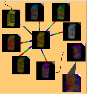
Figure 2 shows an image graph which provides the user with more information than just a group of images of the dataset. In particular, the graph makes it clear that first the user was experimenting with a variety of color maps. Next he produced images by changing the rotation of the desirable node, and then zoom factor. Note that nodes with similar parameters are close to each other in the graph even though they were not created in sequence. The mark on the top right corner of each thumbnail image indicates the rela-tive age of each node. Lighter marks correspond to the most recently created nodes. If these images are simply listed in the order of creation, it would be difficult to discern the relationships between these images just by looking at the im-ages themselves. A more complete description of the static representation, properties, and benefits of this graph-based approach is given in [11].

4

Graph-Based Rendering

Considering that the user’s task is essentially a search for desirable images within a space defined by the rendering pa-rameters, the image graph effectively represents user’s search pattern. For example, if after rendering an image using some

Figure 2: A graph representation of a set of images produced from the exploration of a dataset from a combustion engi-neering simulation of an industrial furnace. The goal was to reveal the temperature distribution inside the furnace. From this graph, one can see the user was first searching for an appropriate color transfer function before deriving the desir-able visualization shown in lower right image.

initial default parameters, the user wants to fine tune the ro-tation of the dataset to best display a certain small structure in the data, the user might render a series of images with differing rotations to search for the best rotation. This pro-cess would be represented on the graph as a group of images surrounding the initial image, with each of the surrounding images connected to the original image with a curved line, which is always used to represent a change in rotation. Once the user had found the correct rotation, he might continue his exploration by experimenting with different color and opacity values. Whatever images he rendered after finding the correct rotation would be attached to the image with the desired rotation. The graph would allow the user to quickly locate images of interest by looking at the relationship be-tween images. The graph allows the user to easily switch back and forth between different points in the image search space. A user could explore different rotations to make a structure visible as described above, and later try using dif-ferent opacity mappings to make the same structure visible independent of rotation. The user could switch back and forth between these approaches, and the graph would keep the nodes relating to the two approaches separate from each other.

This graph-based rendering can be much more dynamic. Once a few images are produced and added to the graph, the user can start manipulating the graph by editing the relationships between all of these images in the graph. The user can edit both nodes and edges in a graph. We describe the benefits of these features for data exploration in the rest of this section.

2

1

3

Figure 3: A portion of a graph representing the exploration of a foot dataset. Numbers were added to the graph for ease of illustration. The user combines the color and opacity maps of Node 1 in the top right corner with the zoom and rotation of Node 2 in the bottom left corner to produce Node 3 the image in the bottom right corner.

+

=

Figure 4: A desirable visualization result (right most) was produced using the union of two opacity transfer functions defined by the red and blue curves respectively. The left-most image (negative, blue vortices) corresponds to the blue curve. The middle image (positive, red vortices) corresponds to the red curve.

4.1 Editing Nodes

One feature the graph provides is the ability to combine the attributes of two existing nodes to produce a new node. During the process of searching for the rendering parame-ters which produce a useful image, a user may find several images which have some qualities of the desired image, but are not perfect. In this case, the user can drag one node on top of another node on the graph to produce an image which shares selected rendering parameters of the two par-ent nodes. Figure 3 prespar-ents an example. A dialog box lets the user specify which rendering parameters of each parent image will be used for the child image. The new image is then rendered and added to the graph, showing the relation-ship between the rendering parameters of the child and its parents.

The user can also generate some new rendering parame-ters using set operations such as union, difference and in-tersection. For example, an image may be generated based on an opacity transfer function which is the union of two others. Figure 4 presents an example in which the left-most

two images exhibit similar structures which in fact represent two different value ranges from the dataset. Here, scientists want to see both structures and their relationship in a single visualization, as can be produced with our union operation.

4.2 Editing Edges and Properties Propagation

Another method of editing the graph is manipulating edges to alter the changes in rendering parameters between two nodes. The user can select an edge on the image graph to bring up a dialog which allows the user to change the pa-rameter. Once the value of the parameter has been changed, the user can select a group of nodes to apply the change to. The user may apply the change to just one of the nodes di-rectly connected to the edge, or to all of the nodes on either side of the given edge. Using this method, a user can cause changes in rendering parameters to propagate through the graph. Specific property changes can either propagate for-ward (i.e. in the direction of the newer node attached to an edge), or backward according to the user’s wishes. This helps the user see the effects of a single parameter change as they exist in concert with many other combinations of parameters, all while keeping graph clutter to a minimum.

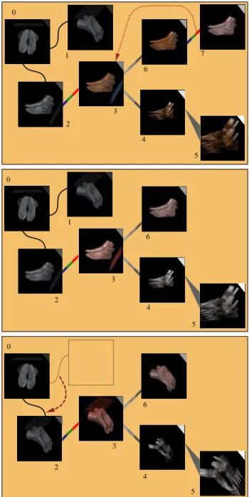
The user can also move edges within the graph, chang-ing its topology. When the user detaches one end of an edge from a node and attaches it to another, the parame-ter change associated with the edge is propagated through the new node and its peers. Using this approach, the user can apply a series of parameter changes to a group of nodes as a whole. Applying parameter changes in this way helps the user isolate the effects of various rendering parameters from each other in the images. This can help the user deter-mine which types of parameter changes cause which results in an image, as these effects are not always apparent from the images themselves. Figure 5 shows an example of the propagated effect before and after manipulating two edges. The consequence is the replacement of color transfer func-tion at Node 3, and the propagated effect throughout Nodes 4, 5 and 6. Node 7 is removed since it became redundant to Node 3. The second edge operation moves the top rotation edge over the bottom rotation edge. The propagation trig-gered allows the user to see all the visualization results on the right from a different view angle, the one Node 1 used.

Note that editing edges can result in a cyclic graph, in which case property propagation must be executed with care. Our current solution is to stop the propagation process when reaching an edge of the same type as the propagated property. In summary, the essence of the graph-based data exploration is that the user explore the data by creating a graph, operating on the graph, and reusing the same graph as much as possible.

4.3 Animation

Image graphs are also useful for making animation se-quences. The user selects from the graph the series of key-frame images to use for the production of the animation, and the system performs interpolation between them in the visualization parameter space to produce an animation. We use linear interpolation from the rendering parameters of one image to the rendering parameters of the next to pro-duce the intermediate images. Whether linear interpolation is appropriate or not for other types of visualization param-eters remains to be investigated.

Using this method the user can produce movies where, for example, the muscle tissue in a CT scan gradually fades

0 1 2 4 5 6 7 3 4 0 1 2 3 5 6 0 2 3 4 5 6

Figure 5: Top: an image graph produced from the foot dataset. A ”color” edge is being detached from node 7, and re-attached to node 3 in the graph. This action will replace the color transfer function of node 3 with the color map of node 7 and trigger a re-rendering at node 3. Furthermore, the effect of using a new color transfer function at node 3 will propagate through its peers. Middle: the resultant im-age graph after a forward propagation of a new property, in this case, the color transfer function. Compared to the images in the top graph, note that node 3, 4, 5, and 6 have all been updated. Node 7 has been removed since it has become redundant to node 3. Bottom: the resultant image graph after a forward propagation of a new property, in this case, rotation. Compared to the images in the middle graph, except the upper left image (Node 0), all other images are updated using the new viewing angle. Note that the user was able to create new visualization results without introducing new graph nodes.

Opacity Rotation Opacity Zoom

Figure 6: Making an animation using the image graph. Five key-frame were selected from an image graph to produce an animation sequence. From an image graph, the selection of key frame images becomes very intuitive to the user.

away to reveal only bone as the dataset is rotated. The main benefits of the image graph here are that the user can see the relationships between the images, and that images with similar properties are grouped together. So, when selecting the key frames for an animation the user can quickly find them with appropriate transitions, and have a rough idea of what the animation will look like before it is produced based on how the parameter changes affect the images in the graph. This intuitiveness of picking key-frame images would not be present with, say, a data flow network.

Figure 6 shows five key frames picked by a user, and Fig-ure 7 displays the selected frames from the resulting ani-mation produced by the system. In this example, between every two consecutive key-frame images, only one parame-ter is changed. In practice, change of multiple parameparame-ters between consecutive key-frame images may be desirable, in which case the interpolation for each parameter is done inde-pendent of other parameters, but their collective effect would show in the new images.

5

Graph Scalability and Displaying

The graph-based approach can become difficult to use after a great deal of images have been added to the graph. To address this issue, we have investigated several approaches to graph scalability. These approaches provide either a more detailed local view or a more compact global view of the original graph.

5.1 Local Views

Probably the simplest approach to solve the graph scalability problem is the use of a scrolled window. While a scrolled window is easy to implement, it only shows a subset of the graph - a very localized view of the overall graph. The user loses context. Thefisheye lens[4] is a mechanism for keeping the context while the user focuses on a smaller region. The distorted views of a large graph produced by using a fisheye len can be distracting.

A better approach to graph scalability involves providing both scrolling and zoom functionalities so that the user looks at a view of the graph which shows all of the nodes, or an enhanced view which displays a specific region of interest. In our current implementation the images representing the renderings of the dataset automatically scale in resolution as the zoom factor increases. This means that the user can get a very good look at an image on the graph by zooming in to it, without even having to load it into the main rendering window of our visualization system.

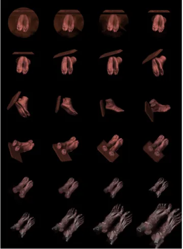
Figure 7: Selected frames from the resulting animation quence. The user can specify arbitrarily short or long se-quence between consecutive key frames.

5.2 Global Views

To keep the overall context, we first use a manual approach. The user can select nodes on the graph and collapse them. That is, remove them from the graph and store them else-where. These nodes can be added back to the graph later if the user wishes. In order to maintain correct graph topol-ogy in this case, the user is only allowed to collapse nodes with less than three edges active on the graph. However, if a user wishes to collapse a node with more than two edges, he can do this by collapsing surrounding nodes until the target node has the required number of edges, and then collapsing the node. When the user restores a node to the graph which has been collapsed, the node might not share an edge with any active node in the graph. To deal with this issue, the system computes the shortest path which connects the node to be added with the existing nodes, and adds the nodes and edges which form this path to the graph.

We have also implemented an automatic graph pruning approach, which involves using an least-recently-used algo-rithm to select nodes to remove from the graph when the number of nodes on the graph reaches a certain number. The user can mark certain nodes on the graph as immune from pruning, so that they will remain on the graph even if the user does not view or modify them for a long time. If a node is automatically pruned, it can be brought back into the graph just like manually pruned nodes.

5.3 Summary Graph

Another benefit the image graph approach provides for the user is the ability to view a summary graph which only shows the relationships between images that the user has marked as important. This functionality is useful in several scenarios. First, the user may wish to see the shortest path between the default rendering parameters and the parameters used for a desirable image. This functionality can be used to remove all nodes from the graph except those which lie on the path between nodes the user has marked as important. As well, the user may wish to show the relationship between a group of desirable images. In this case, the system can automatically remove all nodes from the graph which are not relevant to this relationship. This ability is especially important in the context of collaboration. A user who is unfamiliar with a dataset will find a graph which shows just the important images to be more useful than a graph which displays poor images produced during the data exploration process.

6

Collaborative Visualization

The exchange of image graphs among users is more useful than the exchange of just image data. Users can share, un-derstand, and build upon each others results. If a group of images is used, the user has no clear idea of the relationship between them. If users want to work together to explore a dataset, it is important to minimize the amount of a user’s work which is lost when that work is communicated to an-other user. By expressing the data exploration process in terms of an image graph as opposed to a list of images, the system can communicate more information to other users. When a user explores a new dataset, the first step is to lo-cate a reasonable set of rendering parameters which produce an intelligible image. Once this starting point is reached, the user can begin to refine the image. During this process of re-finement, a lot of information about the dataset is discovered which can not be captured by images alone. The user may learn, for example, that for a given dataset changes in the color map do little to change the resultant image compared to the change caused by changes in the opacity map. In a collaborative scenario, it is useful to communicate this infor-mation to other users so they would not have to rediscover it. The image graph accomplishes this goal.

Moreover, this sharing becomes more effective with anno-tated image graphs. Annotation is done by drawing on the actual images, or by writing comments about the images. These comments are stored in the visualization graph along with the nodes to which they correspond. As well, these graphs can be saved for later use. The annotated graphs can then be exchanged among users of the system. Figure 8 shows an annotated image.

7

System Architecture

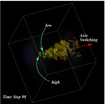
We have implemented a web-based volume visualization sys-tem which includes all of the image graph features described in this paper. The main components of our system are the render server, the communication server, and clients. Fig-ure 9 presents the system architectFig-ure of the testbed. In this section each of these components is discussed in further detail. low high Axis Switching Time Step 98

Figure 8: Visualization of data from modeling of turbulent jet flow. The image is annotated by a user to point out features showing low and high pressure, and the axis-switch property of the flow.

7.1 Render Server

The render server is the process which actually performs the rendering of the image to be displayed on the client. This server is started by the proxy server when needed in order to fulfill a rendering request from a client. Because the system is modular, different implementations of the render server can be used interchangeably. The current implementation uses both the shear warp algorithm [7] and a ray casting al-gorithm [9] to render data on Cartesian grids. The system selects which algorithm to use based on the size of the im-age requested and our performance data. With our current configuration, the ray casting algorithm performs better on smaller images and the shear warp algorithm performs bet-ter on larger images. In addition, the ray casting algorithm is used to render zoomed images as the shear warp imple-mentation does not support supersampling.

Both rendering algorithms can benefit from preprocessing. To speed up subsequent rendering calculations, the shear warp algorithm as used in our system uses two stages of pre-processing: classification and octree encoding. Octree en-coding is dependent on the opacity transfer function used. This means that if the render server’s preprocessing is up to date, a new image of the dataset can be rendered very quickly if only the color transfer function or the view trans-formation is changed. On the other hand, the ray casting renderer uses a view-dependent ray cache to achieve very fast rendering rates independent of changes of transfer functions.

7.2 Proxy Server

The proxy server handles the communication of the clients and the render server. It provides mechanisms for access control, tracking the state of a client’s session, load balanc-ing, and caching. When a client is started, it connects to the proxy server. The server can choose to allow the client to

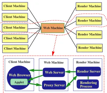
Applet

Web Browser Web Server Proxy Server

Render Server

Rendering Process Client Machine Web Machine Render Machine

Render Machine Render Machine Render Machine Render Machine Client Machine Client Machine Client Machine Clinet Machine Clinet Machine Web Machine

Figure 9: System Architecture of the testbed.

connect or not, based on any desired set of rules. For exam-ple, the proxy server might want to limit access to only ten users at a time. The server could also only accept connec-tions from within a certain network, or according to some other metric.

If a client is allowed to connect, the server begins keeping track of the rendering parameters associated with the cur-rent client session. A separate set of rendering parameters is maintained for each client connected, so that many clients can connect at a time. A single proxy server can also connect to a variety of render servers. This allows a proxy server to distribute a rendering load by assigning separate rendering tasks to rendering processes running on different machines. While our current implementation does not support the di-vision of the task of rendering a single image among multiple servers, this type of separation is a possibility for future ex-ploration.

The proxy server also implements a caching mechanism to try to reduce the number of images that need to be rendered. When an image is generated, the rendering parameters used to generate that image are stored along with the image. If another image is requested later using the same rendering parameters, the initial image is used.

The shear warp algorithm can take advantage of pre-processing in order to reduce rendering time. The proxy server determines what type of preprocessing to do based on changes in the state of the clients. As new images are produced, the proxy server tells the render server to do the correct preprocessing.

7.3 Client

The Java client displays a user interface for the system. The interface allows the user to upload data, filter the data, set and adjust rendering parameters, displays the images pro-duced by the render server, and organizes a concise history of the visualization process conducted by a user. We have been experimenting with different user interface designs for this volume visualization system. The Java client will allow us to conduct user studies of our designs by using users at remote sites.

8

Conclusions

Image graphs help streamline the process of visual data ex-ploration in two ways. First, the graphs give the user a representation of the relationship between visualization pa-rameter changes and the images produced using them. As we have pointed out in an example using volume rendering, often these relationships are not obvious just through in-spection of the rendered images. An understanding of how specific rendering parameter changes will affect the image output is important because it reduces the number of im-ages the user must produce to find parameters which yield a useful image, and these images can be quite time consuming to produce.

Second, the dynamic features of the graphs, such as an-notation and automatic pruning, facilitate collaboration and animation. They also help speed the search for good ren-dering parameters by allowing users to perform operations on groups of nodes. These operations include simple mod-ification of rendering parameters, combination of nodes to form ”child” nodes with their properties, and propagation of modifications through the graph.

The results of an informal user study we have conducted using twelve resident staff scientists indicate that image graphs reduce the average amount of time needed to come up with desirable images of complex volumetric datasets. We are presently designing a comprehensive user study to refine the design of the visualization system and its image graph interface. We are particularly interested in learning to what extent that image graphs may be reused.

While the examples in this paper relate to volume render-ing, we think image graphs would be useful for any type of data exploration problem which produces images of data as a function of some set of parameters. Other possible applica-tions include radiosity calculaapplica-tions, 2-D image filtering, and polygon based rendering. Our future work, thus, includes demonstrating that our approach is indeed useful for these other problem domains.

Acknowledgements

This research was supported by the National Aeronau-tics and Space Administration under NASA Contract Nos. NAS1-19480 and NAS1-97046 while the author was in resi-dence at the Institute for Computer Applications in Science and Engineering (ICASE), NASA Langley Research Center, Hampton, VA 23681-2199. James Patten, an undergraduate student at University of Virginia, with excellent program-ming skill implemented a prototype of the image graphs de-sign while he spent two summers at ICASE. The foot data set was extracted from the the Visible Woman data set. The furnace data set was provided by Dr. Philip Smith at Uni-versity of Utah, and the turbulent flow data set was provided by Dr. A. O. Demuren at Old Dominion University.

References

[1] G. Abram and L. Treinish. An extended data-flow architecture for data analysis and visualization. In Proceedings of the IEEE Visualization ’95 Conference, pages 263–270, October 1995.

[2] G. Collaud, J. Dill, P. Tan, and C. V. Jones. CZWeb: Fish-eye views for visualizing the world-wide web. In

Proceedings of the HCI International ’97: the 7th Inter-national Conference on Human-Computer Interaction, August 1997.

[3] T. T. Elvins, D. R. Nadeau, and D. Kirsh. Worldlets -3d thumbnails for wayfinding in virtual environments. InProceedings of the ACM Symposium on User Inter-face Software and Technology, pages 21–30, October 1997.

[4] G. W. Furnas. Generalized fisheye views. InHuman Factors in Computing Systems, CHI ’86 Proceedings, pages 16–23, April 1986.

[5] T. He, L. Hong, A. Kaufman, and H. Pfister. Gener-ation of transfer functions with stochastic search tech-niques. InProceedings of Visualization ’96, pages 227– 234, October 1996.

[6] G. Kindlmann and J. W. Durkin. Semi-automatic gen-eration of transfer functions for direct volume render-ing. InProceedings of 1998 Symposium on Volume Vi-sualization, pages 79–86, October 1998.

[7] P. Lacroute and M. Levoy. Fast Volume Rendering Us-ing a Shear-Warp Factorization of the ViewUs-ing Trans-formation. In Proceedings of SIGGRAPH ’94, pages 451–458, July 1994.

[8] M. Levoy. Spreadsheets for images. InProceedings of SIGGRAPH ’94, pages 139–146, July 1994.

[9] K.-L. Ma, M. F. Cohen, and J. S. Painter. Volume Seeds: A Volume Exploration Technique. The Journal of Visualization and Computer Animation, 2:135–140, 1991.

[10] J. Marks, B. Andalman, P. Beardsley, W. Freeman, S. Gibson, J. Hodings, T. Kang, B. Mirtich, H. Pfister, W. Ruml, K. Ryall, J. Seims, and S. Shieber. Design Galleries: A general approach to setting parameters for computer graphics and animation. In Proceedings of SIGGRAPH ’97, pages 389–400, August 1997.

[11] J. Patten and K.-L. Ma. A graph based interface for rep-resenting volume visualization results. InProceedings of Graphics Interface ’98, pages 117–124, June 1998. [12] C. Upson, T. Faulhaber, D. Kamins, D. Schlegel,

D. Laidlaw, J. Vroom, R. Gurwitz, and A. van Dam. The application visualization system: A computational environment for scientific visualization. IEEE Com-puter Graphics and Applications, 9(4):30–42, 1989. [13] D. Young, M. Argiro. Cantata: Visual programming

environment for the khoros system. Computer Graph-ics, 29(2):22–24, May 1995.