Integer Programming Formulations for the
Uncapacitated Vehicle Routing p-Hub Center Problem
Z. Kartalaand A.T. ErnstbaAnadolu University, Department of Industrial Engineering, 26555, Eskisehir, Turkey bCSIRO, Private Bag 33, Clayton South, Vic. 3169, Australia
Email: [email protected]
Abstract: Hub facilities are used in many-to-many transportation networks such as passenger airlines,
parcel delivery,andtelecommunication systemnetworks. In thesenetworks, the flow that isinterchanged
betweenthedemandcentersisroutedviathehubstoprovidediscountedtransport.Manyparceldeliveryfirms
serveonahub basedsystem where the flows from different demand nodes are concentrated, sorted and
disseminated at the hubcenters inorderto transferthem tothe destinations points. The main purpose of
hub location problemis todecide the locationof hub facilities andtoallocate demand nodesto thehubs.
In hub based systems, as analternative way of serving each origin destinationnode directly, the flow is
accumulatedatthehubfacilitiesinordertoexploitthesubstantialeconomiesofscale.
Hub location problems can be categorized in terms of the objective function of the mathematical models. In the literature, hub location problems with total transportation cost objectives (median), min-max type objectives (center) and covering type objectives are well studied.
In the hub location problem literature, it is assumed that only one vehicle serves between each demand center and hub. The vehicles are not permitted to visit more than one city. The need to design a network of combined hub locations and vehicle routes arises in various applications. For example, in cargo delivery systems, sending separate vehicles between each demand center and hub is rather costly in terms of investment on the total number of vehicles. Instead, if the vehicles are allowed to follow a route by visiting different demand nodes in each stop, the total investment cost may decrease considerably. In airline companies, similarly, if a separate aircraft and separate air staff are assigned for each destination, they incur high investment and operating costs. Also, traffic congestion occurs at airports and in air networks.
In the light of above-mentioned real life considerations, the vehicle routing hub location problem has been receiving increased attention from researchers. This problem is to decide the location of hubs, the allocation demand centers to the hubs and the associated routing structure with multiple stopovers and allowing vehicles to make a tour so as to minimize total transportation cost.
In addition to the cost, parallel to the increase of the competition in the market, companies tend to promise to the customers ’next day delivery’ or ’delivery within 24 h’ guarantees. However, the hub location and vehicle routing problem, which consider both the flows and distances, may sometimes lead to delays from non-simultaneous arrivals at hubs, when worst-case route lengths for vehicles are excessively large. Although classical hub location problems provide one option when origin-destination distances are huge, they become less appropriate when vehicle routing is required and delivery time is a major concern.
In this study, we introduce the uncapacitated vehicle routingp−hub center problem to the literature. The
aim of our model is to find the location of the hubs, assign demand centers to the hubs and determine the routes of vehicles for each hub such that the maximum distance or travel time between origin-destination pairs
is minimized. We propose mathematical programming formulations for this problem with O (n2) and O (n4)
variables. The formulations trade off tightness against formulation size. The computational results on standard data sets from the literature allow this trade off to be evaluated empirically and provide an indication of the challenge of solving these combined vehicle routing hub location problems.
Keywords:p-hub center problems, hub location, hub location and routing problem,p-hub center and routing problems
1 INTRODUCTION
In most many-to-many distribution systems, goods are collected from various origins to be distributed to various destinations. However, sending the goods directly from each origin to each destination with a dedicated vehicle is often not economical, since the flow rates for a substantial fraction of the origin-destination pairs can sometimes be so small. Hub network systems are used to consolidate the flows between origin-destination pairs to eliminate expensive direct connection.
The aim of the classical single allocationp-hub median problem is to minimize the total cost of transportation
while establishingpnodes (hubs) among a given set of nodes with pairwise traffic demands and allocate each
non-hub node to the hubs. While in thep-hub center problem, the main objective is minimizing the maximum
distance/cost between origin-destination pairs. In the hub location problems, the flow fromi toj must be
routed on at least one hub if both the nodesiandjare allocated the same hub; otherwise at most two hubs, if
nodeiandjare allocated to different hubs. There is a path in the route asi−k−l−jif nodeiis allocated to
hubkand nodejis allocated to hubl. The flow traversing the hub linkk−lis the flow from nodes allocated
to hubkto nodes allocated to hubl. Commonly a discount factor applies on the inter-hub connections since
the transportation cost on these links are lower due to economies of scale. Surveys on various different hub location problems can be found in Campbell and O’Kelly [2012] and Alumur and Kara [2008].
The fundamental assumption of hub location problem is that there is a direct connection between each non-hub node and its assigned hub. However, more recently, this unrealistic assumption have been adjusted and adapted to deal with some transportation problems and logistics applications in hub networks where nodes do not have adequate demand to connect them directly with hubs [Rodriguez-Martin et al., 2014].
In this paper, we introduce the uncapacitated vehicle routing p-hub center problem (UVRpHCP) to the
lit-erature, relaxing the main hub location problem assumption, where there is a separate vehicle which serves between any non-hub node and its assigned hub. To the best of authors’ knowledge, no previous study has
investigated the combination of p-hub center and vehicle routing problems. The aim of the problem is to
minimize maximum distance/cost between any origin-destination pair, while locatingphubs, assigning the
non-hub nodes to exactly one hub and forming the routing structures of the given vehicles for each hub. The outline of the paper is as follows. In the next section, we introduce three different mathematical
formula-tions of the UVRpHCP, whose complexities in terms of variables are O (n2) and O (n4). In the third section,
we give some numerical tests with regard to all formulations. Finally, in the last section concluding remarks are presented.
2 MATHEMATICALFORMULATIONS
The UVRpHCP determines the location of the hubs, the allocation of non-hub nodes to hubs, and the associ-ated routing structure between non-hub nodes and hubs with multiple stopovers so as to minimize maximum distance/cost between origin-destination pairs. This problem can be defined on a complete, symmetric
net-work;G= (N, A)with node setN ={1,2, ..., n}and arc setA. Each arc(i, j)∈N has a nonnegative cost
(distance),dij =djisatisfying the triangle inequality. The economy of scale is modeled by a discount factor
α∈(0,1)between hub nodes. The costs can be used to capture travel time, path length or monetary costs.
We assume that a limited fleet of homogenous uncapacitated vehicles v ∈ V operates on the routes. The
number of available vehicles for each hub to deploy; n(i)is known a priori. These vehicles should visit at
least two nodes including the hub itself, also they are allowed to visit multiple non-hub nodes. There is no upper bound on the number of nodes that a vehicle can visit. It is also assumed that larger sized and faster vehicles operate between two hubs. It is not permitted for these vehicles make any additional stops along their trips.
One of the main difficulties for solving hub location problems is to deal with larger numbers of variables and constraints in the formulations. Therefore, formulations with fewer variables and constraints have been devel-oped. However, although the larger formulations lead to tighter lower bounds, increased computational times are also required to find and exact solution. For this reason, we first explored an integer linear programming
model with O (n4) variables to solve UVRpHCP. The motivation behind our first model, which is based on a
classical four-index hub location formulation, is to get tighter lower bounds associated with the LP relaxation.
To formulate the problem, we use the idea of the Campbell [1994] study, in whichyijklis defined as the fraction
of flow; as being 1 if a vehicle is taking mail originating at nodeiand destined for nodejalong the road from
that whileyklij andfklij variables are allowed to be fractional in the formulation, they are always integer in the
optimal solution corresponding to the shortest path from nodeiandjin the hub network. In this formulation,
the path followed by vehicles is defined in the model using the variables xv
ij which take on the value 1 if
vehiclevvisits nodei∈N and nodej ∈N \ {i}in a route, and 0 otherwise. In the suggested formulation,
there is a three indexedxvijvariable for every arc-vehicle combination.
Lethito be a zero-one variable withhi= 1 if nodei∈Nis a hub and 0 otherwise. Integer variableziv∈ {0,1}
to denote if vehiclev∈V is assigned to hubi∈N (ziv=1) or not (ziv=0).
The mathematical programming formulation of the UVRpHCP with four-indexed flow variables is as follows: Model-1 min Z1, (1) s.t. X k X l dkly ij kl+ X k X l α dklf ij kl ≤Z1, ∀i, j (2) fklij = flkji, ∀i, j6=i, k, l6=k, (3) X k6=i (yijik+ fikij) = 1, ∀i, j6=i, (4) X l6=k,l6=i (ylkij+ flkij)− X l6=k,l6=i (yklij+ fklij) = 1, ∀i, j6=i, k6=i, k=j, (5) yijkl≤X v xvkl, ∀i, j6=i, k, l6=i, (6) X l (fklij+ flkij)≤ hk, ∀i, j, k∈N, (7) X i hi=p, (8) X j6=i xvij−X j6=i xvji= 0, ∀i, v (9) X v ziv =hini, ∀i (10) ziv ≤ X j6=i xvij, ∀i, v (11) X v X j6=i xvij =X v ziv+ (1−hi), ∀i (12) X j6=i xvij−1 +hi≤ziv, ∀i, v (13) X i ziv = 1, ∀v (14) ziv, xvij, hi∈ {0,1} ∀i, j∈N, v∈V (15) 0≤fklij, yijkl≤1 ∀i, j, k, l∈N, (16) The objective function (1) minimizes the maximum distance/cost. The first term in (2) calculates total dis-tance/cost for a route. The second term calculates the total distance between two hubs. Constraint (3) ensures
that the fraction of flow that travels from nodeito nodejvia hubs located atkandlis equal to the fraction
of flow that follows a route from nodeito nodejvia hubslandk. Constraint (4) guarantees that total flow
fromitojis transferred. Constraint (5) is the flow conservation constraint. Constraint (6) defines the amount
of vehicle flow originated at nodeidestined toj uses the link(j, k)from nodej to nodek. Constraint (7)
ensures that the total flow is transferred via hubkand hubl. Constraint (8) ensures that exactlyphubs are
to be located. Constraint (9) is known as degree constraint. With this constraint it is guaranteed that every
node has as many vehicles arriving as leaving. If nodeiis hub, the number of assigned vehicles for this hub
isn(i), which is ensured by constraint (10). If nodeiis hub, the arc between hub nodeiand non-hub nodej
is served with exactly one vehicle which is guaranteed by constraint (11). Constraint (12) states that if nodei
hand, if nodeiis not a hub, then this constraint guarantees that eachi−jnon-hub link is visited only once by
a vehicle. By constraint (13),zivtakes value only if nodeiis a hub node. With constraint (14) it is guaranteed
that each vehicle is only allocated to one hub.
This model has (n2v+nv+n) binary variables, (2n4) positive variables and (2n4+ 2n3+ 2n2+ 3nv+ 2n+v)
constraints. Thus, there are O (n4) variables and O (n4) constraints in total.
Secondly, we explored a three index vehicle flow formulation which uses substantially fewer variables than our
O (n4) formulation. Therefore, we hope to solve much larger problems with our new formulation which has
O (n2) variables. Using the same notation as for the four index hub location formulation, we define additional
decision variables and parameters;
aij :1, if nodejis the successor node of non-hub nodei; 0 otherwise.
bw
ij:1, if vehiclewtravels from nodeito nodej; 0 otherwise.
abv
ij:1, if vehiclevtravels from nodeito nodej, and nodeiis not a hub; 0 otherwise.
transf ervw:the distance between two hub nodes.
collectv :the longest collection distance from any location served by vehiclevto the hub.
distribw:the longest distribution distance to any location served by vehiclew.
L:the maximum number of nodes a vehicle may visit.
ui:auxiliary variable - defines distance to the hub for subtour elimination.
The second mathematical formulation that we developed for UVRpHCP uses O (n2v) variables. Note that
sincev is typically very small, this formulation is not significantly larger than the third model with O (n2)
variables. Model-2 min Z2, (17) subject to: (8)−(15) X j aij = 1, ∀i (18) aij ≤ 1−hi, ∀i, j (19) aij ≤ X v xvij, ∀i, j (20) aij ≥ xvij−hi, ∀i, j, v (21) ui−uj+L∗aij ≤ L−1, ∀i, j (22) X j X w bwij = 1, ∀i (23) bwij ≥ xwij−hj, ∀i, j, w (24) X i X j6=i (bwijdij) =distribw, ∀w (25) X j X v abvij = 1, ∀i (26) abvij ≥ xvij−hi, ∀i, j, v (27) X i X j6=i (abvijdij) =collectv, ∀v (28) X j dijzjw−max j {dij}(1−ziv)≤transf ervw, ∀i, v, w (29) X i X j6=i dijxvij−dklxvkl−M(1−x v kl)≤collectv+distribv, ∀k, l, v (30)
collectv+distribw+α×transf ervw≤Z2, ∀v6=w (31)
aij, bvij, ab v
ij ∈ {0,1} ∀i, j∈N, v∈V (32)
The objective function (17) minimizes the maximum distance/cost. This cost includes the total distance be-tween hubs, plus the distance beginning from the first non-hub node in a vehicle route to the hub (collection) and lastly the distance/cost from the last non-hub node in a vehicle route to the hub (distribution). Since the
single allocation scheme is used, each non-hub nodeiis visited only once which is guaranteed by constraint
(18). Constraint (19) ensures that if nodeiis a hub node,aij takes on value 0. On the contrary, if nodeiis
not a hub node, then there should be a link between nodeiand nodej. If nodeiis not a hub node and node
j is a hub node, then constraint (20) limits the number of entering arcs into the hub nodej to the number
of available vehicles. By constraint (21)aij is one ifiis a non-hub node and arci−j is visited by exactly
one vehicle. Constraints (22) are sub-tour elimination constraints. Constraints (23)–(25) together calculate the maximum distribution cost/distance amongst all vehicles. Similarly, constraints (26)–(28) together cal-culate the maximum collection cost/distance amongst all vehicles. Constraint (29) calcal-culates the maximum cost/distance amongst all hub pairs. When constraint (30) is active the maximum distance is determined by
two successive nodes on the route of vehiclev, that is we are calculating the distance fromlto the hub and then
from the hub to nodekwhere arc(k, l)is on the route ofv. Lastly, constraint (31) ensures that the objective is
no less than the travel distance/cost between any pair of nodes allocated to the vehiclewandv, sincecollectv
anddistribwgive the longest distances of vehiclevandwfor different hubs, respectively.
Model-2 for UVRpHCP is a mixed integer program that has (3n2v+n2+nv+n) binary variables, (n+v2+2v)
positive variables and (n2v2+ 3n2v+ 3n2+nv2+v2+ 3nv+ 5n+ 3v) constraints. Thus, there are O (n2v)
variables and O (n2v2) constraints in total.
Finally, we describe a third formulation which is based on a two-index vehicle flow formulation that uses O
(n2) binary variables, that keeps every arc; for the determination path of the vehicle routes. In this formulation,
the path followed by vehicles are defined in the model by means ofxij variables which takes on the value 1 if
nodei∈N precedes nodej ∈N\ {i}and 0 otherwise. Integer variablessiv ∈ {0,1}is used to represent
if nodei ∈ N is serviced by vehiclev ∈ V (siv = 1) or not (siv = 0). Following the idea ofp-hub center
formulation in Ernst et al. [2009], which is based on the concept of a hub radius, the other variables arer1
ivthe
total distance from the first non-hub node to hub nodeiin a vehicle routev; similarly,r2
ivthe total distance
from the hub nodeito last node in a vehicle routev. And lastly, in order to calculate the distances of two
different vehicles for the same hub, we definerv1
ivto be the total distance from the first non-hub node to hub
nodeiin a vehicle routev;rv2
ivdenotes the the total distance from the hub node ito last node in a vehicle
routev. The third formulation which has O (n2) binary variables with two index vehicle flow formulation is
then given below:
Model-3 min Z3, (34) subject to: (8),(14) X j6=i xij− X j6=i xji= 0, ∀i (35) X j xij= 1 + (ni−1)hi, ∀i (36) X v siv= 1 + (ni−1)hi, ∀i (37) X i siv≥2, ∀v (38) ziv≤hi, ∀i, v (39) ziv≤siv, ∀i, v (40) ziv≥hi+siv−1, ∀i, v (41) siv≥sjv+xij−1−hj, ∀i, j, v (42) siv≥sjv+xji−1−hj, ∀i, j, v (43) r1iv≥r1jv+dij−M (1−xji)−M hj−M (1−siv), ∀i, j, v (44) r2iv≥r2jv+dij−M (1−xij)−M hj−M (1−siv), ∀i, j, v (45) rv1iv≥rv 1 jv+dij−M (1−xij)−M hi−M (1−siv), ∀i, j, v (46)
rv2iv≥rv2jv+dij−M (1−xij)−M hi−M (1−siv), ∀i, j, v (47) Z3≥r1iv+α dij+r2jw−M (1−hi)−M (1−hj) ∀i, j, v, w (48) Z3≥ rviv1 +rv 2 jv−M (1−xij) ∀i, j, v (49) xij, siv, hi∈ {0,1} ∀i, j, v (50) r1iv, rjv2 , rv1iv, rviv2 ≥0, ∀i, j, v, (51) The objective function (34) minimizes maximum distance between hubs, plus the distance beginning from the first hub node in a vehicle route to the hub (collection) and lastly the distance/cost from the last non-hub node in a vehicle route to the non-hub (distribution). Constraint (35) is known as the degree constraint. By
constraints (36) it is guaranteed that if nodeiis a hub, the number of arcs that leave from nodeiis equal to
the number of assigned vehicles. On the other hand, if nodeiis not a hub, then these constraints guarantee
that eachi−jnon-hub link is visited only once. Constraint (37) guarantees that each non-hub link is visited
by only one vehicle unless node i is not a hub node. Constraint (38) guarantees that for any vehicle the
number of visited nodes including hub node itself is greater than or equal to two. With constraint (39) it is guaranteed that each vehicle is only allocated to one hub. By constraint (40) no vehicle is assigned to a node unless a hub is opened at that site. Constraint (41) allows assigning a vehicle to a hub node. Constraints
(42) and (43) together guarantee that if there is a link between node iand nodej, both of these nodes are
visited by the same vehicle. Constraint (44) keeps the longest distance for a vehicle from the first non-hub node to hub node in the route (collection) where M is a large number. Similarly, constraint (45) keeps the longest distance/cost for a vehicle from the hub to the last node of the route (distribution). Constraint (46) calculates the longest collection distance/cost between two nodes in a vehicle route. Constraint (47) calculates the longest distribution distance/cost between two nodes in a vehicle route. If the collection plus distribution cost/distance for two vehicles’ of one hub is greater than the two different vehicles of different hubs plus the cost/distance between the hubs, constraint (49) allows that the objective function value must be greater than this value. Notice also here that due to constraints (44), (45), (46) and (47) sub-tours are eliminated. For
solvingModel-1, M is taken as the longest distance times number of nodes in the data set.
This mathematical model has (n2+ 4nv+n) binary variables, (4nv) positive variables and (n2v2+ 7n2v+
3nv+ 3n+ 2v) constraints. Thus, there are O (n2) variables and constraints in total.
3 COMPUTATIONALRESULTS
In this section we present the results with regard to the three formulations that are described in this paper. We solved these using GAMS 23.8 with the GUROBI 4.6 solver on a 64 bit Intel i5 (3.30 Ghz) machine with 8 GB RAM. The effectiveness of our mathematical models were tested on the Civil Aeronautics Board (CAB) data set. This data set, introduced in O’Kelly [1987], is derived from airline passenger data between 25 US cities
that includes demands and distances. In order to provide results, we tookn= 10andn= 15nodes problem
instances with different numbers of vehicles and hubs. While solving the mathematical models, we limited the CPU time to two hours on GAMS. We report the results from GUROBI performance measures in Table 1.
For each instance in Table 1, the first column gives the characteristics of the test problemn.p.vwherenis the
number of nodes,pis the number of hubs andvis the number of vehicles that are assigned for each hub. In
each instance we setα= 1. The second column gives the optimal solution. In the instances when any of the
mathematical models could not find the optimal solution, reported with an asterisk (*) in the second column, we give the best integer solution found with one of the mathematical models. The rest of the table has three
main parts. We give the same performance measures reported by GUROBI for O (n4) variable formulation, O
(n2) variable with three index vehicle flow formulation, and lastly O (n2) variable with two index vehicle flow
formulation, referred to asModel-1,Model-2andModel-3, respectively. In the three columns for three models,
we first provide the number of nodes in the branch and bound tree, the CPU time requirement in seconds and
gap i.e.,ubub−lb∗100as reported by GUROBI, wherelbis the final lower bound andubis the final upper bound.
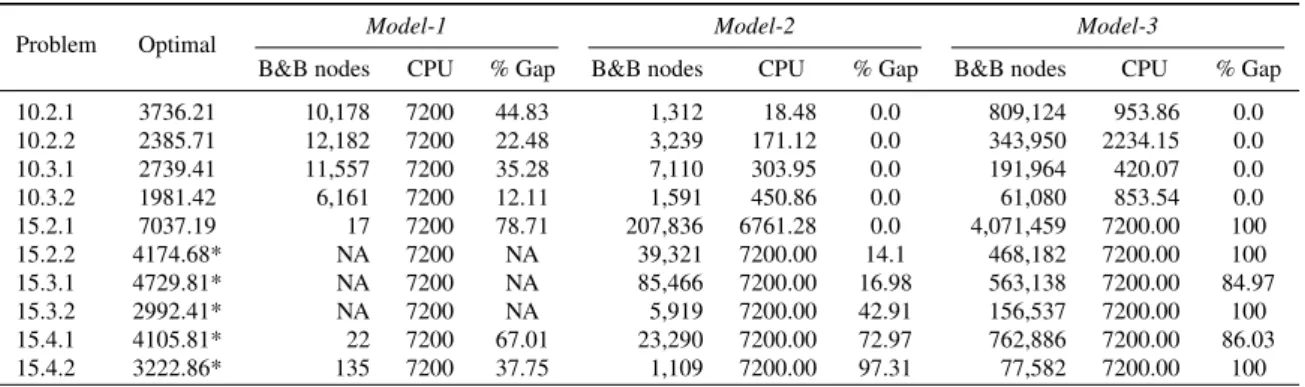
Observe from Table 1 that,Model-2andModel-3solved all the instances with 10 nodes optimally in less than
one hour of CPU time. Model-2also solved 15.2.1 to optimality within two hours. We remark here that, the
lowest objective values amongst three mathematical models is found byModel-2.
We also observe that Model-1 has the tightest LP relaxation over all the problem instances, although LP
relaxation values are still far from the optimal upper bound.The reason is that theO(n4)variable formulation
is the strongest formulation of the three models. However, this tightness comes at the cost of greatly increased computational time. Using this formulation, no optimal solution found within two hours. We note here that
Table 1. Results for Models on CAB data sets
Problem Optimal Model-1 Model-2 Model-3
B&B nodes CPU % Gap B&B nodes CPU % Gap B&B nodes CPU % Gap 10.2.1 3736.21 10,178 7200 44.83 1,312 18.48 0.0 809,124 953.86 0.0 10.2.2 2385.71 12,182 7200 22.48 3,239 171.12 0.0 343,950 2234.15 0.0 10.3.1 2739.41 11,557 7200 35.28 7,110 303.95 0.0 191,964 420.07 0.0 10.3.2 1981.42 6,161 7200 12.11 1,591 450.86 0.0 61,080 853.54 0.0 15.2.1 7037.19 17 7200 78.71 207,836 6761.28 0.0 4,071,459 7200.00 100 15.2.2 4174.68* NA 7200 NA 39,321 7200.00 14.1 468,182 7200.00 100 15.3.1 4729.81* NA 7200 NA 85,466 7200.00 16.98 563,138 7200.00 84.97 15.3.2 2992.41* NA 7200 NA 5,919 7200.00 42.91 156,537 7200.00 100 15.4.1 4105.81* 22 7200 67.01 23,290 7200.00 72.97 762,886 7200.00 86.03 15.4.2 3222.86* 135 7200 37.75 1,109 7200.00 97.31 77,582 7200.00 100
the LP relaxation yielded byModel-1is always the longest distance in the data set we considered. However,
the LP relaxation value of O (n2) variable models are always zero, except in the first problem instance for
Model-2.
Lastly, we remark here that the O (n2) model with two index vehicle flow formulation has the largest branch
and bound tree to be explored compared to other models. We also note here that althoughModel-3is based on
the most successful formulation in terms of the solution time in the literature for the standard single allocation p-hub center problem, the performance of it is weak on the uncapacitated vehicle routingp-hub center problem.
Clearly, the O (n2v) model with three index vehicle flow formulation is superior toModel-1andModel-3in
terms of the solution quality achieved in reasonable amounts of CPU time. 4 CONCLUSIONS
In this paper we studied a new hub location problem UVRpHCP. To the best of the authors’ knowledge, ours is the first study in the literature that combines vehicle routing and the p-hub center problem. To solve this
problem we developed three integer programming models ranging in size formO(n2)toO(n4)variables.
We tested the performances of the formulations on the well-known CAB data set. The numerical results
showed the formulation Model-2 with O (n2v) variables (wherenis the number of nodes andvthe number of
vehicles) is superior to the other formulations in terms of computational time and solution quality.
Real world problems are, unfortunately, significantly larger than any solved exactly in this paper. Therefore, future work must focus on solving larger problems. This could be achieved by developing new mathematical models that reduce symmetry. For example in all of our formulations renumbering the vehicles leads to equiv-alent (symmetric) solutions. Reducing such symmetry is likely to have a positive impact but more significant algorithmic improvements are expected to be necessary to obtain exact solutions to medium and large sized instances.
REFERENCES
Alumur, S. and B. Kara (2008). Network hub location problems: The state of the art. European Journal of
Operational Research 190(1), 1 – 21.
Campbell, J. (1994). Integer programming formulations of discrete hub location problems.European Journal
of Operational Research 72(2), 387 – 405.
Campbell, J. F. and M. O’Kelly (2012). Twenty-five years of hub location research. Transportation
Sci-ence 46(2), 153–169.
Ernst, A. T., H. Hamacher, H. Jiang, M. Krishnamoorthy, and G. Woeginger (2009). Uncapacitated single and
multiple allocation p-hub center problems. Computers & Operations Research 36(7), 2230–2241.
O’Kelly, M. (1987). A quadratic integer program for the location of interacting hub facilities. European
Journal of Operational Research 32(3), 393 – 404.
Rodriguez-Martin, I., J.-J. Salazar-Gonzalez, and H. Yaman (2014). A branch-and-cut algorithm for the hub