A Novel Rule Induction Algorithm with Improved
Handling of Continuous Valued Attributes
A thesis submitted to the Cardiff University For the degree of
Doctor of Philosophy
By
Dinh Trung Pham
School of Engineering, Cardiff University United Kingdom
Abstract
Machine learning programs can automatically learn to recognise complex patterns and make intelligent decisions based on data. Machine learning has become a powerful tool for data mining. A great deal of research in machine learning has focused on concept learning or classification learning. Among the various machine learning approaches that have been developed for classification, inductive learning from examples is the most commonly adopted in real-life applications.
Due to non-uniform data formats and huge volume of data, it is a challenge for scientists across different disciplines to optimise the process of knowledge acquisition from data with naïve inductive learning techniques. The overarching purpose of this research is to develop a novel and efficient rule induction algorithm a learning algorithm for inducing general rules from specific examples that can deal with both discrete and continuous variables without the need for data pre-processing.
This thesis presents a novel rule induction algorithm known as RULES-8 which utilises guidelines for the selection of seed examples, together with a simple method to form rules. The research also aims to improve current pruning methods for handling noisy examples. Another major concern of the work is designing a new heuristic for controlling the rule formation and selection processes. Finally, it concentrates on developing a new efficient learning algorithm for continuous output using fuzzy logic theory. The proposed algorithm allows automatic creation of membership functions and produces accurate as well as compact fuzzy sets.
Acknowledgements
This thesis would not have been accomplished without the guidance and support of a great number of people to whom I would like to convey my utmost gratitude.
My first and most special thanks go to Professor D. T. Pham for his supervision, guidance and advice from the early stage of my studies at previous MEC – Manufacturing Engineering Central of Cardiff University. Professor Pham has generously granted me his time and precious encouragement besides consistent and valuable academic assistance during the past three years. I am indebted to him not just because he has been there as a backbone of this thesis. I found him truly a source of ideas and passions in science which inspire and enrich my growth personally, intellectually, and professionally.
I am also especially grateful to Dr. Michael Packianather for his outstanding constructive suggestions for the completion of this thesis. Dr. Packianather has provided me every and the most needed encouragement and support in various ways as Professor Pham moved on in this career. I am benefited by advice and critical comments from Dr. Packianather who has kindheartedly invested time in reading and supporting this research. I am indebted to him more than he knows.
Many thanks go in particular to Dr. Samuel Bigot for the insights he has shared. His inputs have been a crucial contribution to this thesis. I am grateful in every possible way to Dr. Bigot for he also – together with Dr. Packianather – has done an extraordinary job of taking over my supervision from Professor Pham.
I would like to also express my gratitude to other faculty and staff at MEC, and now the School of Engineering at Cardiff University for their various support for me to pursue my academics.
I owe deeply to the wonderful friends who have been more than a source of encouragement. Many thanks go particularly to Dr. Le Chi Hieu, and many other friends who I apologise for not being able to mention one by one, for giving me such a pleasant time during research discussions as well as hanging out around England.
Above all, my family deserves my deepest thanks for giving me strength and endless encouragement and support to carry out this work. I would like to specially mention my Farther, Pham Dinh Vinh, who unfortunately, had only been able to see me through half way in this journey due to serious illness, was the first person who showed me the joy of science pursuit since I was a child. His spirit has been a point d’appui for me through the good and bad days and a kind, persistent reminder not to give up.
My special appreciation goes to my wife for her dedication and love. I owe her for unselfishly taking care of my sons so that I have my shoulders free for my research endeavor. I am fortunate to have her hand in marriage.
Last but not least, I would like to thank the Vietnamese government for their financial sponsorship for my academics at Cardiff University.
Declaration
This work has not previously been accepted in substance for any degree and is not being concurrently submitted in candidature for any degree.
Signed...(Candidate) Date...
Statement 1
This thesis is being submitted in partial fulfillment of the requirements for the degree of Doctor of Philosophy.
Signed...(Candidate) Date...
Statement 2
This thesis is the result of my own investigations, except where otherwise stated. Other sources are acknowledged by footnotes giving explicit references.
Signed...(Candidate) Date...
Statement 3
I hereby give consent for my thesis, if accepted, to be available for photocopying and for inter-library loan, and for the title and summary to be made available to outside organisations.
Contents
Abstract ... ii Acknowledgements ...iii Declaration ... v Contents... vi List of figures ... ixList of tables ... xii
Notations...xiii
Chapter 1 INTRODUCTION ... 15
1.1 Background... 15
1.2 Aim and objectives ... 17
1.3 Methodology... 18
1.4 Outline of the thesis... 19
Chapter 2 LITERATURE REVIEW... 20
2.1 Preliminaries... 20
2.2 A framework for knowledge discovery... 21
2.3 Inductive learning for classification model ... 24
2.3.1 Decision tree learning... 24
2.3.2 Rule induction ... 30
2.3.3 Rules-5 algorithm ... 37
2.4.1 Fuzzy logic basic concepts ... 39
2.4.2 Fuzzy logic system ... 41
2.4.3 Generating fuzzy rule from numerical data... 46
Chapter 3 RULE 8: A NOVEL RULE INDUCTION LEARNING ALGORITHM.. 50
3.1 Preliminaries... 50
3.2 The Novel Learning Algorithm ... 51
3.2.1 Representation and Basis concepts... 51
3.2.2 Learning algorithm description ... 52
3.3 Rule Simplification... 67
3.3.1 Proposed pruning technique development... 71
3.3.2 Illustrative problem... 74
3.4 RULES-8 classification technique ... 80
3.5 Missing attribute values... 82
3.6 Test and analysis of result ... 83
3.7 Summary... 88
Chapter 4 AN ENHANCED MEASURE FOR RULE EVALUATION... 89
4.1 Preliminaries... 89
4.2 Specialisation heuristics ... 91
4.2.1 Existing heuristics ... 91
4.2.2 The S measure and some unsolved problems... 94
4.2.3 A novel specialisation heuristic... 96
4.2.4 Specialisation heuristics evaluation... 97
4.3 Classification heuristics... 101
4.3.1 Development of classification heuristic ... 101
4.3.2 Experimental evaluation... 104
Chapter 5 LEARNING WITH CONTINUOUS OUTPUT ... 107
5.1 Preliminaries... 107
5.2 A novel fuzzy rule generation ... 111
5.2.1 Fuzzification of outputs... 112
5.2.2 Formation fuzzy rule ... 115
5.2.3 Fuzzification of conditions ... 116
5.3 Illustrative problem ... 117
5.4 Using fuzzy rule for output prediction ... 124
5.5 Experimental results ... 127
5.5.1 Fuzzy model for mathematical model ... 127
5.5.2 Fuzzy model for robot arm control... 135
5.6 Summary... 140
Chapter 6 CONCLUSIONS AND FUTURE WORK ... 141
6.1 Conclusions ... 141
6.2 Contributions ... 142
6.3 Future research directions... 143
References ... 146
List of figures
Figure 2.1: A framework for knowledge discovery in databases ... 21
Figure 2.2: The general Decision tree inductive learning procedure ... 25
Figure 2.3: Representation of the formed decision tree ... 26
Figure 2.4: A simplified version of the AQ algorithm procedure ... 32
Figure 2.6: Graphical representation of the coverage of the new rules... 38
Figure 2.7: MF defining the concept "approximately 10" on a fuzzy system ... 40
Figure 2.8: Triangular membership functions ... 40
Figure 2.9: A general structure of a fuzzy logic system... 41
Figure 2.10: Decompose in membership function ... 42
Figure 2.11: M.o.M defuzzification ... 45
Figure 2.12: C.o.G defuzzification ... 45
Figure 2.13: Wang and Medel procedure intended to generate fuzzy rules ... 46
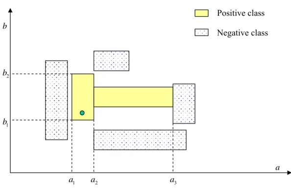
Figure 3.2: Illustration of the concept size of neighbourhood... 57
Figure 3.3: A pseudo-code description of the condition forming procedure... 58
Figure 3.4: The conjunction selection between two continuous attribute-values... 59
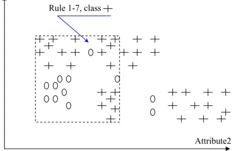
Figure 3.5: Before Pruning, 8 Rules, consistency = 1.00 ... 69
Figure 3.6: Rule 1 merged with Rule 3, consistency = 0.95 ... 69
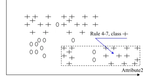
Figure 3.7: Rule 3 merged with Rule 4, consistency = 0.903 ... 70
Figure 3.8: Rule 1 merged with Rule 4, consistency = 0.76 ... 75
Figure 3.9: Rule 1 merged with Rule 7, consistency = 0.67 ... 75
Figure 3.10: Rule 4 merged with Rule 3, consistency = 0.903 ... 76
Figure 3.12: Rule 7 merged with Rule 4-3, consistency = 0.903 ... 78
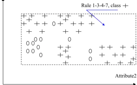
Figure 3.13: Rule 3-1 merged with Rule 4-7, consistency = 0.76... 78
Figure 3.14: Best-RSet, 6 Rules ... 79
Figure 3.15: Final-RSet, with speciafied NL = 10% (Th = 0.9)... 80
Figure 4.1 Graphical representation of the S measure... 98
Figure 4.2 Graphical representation of the TV measure ... 99
Figure 4.3: Classification of an example covered by Rule 1 and Rule 2 ... 102
Figure 4.4: Intersection area of Rule 1 and Rule 2... 103
Figure 5.1 Fuzzy rule generation procedure... 111
Figure 5.2: Output fuzzification ... 115
Figure 5.3: Example set... 117
Figure 5.4: Representation of the example set ... 118
Figure 5.5: Fuzzification of y with Nf = 4... 118
Figure 5.6: Discretised example sets ... 121
Figure 5.7: Rule set obtained for Nf = 4 ... 122
Figure 5.8: Predicted obtained for Nf = 4 ... 122
Figure 5.9: Fuzzification of Y with Nf = 6... 123
Figure 5.10: Rule set obtained for Nf= 6... 123
Figure 5.11: Prediction obtained for Nf = 6 ... 124
Figure 5.3: Output prediction procedure using fuzzy rule... 125
Figure 5.12: The membership degree of attribute 1 = 0.77 ... 126
Figure 5.13: The membership degree of attribute 2 = 0.17 ... 126
Figure 5.14: Example set... 128
Figure 5.15: Fuzzufication of Ay with Nf= 4 ... 129
Figure 5.17: Rule set obtained for Nf=4 using TVFuzz algorithm... 130
Figure 5.18: Prediction of output Ay using DynaFuzz and TVFuzz algorithm ... 131
Figure 5.19: Fuzzufication of Ay with Nf = 10 ... 131
Figure 5.20: Rule set obtained for Nf=10 using DynaFuzz algorithm ... 132
Figure 5.21: Rule set obtained for Nf=10 using TVFuzz algorithm... 133
Figure 5.22: Prediction of output Ay using DynaFuzz and TVFuzz algorithm ... 134
Figure 5.23: Co-ordinate definition of the PUMA 560 robot arm ... 135
Figure 5.24: Prediction of output X using DynaFuzz... 137
Figure 5.25: Prediction of output X using TVFuzz... 137
Figure 5.26: Prediction of output Y using DynaFuzz... 138
Figure 5.27: Prediction of output Y using TVFuzz... 138
Figure 5.28: Prediction of output Z using DynaFuzz ... 139
List of tables
Table 2.1 Training set for the Alarm problem... 26
Table 2.2: Decision table... 43
Table 3.2: Data set... 61
Table 3.2 Test results with comparison between Rules 3 plus, Dyna and RULES-8 ... 84
Table 3.3 Comparison between RULES-8 without pruning and RULES-8 with BPP... 85
Table 3.4 Comparison between BPP and IPP ... 86
Table 3.5 Comparison between Dyna with BPP and RULES-8 with BPP ... 87
Table 4.1: Performance of the H measure, the S measure and the TTV measure when used in Rules-8... 100
Notations
AI Artificial Intelligence Ai The ith attribute in an example.
ML Machine Learning DM Data Mining BPP Basic Post Pruning
CE The class value in example E
CE The Closest Example to SE not belonging to the target class
i R
Cond The condition in rule R for the ith attribute
k j
Cond The kth condition in the ith disjunction
out k
K The kth fuzzy set created for the fuzzification of the output values, Tr(a(k), b(k), c(k))
i k
F The fuzzy set employed in the fuzzy rule R to form a condition on the ith attribute
out R
F The output fuzzy set of the rule R IPP Incremental Post Pruning
IREP Incremental Reduced Error Pruning
n The number of negative examples covered by the newly formed conjunction; N The total number of negative examples (examples not belonging to the target class); Nf The number of output fuzzy sets fixed by the user
N_unclassified The number of examples belonging to the target class and not classified by
the rule set formed so far.
p The number of positive examples covered by the newly formed conjunction; P The total number of positive examples (examples belonging to the target class); P_unclassified The number of examples belonging to the target class and not classified by
the rule set formed so far. S A set of instances. SE A Seed Example
T A training set of examples Th The noise threshold
T_PRSET The Temporary Partial Rule Set Tr Triangular membership function
i E
V The value of the ith attribute in example E
i R
V The discrete value employed in the rule R to form a condition on the ith discrete attribute
max
i
V The maximum known value of the ith continuous attribute
min
i
V The minimum known value of the ith continuous attribute
out E
V The value of the continuous output in example E
max
out
V The maximum known value of the continuous output
min
out
Chapter 1
INTRODUCTION
1.1 Background
In recent years, robust advancements in the field of information technology have made the capacity of data collection and storage increase with incredible speed. Besides, the informationalisation, which is taking place rapidly on a large scale of different socioeconomic activities, has created an immense amount of information. Millions of different databases are being used that hold gigabytes or even terabytes of data. There is a need to tame those enormous sources of data into useful information and knowledge. Data mining, which is now no longer a new concept, has attracted a great deal of attention in the information industry and in society as a whole.
Because of the diversity of disciplines that contributes to data mining, data mining research is expected to generate a large variety of data mining systems. These systems can be categorised as database-oriented, statistics, machine learning, visualisation pattern recognition, neural networks, and so on (Jiawei and Micheline, 2000)
Machine learning is a branch of automatically learn to recognise complex patterns and make intelligent decisions based on the available data. In real applications, inductive learning as an example of such approaches has been one of the most commonly adopted methods for classification besides concept learning and classification learning.
Perhaps the most well known inductive learning method is decision tree induction - a
several input variables. A tree can be learned by splitting the source set into subsets based on an attribute value test. Because of the popularity of this representation technique, many decision tree algorithms have been developed. ID3 (Quinlan, 1986) is one of the most popular algorithms and has been improved several times by a number of researchers ever since it was invented. The most recent versions of this algorithm are C4.5 (Quinlan, 1993) and C5 (Rulequest Research, 2001). Both are integrated into a commercially available software package. Although the decision tree method has a high predictive accuracy and can be easily interpreted by users in using the decision tree for a model, the output attribute must be categorical. The problem is there can be a lot of attributes as the size of data increases, the trees created from numeric datasets can be complex and less efficient.
Another method is rule induction which represents classification knowledge in the form of a
set of rules to describe each class. Like decision tree learning, there are many rule induction algorithms. Among them are AQ (Michalski, 1969; Michalski et al., 1986; Cervone et al., 2001; Michalski and Kaufman, 2001), CN2 (Clark and Niblett, 1989; Clark and Boswell, 1991) and RIPPER (Cohen, 1995). All these algorithms employ the same general method that was used for the first time in the AQ algorithm. AQ21 is the most recent version of the AQ family (Michalski and Wojtusiak, 2006).
The AQ family and some of the algorithms mentioned above have been improved from time to time and have been able to solve some drawbacks of the decision tree. However, since they extract rules and then remove the covered examples from a training set of examples, fragmentation had been one of the problems of these algorithms.
RULES (RULE Extraction System) is a family of simple inductive learning algorithm inspired by ideas from both AQ and CN2. The RULES family is different from the other algorithms in that it does not induce rules on a class-per-class basis but instead considers
the class of the selected seed example as the target class (Shehzad, 2009). It then attempts to induce rules that cover as many examples of the target class as possible using the rule evaluation function. At present, the RULES family has extended to Rules-7 (Pham and Khurram, 2010). Among members of the RULES family, Rules-5 (Pham and Samuel, 2004) is a noteworthy simple but efficient algorithm. It is also known as the Dyna algorithm. Its strength lies in its ability to handle continuous attributes. RULES-5 also employs a more efficient search mechanism as well as a new post-pruning technique (Pham and Bigot, 2004) in order to handle noisy data. Thanks to these advantages, RULES-5 has been successfully employed in different applications. However, it also has drawbacks that prevent it from being adopted for many real-life applications. Hence, there is the need for a new method that is able to achieve good accuracy, compact rule sets and natural induction.
1.2 Aim and objectives
The overarching aim of this thesis is to propose a novel rule induction algorithm, a simple and efficient method which is able to deal with either discrete or continuous variables without the need to preprocess data.
This research is based on RULES-5 (Pham and Bigot, 2004) developed at Cardiff University. This algorithm employs rule forming as a specific method for condition selection based on the consideration of distributions of examples. However, each seed example leads to the creation of a particular rule, and different sequences of seed examples can yield different rule sets. A new method will be developed to make sure that the sequence of seed examples leads to the best rule set. In addition, the new method also improves, the accuracy and simplification of rule forming, as well as expands its real life applications.
Finally, the resulting inductive learning algorithm will be further modified for handling continuous outputs.
To achieve the overall aim of the research, the following objectives were set: - To survey current inductive learning techniques.
- To develop a new simple algorithm that has guidelines for the selection of seed examples. - To design a new heuristic for controlling the rule formation and selection processes. - To develop a new algorithm to handle continuous output using fuzzy logic.
1.3 Methodology
To provide background for this research, an in-depth review of the existing literature was carried out regarding inductive learning techniques and fuzzy logic for inductive learning. The review was intended to cover both discrete and continuous outputs.
It can be said that the inductive learning algorithms devised so far for extracting rules applied for discrete output have helped solve many real life problems. However, in today’s world, the fact that data is accumulating in surmounting volume as well as diversity is exceeding the capability of the existing algorithms. It is necessary, therefore, to invent new algorithms or improve current ones for more effective and beneficial data mining. With respect to this demand in the field, this research presents a new algorithm, RULES-8, and compares it against its predecessor RULES-5 on a diverse population of datasets.
RULES-8 proves to be able to provide a decent result for discrete output, especially when it employs a new heuristic measure to evaluate rule quality. Based on RULES-8, another algorithm – TVFuzz – was designed to deal with continuous output. The new TVFuzz technique was also compared against the DynaFuzz using some real models.
1.4 Outline of the thesis
Chapter 1 provides a brief introduction to the research and states its objectives.
Chapter 2 reviews and gives background information about the research area, including the main inductive learning concepts and descriptions of number of existing algorithms based on these concepts.
Chapter 3 presents a novel rule induction algorithm called RULES-8 that utilises guidelines for the selection of seed examples and proposed a simple method to form rules. This chapter also details an improved pruning method for handling noisy examples.
Chapter 4 designs a new heuristic for controlling the rule formation and selection processes. The performance of the heuristic is compared with that of other heuristics.
Chapter 5 describes a new efficient learning algorithm for continuous output using fuzzy logic theory. This algorithm allows automatic creation of membership functions and produces accurate as well as compact fuzzy sets. It also resolves some drawbacks in RULES-5
Chapter 2
LITERATURE REVIEW
2.1 Preliminaries
Human history has entered its third millennium. The information accumulated over thousands of years has exceeded the capacity of human brains. A perpetuating concern in the science world has been how to make that huge mountain of data useful. Research in this regard has achieved some degree of success, yet scientists are far from being satisfied with what they can learn from the data. During the middle of the 1980s, the concept of Knowledge Discovery from Data (KDD) was conceived and began to help people explore potential knowledge and benefits of immense databases. KDD is a process including several phases among which data mining is the most essential (Jiawei and Micheline, 2000). This is the phase when new information is discovered. The process of knowledge discovery is itself the course of receiving, analysing, applying, and improving the achievements of previous discoveries. Various examples of this area of the science world are database technology, statistics, pattern recognition, information retrieval, neural networks, knowledge-based systems, artificial intelligence, high-performance computing, data visualisation, and so on.
Like other knowledge discovery tools, machine learning (ML) also has the central purpose of “learning from data.” ML algorithms play an essential role in data mining. Most research in machine learning has focused on concept learning or classification learning. The mechanism of this kind of learning is the induction of the definition for a general category from specific positive and negative examples of that category. In real-world
application domains, inductive learning from examples is perhaps the most commonly adopted machine learning approache developed for classification.
Inductive learning is simply known as a process of acquiring knowledge by drawing inductive inferences from data. The study of inductive learning is mainly motivated by the desire to automate the process of knowledge acquisition during the construction of expert systems. This chapter presents a background on machine learning with a focus on inductive learning developed for prediction and classification models. The chapter is organised as follows: Section 2.2 presents a framework for knowledge discovery including input and output format as well as discovery method. Section 2.3 describes in detail inductive learning approaches to classification including major decision tree and rule induction algorithms. Section 2.4 presents some basic concepts of fuzzy logic and existing algorithms for automatic fuzzy rule generation from numerical examples. A summary of the chapter is presented in section 2.5
2.2 A framework for knowledge discovery
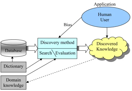
Figure 2.1: A framework for knowledge discovery in databases
Discovery method Search Evaluation Database Discovered Knowledge Human User Application Bias Dictionary Domain knowledge
Figure 2.1 illustrates the basic components of a prototypical system for knowledge discovery in database. In this model, the input includes raw data from the database, information from the data dictionary, additional domain knowledge, and a set of user defined biases that provides a high-level focus. All these will be computed and evaluated by the discovery method so that new knowledge is discovered. Discovered knowledge is the output and can be directed to the user or back into the system as new domain knowledge.
As can be seen in Figure 2.1, the discovery method is the central process designed to extract knowledge from data. This activity usually involves two processes, namely identifying and describing noteworthy patterns in a concise and meaningful manner. The identification process, also referred to as unsupervised learning in ML, categorises or clusters records into subclasses that reflect patterns inherent in the data. The descriptive process, in turn, summarises relevant qualities of the identified classes. This process is known as supervised learning in ML.
Pattern Identification: Discovering pattern classes is a problem of pattern identification or clustering. There are two basic approaches to this problem: traditional numeric methods and conceptual clustering. Traditional methods of clustering come from cluster analysis and mathematical taxonomy (Dunn and Everitt 1982). These algorithms produce classes that have a maximum level of similarity within classes but a minimum level of similarity between classes. Various measures of similarity have been proposed, most based on Euclidean measures of distance between numeric attributes. Accordingly, these algorithms only work well on numeric data. An additional drawback is their inability to use background information, such as knowledge about similar cluster shapes. There have been attempts in conceptual clustering to overcome these problems. These methods work with
nominal and structured data and determine clusters not only by attribute similarity but also by conceptual cohesiveness, as defined by background information.
Although successful under certain conditions, these methods do not always equal the human ability to identify useful clusters, especially when dimensionality is low and visualisation is possible. This situation has prompted the development of interactive clustering algorithms that combine the computer’s computational powers with the human user’s knowledge and visual skills.
Concept Description: Describing the useful pattern classes once having been identified is a more important task than just simply enumerating them. In machine learning, this process is known as supervised concept learning from examples, i.e. to derive an intentional description of a class given a set of objects labeled by class. Empirical learning algorithms, the most common approach to this problem, work by identifying commonalities or differences among class members. Well-known examples of this approach include decision tree inducers (Quinlan 1986), rule induction (Michalski et al 1969), neural networks (Rummelhart and McClelland 1986), and genetic algorithms (Holland et al. 1986).
Some learning approaches, such as explanation-based learning (Mitchell, Keller, and Kedar-Cabelli 1986), require a set of domain knowledge (called a domain theory) in order to explain why an object falls into a particular class. Other approaches combine empirical methods and knowledge-based ones. The main drawback of empirical methods is their inability to use available domain knowledge. This failure can result in descriptions that encode obvious or trivial relationships among class members. Discovery in large, complex databases clearly requires both empirical methods to detect the statistical regularity of patterns and knowledge-based approaches to incorporate available domain knowledge.
Because different tasks require different forms and amount of information, they often influence discovery algorithm selection or design. The next section discusses a learning method developed for classification model.
2.3 Inductive learning for classification model
The concept of learning has been tackled by many authors. Simon (1983), on a broader term, defined learning as changes in the system that are adaptive in the sense that they enable the system to do the same task or tasks drawn from the same population more efficiently and more effectively the next time. Shavlik and Dietterich (1990) narrowed it down to describe inductive learning, which is a process accomplished by reasoning from supplied examples to produce general rules.
Inductive learning can be categorised as either supervised inductive learning or unsupervised inductive learning (Afify, 2004). In supervised learning a supervisor gives direct feedback to the learner about the appropriateness of its performance. This is in sharp contrast to unsupervised learning where this kind of feedback is absent. Since this thesis focused on supervised inductive learning procedures, all the algorithms discussed in this section refer to supervised inductive learning methods.
2.3.1 Decision tree learning
The major purpose of the decision tree method is to select step by step an attribute to decompose training set into several subsets until there remains a unique class in each subset. The result of this method generally takes the form of a tree, with class names as leaves and other nodes representing attribute-based tests for possible outcomes as branches.
Let S represent an example set and
{
1, 2,... n}
A= A A A be the condition attribute set with observable value sets i
{
1i, ,...,2i i}
n
V = V V V respectively. C is the decision attribute with domainC=
{
C C1, 2,...Ck}
. The general decision tree inductive learning procedure is as follows:Step1: Select attribute th
i to decompose example set S into S Si1, i2,...,Sin (n is possible value
of attribute th
i ). For a continuous attributeAi, a binary test is carried out, and a corresponding branch i i
t
V <V is created, with a second branch corresponding to i i t
V >V , where i
t
V is a threshold in the domain ofAi)
Step 2: For each subsetSik, if there is a unique class in it, then stop decomposing, and label
the node as a class. Otherwise, continue to decompose Sik in the same way as described in step 1.
Table 2.1 shows an example data set and Figure 2.2 displays a decision tree constructed from this data.
Table 2.1 Training set for the Alarm problem
Example Sensor_1 Sensor_2 Alarm
1 -1 0 OFF 2 0 0 OFF 3 -1 1 ON 4 0 1 OFF 5 0 1 OFF 6 1 1 ON 7 -1 0 OFF 8 -1 1 ON
Figure 2.3: Representation of the formed decision tree
-1 0 OFF 1 OFF 0 1 ON ON Sensor_1 Sensor_2
In order to classify an object, one starts at the root of the tree, evaluate the test, and takes the branch appropriate to the outcome. The process continues until a leaf is encountered, at which time the object is asserted to belong to the class named by the leaf.
The earliest Decision tree learning system is Concept Learning System (CLS). It was introduced by Hunt et al (1966). In the CLS series, Hunt decomposes S by using a heuristic look-ahead method which utilises values which appear most frequently. CLS has nine versions, numbered from CLS1 to CLS9. The main difference between the first eight versions and the latest version CLS9 is that the former versions use only binary decomposition while CLS9 can provide non-binary decomposition.
In 1983, Quinlan presented the ID3 inductive learning algorithm [Quinlan 1983], also a descendant of the CLS. ID3 uses an information entropy measure to guide the decomposition.
Information entropy is defined as:
2 ( ) ( i, ) log ( i, ) i I S = −
∑
p C=C S p C=C S (2.1) i ik ik i j i j A v v V |S | E(A ,S) I(S ) |S| = ∈ =∑
(2.2)Where (p C=C Si, )be the proportion of instance in S
I(S) is the whole information entropy in set S
E(Ai,S) denotes the information entropy when S is divided based on the condition attribute Ai.
The information gain is defined as:
( , )Gain A Si =I S( )−E A S( , )i . (2.3)
ID3 chooses the optimal decomposition at a node by maximising the information gain (Pitas et al. 1992).
By using the information gain as a guide, ID3 tends to choose the decomposition based on the condition attribute that has more values. This might cause ID3 to miss more general decision trees. Therefore, Quinlan introduced the information gain ratio to overcome this weakness (Quinlan 1986a). The information gain ratio is defined as:
( ) ( , ) _ ( , ) ( ) i i i I S E A S Gain ratio A S IV C − = (2.4)
Where ( )IV Ai denotes the degree of randomness of the distribution of the examples in S
when partitioned using Ai
i ik ik i j j i 2 A v v V |S | |S | IV(A ) log ( ) |S| |S| = ∈ = −
∑
(2.5)ID3-IV is a version of the ID3 family, modified with the information gain ratio (Quinlan 1986a) and named by Cheng (Cheng et al. 1988). Cheng et al. (1988) continued to introduce Generalised ID3, or GID3. GID3 uses the information gain ratio and only generates a new branch (i.e. forms a new subset) when encountering a relevant value. The relevance of a value is evaluated by a user-determined tolerance level. This modification is intended to avoid over-specific decision trees.
PRISM is based on ID3 but uses a modified information entropy measure which tries to reduce redundant condition values in the learning output (Cendrowska 1988).
Subsequent to ID3 were ID4 (Schlimmer and Fisher 1986), ID5 (Utgoff 1988), ID5R and ID5R-hat (Utgoff 1989).
C4.5 is an industrial version of ID3 (Quinlan 1993). It has the same basic structure as ID3-IV. It features pruning of decision trees and then conversion of the pruned decision trees into rule sets. In addition, C4.5 can handle continuous values, noise and missing values. Breiman et al. (1984) present CART (Classification and Regression Trees). CART is designed for handling continuous-valued examples. In such examples, all the condition attributes have continuous values and the decision attribute has discrete values. As a Decision tree inductive learning method, CART can only generate binary decision trees. It uses the Gini index of diversity denoted by i(t). As a measure of node impurity to guide the decomposition of the example set at a node t, i(t) is defined as follows:
( ) ( | ) ( | )
j k
i t p j S p k S
≠
=
∑
(2.6)Where S denotes the set at node t, j and k are classes in set S and p(j|S), p(k|S) denotes the probability of examples of class j and k in set S in turn.
Let S represents a continuous-valued example set and
{
1, 2,... n}
A= A A A be the condition attribute set. The learning process of CART can be briefly described as follows:
At a node t, CART searches through the condition attributes
{
1, 2,... n}
A A A one by one. For each condition attribute, it finds the best decomposition by maximising the decrease of impurity. Then, it selects the best decomposition from n candidates.
Clearly, at a node, the best decomposition is dependent on the measure of impurity. When that measure changes, the best decomposition will also change.
Crawford presents an extension of CART (Crawford 1990), OC1, which is able to generate oblique decompositions (Murthy et al. 1994). The oblique decomposition is the decomposition that is not parallel to coordinate axes in example sets. A smaller decision tree can be generated by using oblique decomposition.
2.3.2 Rule induction
Mitchell (1978) introduced the Candidate-Elimination algorithm, which served as the basis to develop the Rule induction method. The Rule induction method is to establish a hypothesis rule space which is based on a given example set and then to refine (search through) the hypothesis rule space to find more general rules. The hypothesis rule space is also called the version space.
Among the rule inductive methods devised based on the Candidate-Elimination algorithm is Cohen and Feigenbaum’s (1982) Extension-Against method. The algorithm is described as follows.
Let S be an example set. The examples are categorised as either positive or negative according to their classes. If an example belongs to the class of interest, it is considered positive. Examples belonging to all other classes are considered negative.
H denotes the version space. Initially, H contains all the possible concepts which are based on the given positive examples. Then, as examples are presented, candidate concepts are eliminated from H. The elimination process goes on until only one kind of concept for the same class remains in H, and this is the desired kind of concept. The procedure can be described in more details as follows:
When a positive example is presented, H will be generalised, that is, specific concept descriptions are removed from H. When a negative example is presented, H will be specialised, that is, very general concept descriptions are removed from H. In this way, H gradually shrinks until only the desired concept descriptions remain. The learned concept is represented in the form “IF [description] THEN [decision]”.
This algorithm can find the most acceptable concepts based on the given example set. However, for a large example set, it can be very difficult or even impossible to construct the initial H.
Perhaps one of the best known Rule induction methods is AQ algorithm. Credited to Michalski (1975), this algorithm is similar in principle to the Candidate-Elimination algorithm. The main difference is that, initially, H contains the null description (the most general concept) only. Let an example set S be divided into a positive set S+and a negative setS−. The examples in S+ are in the same class, and S+∪S−=S and S+∩S−=∅. The basic idea in the AQ algorithm is to find a cover CV(S+|S−) which covers S+ against S−,
that is, it separates S+ from S−. A simplified version of the AQ algorithm is as Figure 2.3 follows:
Step1: Randomly select a “SEED” example e from the positive examples setS+.
Step 2: Generate an orderly disjoint "START" G(e|S−), e∈S+. The star is against the setS−. Step 3: Find the “best rule” from the START according to user-defined criteria. Remove the examples covered by this rule from S+.
Step 4: If the positive example set S+ is not empty, return to step 1 and continue the procedure. Otherwise, the obtained rules constitute a complete and consistent concept of
S+.
In the most general sense, the START G(e|S−) of example e, e∈S+, is a set of all possible alternative non-redundant descriptions of example e that do not cover examples in S−. S−thus acts as a constraint on the possible descriptions of e. The START can be generated using a number of methods (Michalski 1983) which constitute the kernel of the AQ algorithm.
The advantages of AQ are two-folds: first, because the search is based on a Seed Example (SE), AQ will find the shortest descriptions for a concept; second, AQ can control the concepts forming procedure by using some user-defined criteria.
Various AQ based inductive learning algorithms have been developed such as AQ11 (Michalski 1983) and AQ14-NT (Pachowicz and Bala 1991). AQ15 is an incremental version of AQ11 (Michalski et al. 1986). AQ15-GA incorporates a genetic algorithm technique to guide the search (Vafaie and DeJong 1994). Some multistage versions of AQ based algorithms, AQ17-DCI, AQ17-FCLS, AQ17-HCI and AQ17, have also been reported (Wnek and Michalski 1994). Over the past decades, AQ algorithms have continued to be developed into a series of learning algorithms called the AQ family. The most recent member of the AQ family is AQ21 (Wojtusiak and Michalski, 2006).
Another renowned method is CN2 (Clark and Niblett, 1989). It is a rule induction algorithm named after its authors. CN2 attempts to combine the good features of the decision tree algorithm ID3 with the rule induction algorithm AQ. CN2 uses a subset of the expression language VL1 used in AQ and also retains the beam search strategy of AQ. However, it differs from AQ in that it does not rely on specific examples during search but instead considers all specialisations of a complex similar to ID3, which considers all attributes in order to find the best one to split at a particular node. The specialisation of a complex involves either adding a new conjunctive term or removing a disjunctive element
in one of its selectors. Because of this top-down search for complexes, the CN2 algorithm is able to incorporate a cutoff method similar to the one used in decision tree pruning that can halt specialisation of a complex when no further statistically significant specialisations can be found. This results in an extension of the search space to include rules that do not perform perfectly on the training data.
Similarly to ID3, to handle continuous attributes CN2 algorithm divides the range of values of each attribute into discrete subranges and then creates two thresholds on the attribute at subrange boundaries. One advantage is that CN2 also includes any missing values for both discrete and continuous-valued attributes. In case of discrete attributes, the missing value is replaced with the most commonly occurring value of that attribute in the training data. For continuous attributes, the mid-value of the most commonly occurring subrange is used to replace any missing values.
The original version of CN2 produces an ordered set of rules. In the case where an example satisfies none of the rules, it is classified using the default rule at the end of the list, which assigns it the class label of the most frequently occurring class within the training data. CN2 uses two rule evaluation measures, namely entropy and statistical significance. The latter is measured using the likelihood ratio statistic (Kalbfleish, 1979) which is defined as:
1 ( , ) 2 log n i i i i f LikelihoodRatio F E f e = =
∑
(2.7)The function assesses the significance of the complex by comparing the observed frequency fi of examples satisfying the complex among classes with the expected
frequency ei if the rule made random predictions.
The CN2 algorithm has been modified in a later version (Clark and Boswell, 1991), which enables it to generate an unordered set of rules. It also replaced the entropy rule evaluation measure with the Laplace expected error estimate which is given by:
cov cov 1 ( , , ) class class ered ered n LaplaceAccuracy n n k n k + = + (2.8) Where class
n is the number of examples of the target class covered by the rule
covered
n is the total number of examples covered by the rule
kis the number of classes
The modified algorithm also incorporates a stopping criterion to check if the Laplace estimate of the best complex is better than that of the default rule. If this is the case, the induction continues for the current class. Otherwise, the new complex is not deemed to bring about an improvement and so rule generation for the current class terminates. Since the new version of CN2 generates an unordered set of rules, so a conflict resolution approach is also adopted in order to resolve any clashes that might occur. In case a new example satisfies more than one rule predicting different classes, a probabilistic method is
used in which the distribution of covered examples of each rule among classes is summed to find the most probable class.
Among the more recent methods of rule induction is the RULES family. RULES (RULe Extraction System) is a family of simple inductive learning algorithms which inherit ideas from both AQ and CN2 algorithms. The RULES family is different from the other algorithms in that it does not induce rules on a class-per-class basis but considers the class of the selected seed example as the target class. It then attempts to induce a rule that covers as many examples of the target class as possible using the rule evaluation function. In addition, the RULES family only marks the examples covered by previous rules instead of removing them.
RULES (Pham and Aksoy, 1993), RULES-2 (Pham and Aksoy, 1995b) and RULES-3 (Pham and Aksoy, 1995a) were the first three algorithms in the family. Later, Pham and Dimov developed a new rule induction algorithm RULES-3 Plus (Pham and Dimov, 1997b) that incorporated the beam search strategy instead of greedy search and used a new rule evaluation measure called the H-measure (Lee, 1994), which is defined as:
[2 2 . 2 (1 )(1 )] p n p P p P H P N p n P N p n P N + = − − − − + + + + + (2.9)
Where, P is the total number of positive examples (examples belonging to the target class); N is the total number of negative examples (examples not belonging to the target class); p is the number of positive examples covered by the newly formed rule;
At present, the RULES family has extended to Rules-7 (Shehzad, 2010). Among members of the RULES family, Rules-5 (Bigot, 2004) is a noteworthy simple but efficient algorithm.
2.3.3 Rules-5 algorithm
Rules-5 (Bigot, 2004) is also known as the Dyna algorithm, which is described in Figures 2.5 and 2.6. In the Dyna algorithm, the search strategy employed is based on seed examples. Each seed example leads to the creation of particular rules, and different sequences of seed examples can yield different rule sets. Thus, a guideline for selection of the seed examples needs to be developed in the later version.
It should be noticed that in the Dyna algorithm, a new heuristic for rules evaluation is designed. The heuristic is defined as follows:
1 new unclassified p p n S p n P N − − ⎛ ⎞ = ⎜ − ⎟ + ⎝ ⎠ (2.10)
Where: P is the total number of positive examples (examples belonging to the target class); N is the total number of negative examples (examples not belonging to the target class);
p is the number of positive examples covered by the newly formed rule;
n is the number of the negative examples covered by the newly formed rule.
p_new is defined as the number of positive examples covered by the newly formed conjunction of conditions and not covered by previously created rules
P_unclassified is defined as the number of examples belonging to the target class and not classified by the rule set formed so far
Step 1: Select Seed example (SE), SE is considered a positive example
Step 2: Find conditions of a new rule according to a consideration of distribution of examples by looking for the closest example (CE) not belonging to the target class and covered by the rules formed so far
Step 3: If there are uncovered examples, go back to Step 1
Figure 2.5 Dyna rule forming procedure
Figure 2.6: Graphical representation of the coverage of the new rules
Most inductive learning algorithms dealing with discrete classes use a similar input data structure. The following section discusses another trend of learning for handling continuous classes.
Attribute1
Attribute2 SE
2.4 Learning fuzzy logic from examples
Fuzzy set theory has been in existence for almost half a century and has been proved extremely useful in many control applications as well as non-control applications requiring decision-making in uncertain environments. This section summarises some basic concepts of fuzzy logic and existing algorithms for fuzzy inductive algorithms.
2.4.1 Fuzzy logic basic concepts
- A fuzzy set F defined on U is characterised by its membership functionμF( ) [0,1]u ∈ (Klir and Folger, 1992),μF( )u is the degree of membership. μF( ) 0u = means that u does not belong to the fuzzy set and μF( ) ]0,1]u ∈ means that u belongs to the fuzzy set with a degree of certainty ofμF( )u .
- Membership function ( )μF u maps the degree to which an element u belongs to a fuzzy subset F from domain U to the range [0,1]
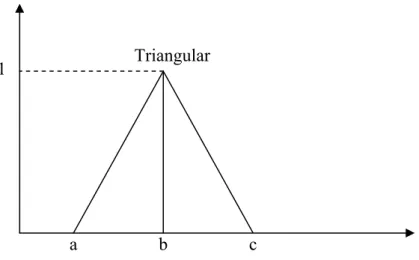
Supposing that U is the set of all non-negative integers and F is a fuzzy subset of U labeled "approximately 10," then, the fuzzy subset can be represented by a membership function,μ10( )u . Figure 2.7 depicts a possible definition of the membership function.According to this fuzzy subset, the number 10 has a membership value of 1.0 (i.e., 10 is exactly l0), and the number 9, a membership value of 0.5 (i.e., 9 is roughly 10 to the degree of 0.5). Note that a membership function in general can be linear, trapezoidal, convex curve, or in many other forms (Lee 1990, Dummerrnuth 1991) but to facilitate computation, triangular forms are widely adopted because they are easy to define as Tr(a,b,c) (Figure 2.8) This representation will be employed in this study.
Figure 2.7: MF defining the concept "approximately 10" on a fuzzy system.
Figure 2.8: Triangular membership functions
Approximately 10 U: Set of nonnegative integers 1 8 10 12 Triangular 1 a b c
- A fuzzy rule R is composed of a number of possible fuzzy conditions on each of the m attributes and an output fuzzy set ( out)
R
F it can be represented as follows:
1 ... i ... m out
R R R R
Cond ∧ ∧Cond ∧ ∧Cond →F
2.4.2 Fuzzy logic system
Fuzzy Logic Systems (FLS) are one of the main developments and successes of fuzzy logic. They are motivated by the biological brain’s ability to learn, reason and generalise using noisy or uncertain information (Lei 1999).
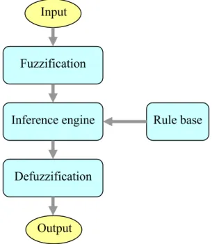
A general structure of a fuzzy logic system consists of four units including fuzzification, defuzzification, inference engine, and rule base (Dadone 2001; Lee 1990a; Passino and Yurkovich 1998). A general structure of a fuzzy logic system is described in Figure 2.9
Figure 2.9: A general structure of a fuzzy logic system
To illustrate these steps, the following example (Grabot, 1998) will be used. A fuzzy rule set is needed in order to control a car moving towards a wall, bringing it close to the wall
Fuzzification Inference engine Defuzzification Rule base Output Input
in the most efficient way. There are two attributes, the speed of the car (Speed∈
[
0km h/ ,60km h/]
), and its distance from the wall (Distance∈[
0 ,60m m]
), and one output, the deceleration ( 0 / ,12 /2 2Brake∈ ⎣⎡ m s m s ⎤⎦).
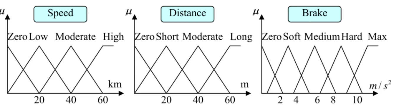
a. Fuzzification
Fuzzification is the process which translates measured values into real values between 0 and 1. It also assigns these values degrees of truth, usually called membership degrees, for the linguistic values of the input linguistic variables. For the instance above, the tree parameters are decomposed as follows (Figure 2.10):
The linguistic variables of attribute Speed is divided into the following fuzzy sets: zero, low, moderate and high.
The linguistic variables of attribute Distance is divided into the following fuzzy sets: zero, short, moderate and long.
The linguistic variables of attribute Brake is divided into the following fuzzy sets: zero, soft, medium, hard and max.
Figure 2.10: Decompose in membership function
2
ZeroSoft Medium Max
μμ Brake Hard 4 6 8 10 2 / m s 20 40 60
ZeroShort Moderate Long μ
μ Distance
m 20 40 60
Zero Low Moderate High μ
μ Speed
b. Rule base
The rule base of a fuzzy logic system consists of a set of fuzzy IF-THEN rules. To help the generation of all rules, the typical method of multidimensional matrix representation called the decision table. Each cell in the matrix is called a fuzzy subspace and represents a possible rule when linked with a particular output. Table 2.2 shows the decision table generated from the previous example.
Table 2.2: Decision table
Speed Distance Zero Short Moderate Long
Zero Zero Zero Zero Zero
Low Max Medium Soft Zero
Moderate Max Hard Medium Zero
High Max Hard Medium Zero
Rule base set includes:
1. IF [Speed = Zero] and [Distance = Zero] THEN [Brake = Zero] 2. IF [Speed = Zero] and [Distance = Short] THEN [Brake = Zero] 3. IF [Speed = Zero] and [Distance = Moderate] THEN [Brake = Zero] 4. IF [Speed = Zero] and [Distance = Long] THEN [Brake = Zero] 5. IF [Speed = Low] and [Distance = Zero] THEN [Brake = Max] 6. IF [Speed = Low] and [Distance = Short] THEN [Brake = Medium] ….
c. Reference engine
Since fuzzy logic systems are stimulated by the biological brain’s capability to make decisions, the inference engine or fuzzy reasoning is considered a method of cloning a human decision making process of judging and giving a proper fuzzy output depending on the inputs and the rule base
d. Defuzzification
Defuzzification is the mapping from the linguistic fuzzy output defined over an output universe into a crisp output space (Awadalla 2005). There are many defuzzification strategies. The most common strategies are the Weighted Average, Mean of Maxima and Centroid.
- Weighted Average method used the formula:
1 1 _ ( ). _ ( ) r R out R r R R rule E C output rule E μ μ = = =
∑
∑
Where E is the new example,
out
C is the centre of the output fuzzy set of the considered rule r is the total number of rules
- The Mean of Maxima method (MoM): This method selects the mean of output values within the group of possible output fuzzy sets that correspond to the highest membership degree. If more than one solution exists, the mean is taken. A graphical example can be seen in Figure 2.11.
- The Centre of Gravity method (CoG): This method was first suggested by Zadeh (Roychowdhury and Wang, 1996). The output value is obtained by assessing the centre of gravity of the resulting group of fuzzy sets (considering overlapping or not). A graphical example is shown in Figure 2.12. This method can be highly computationally costly since the centre of gravity might not always be easy to assess, in particular when considering overlapping.
Figure 2.11: M.o.M defuzzification
Figure 2.12: C.o.G defuzzification
μμ u Mean value Maximum degree ( )u μ u Gravity centre, if ignoring
the overlapping
( )u μ
u Gravity centre, if considering
2.4.3 Generating fuzzy rule from numerical data
Perhaps the most popular method is the Wang and Mendel algorithm (Wang and Medel, 1991). The method determines a mapping from the input space to the output space based on the combined fuzzy rule base using a defuzzification procedure. Follows is a detailed description of this method:
Step 1: Divide the Input and Output Spaces into Fuzzy Regions
Step 2: Generate Fuzzy Rules from the Given Data Pairs
Step 3: Assign a Degree to Each Rule
Step 4: Create a Combined FAM Bank
Step 5: Determine a Mapping based on the FAM Bank
Figure 2.13: Wang and Medel procedure intended to generate fuzzy rules
The mapping was proven to be capable of approximating any real continuous function to an arbitrary accuracy. However, as mentioned by the authors, there is a problem of “growing memory”: when more training examples become available, more rules are generated and the selection of the best rules becomes difficult. To help this selection, Delgado and Gonzalez use a method based on the definition of frequencies in each fuzzy domain, which allows one to identify if any possible rule is a “true rule”(Delgado and Gonzalez, 1993).
Similar to Wang and Mendel’s algorithm, Nozaki and Ishibuchi (1997) proposed to use a particular heuristic method to automatically generate fuzzy if-then rules from numerical data. The fuzzy if-then rules with non-fuzzy singletons (i.e., real numbers) in the consequent parts are generated by assessing single real numbers (instead of membership functions) which are to be stored in each cell of the decision table. Since there is no defuzzification step involved, Nozaki and Ishibuchi’s algorithm is quite simple. However, the problem of growing memory still remains.
Sebag and Schoenauer(1994) observed that the problem of designing membership functions might be just as complex as designing fuzzy rules. Both methods above need to pre-define membership functions, which is actually not an easy task. Various methods for automatic creation of membership functions have been devised. However, all still cannot solve the existing problems, not to mention the rise of new problems. One of the challenges is the demand of post-processing the large fuzzy rule sets formed to acquire more compact rule sets.
To resolve the problems for automatic membership functions design, Hong and Lee (1996) proposed a method, by which the fuzzification of output is performed using a clustering procedure that regards examples in the training set (T) with close output values as belonging to the same fuzzy set. Appropriate membership functions are then assigned to represent each fuzzy set. Initial membership functions are assigned to attributes in the form of a triangle base equal to a small interval predefined by a user. After attributes have received their initial membership functions, the decision table is built using the examples in T. The decision table is then simplified through the process of merging membership functions from which the final rule sets can be extracted.
Nevertheless, a problem still exists with the merging process regardless of the attempt to improve it by the authors Hong and Lee (1999). That is, it can be highly computationally expensive as the number of attributes increases. Hong and Chen (2000) also attempted to develop a method to simplify the initial membership functions. Their method has been proven to be more efficient and accurate, yet it does not reduce considerably the computational cost. This method, however, generates a set of fuzzy rules where the membership functions have been automatically created and the universes of discourse are not equally partitioned. It should be noted that it is still a challenge when the number of attributes increases.
Another type of algorithms based on machine learning techniques was developed by Shann and Fu (1995). This algorithm uses the neural network structure that allows the use of the error back-propagation learning algorithm for fuzzy rule generation. However, one of the weaknesses of this algorithm is that the membership functions need to be predefined. There are many other algorithms using neural networks and most of them use a method similar to Shann and Fu’s algorithm.
In Yuan and Shaw (1995), continuous attributes are first fuzzified using human experts or techniques such as fuzzy clustering, and then the membership functions are employed by each attribute as possible branches during the construction of the decision tree. However, this algorithm is designed for classification problems only and it is not clear how it would handle real or fuzzy outputs. In addition, the membership functions also need to be predefined.
Perhaps the most common way of creating fuzzy decision trees is to use a method similar to the FILM algorithm (Jeng et al., 1997) where a crisp decision tree is first created using ID3 and then fuzzification operations are applied to modify it. The membership functions
are created automatically, but the models can only be used for problems with discrete outputs; fuzzy logic is only employed to handle vagueness and ambiguity in the attribute values.
Other methods also exist. Wang et al. designed an algorithm based on the PRISM learning strategy (Wang et al., 1999). More recently, a method was proposed using a combination of inductive learning and genetic algorithms (Castro et al., 2001). However, like many others (Ravi et al., 2001; Wang et al., 2001), all these fuzzy inductive learning methods have been developed only for classification problems where the fuzzy concepts are used to deal with noise, uncertainty and imprecision in the attribute values.
In 2004, Bigot released a new technique called DynaFuzz that can automatically create input membership functions. Inheriting the advantages of its predecessors – theDyna and DynaSpace inductive learning algorithms, DynaFuzz can generate more compact and more accurate fuzzy rule sets. However, in the present world, given that databases are becoming more diverse with more features as well as bigger quantity, there is an increasing need for improving existing algorithms and developing new ones. The need for further research on the automation of creating output membership functions is also of no exception.
2.5 Summary
This chapter has given background information on different machine learning algorithms with attention focused on inductive learning. The basic concepts of inductive learning algorithms have been described and the two main types of these algorithms currently available presented. The chapter has also presented the basic concepts of fuzzy logic relevant to fuzzy rule generation. Finally, existing algorithms for automatic rule generation based on these concepts are discussed.
Chapter 3
RULE 8: A NOVEL RULE INDUCTION LEARNING ALGORITHM
3.1 Preliminaries
Ian and Eibe (2005) observed, “We are overwhelmed with data. The amount of data in the world, in our lives, seems to go on and on increasing and there is no end in sight.” Achievements of digital archive technology have especially reinforced this observation. Everyday, a huge amount of data is being accumulated in all social, economic, technological, and production activities and is becoming highly valuable resources which could support or lead people to new understandings in socio-economic networking, in manufacturing as well as in scientific research activities. A challenge for scientists across different disciplines has been how to optimise the process of acquisition of knowledge from data.
Inductive learning is a form of data analysis that can be used to extract models that are able to describe important data classes or predict future data trends. Such analysis can provide a better understanding of the data at large. In machine learning, many inductive methods have been proposed. They can be divided into two main categories, namely decision tree induction and rule induction.
In rule induction, the search strategy employed is based on seed examples. Each seed example leads to the creation of particular rules, and different sequences of seed examples can yield different rule sets. In the current version of these algorithms there is no guideline for the selection of seed examples. The first uncovered example found in the training set (T) is always selected, and therefore the rule set created will depend on the storage order of the examples in T.
This chapter presents RULES-8, a proposed new rule induction algorithm that addresses the weaknesses of the predecessors. In particular, it selects a candidate attribute-value instead of a seed example to form a new rule to make sure that the candidate attribute-value leads to the best rule. The conjunction is also formed by incrementally adding conditions which are selected by utilising a specific heuristic measure. In addition, a rule simplification technique is also improved to create more compact rule sets and minimises overlapping between rules.
The chapter is organised as follows: Section 3.2 gives a detail description of the new rule induction algorithm. Section 3.3 discusses in detail the problems identified with Pruning techniques in Dyna algorithm. An improvement pruning technique will also be presented in this section. The next section, Section 3.4, provides the results obtained from an experimental evaluation of RULES-8 on some benchmark datasets. Finally, section 3.5 summarises and concludes the chapter.
3.2 The Novel Learning Algorithm
3.2.1 Representation and Basis concepts
Like its predecessors, RULES-8 also extracts IF-THEN rules directly from a set of examples called the training set (T). Each example is described by a vector of value pairs, together with a specification of the class that belongs. Uncovered attribute-value pairs are attribute-attribute-values in uncovered examples.
Conditions on nominal attributes are equality tests of the form [Ai =vij], where Ai is the
inequalities of the form [Ai >ti1] or [Ai ≤ti2], where ti1 and ti2 are two thresholds in the domain of attributeAi.
Seed attribute-value is a candidate condition, which if being applied to a rule, the newly-created rule will be capable of covering the most examples
An attribute-value constitutes a condition. If the number of attributes is na, a rule may contain between one or naconditions, each of which must be a different attribute-value. Only the conjunction of conditions is permitted in a rule and therefore the attributes must all be different if the rule comprises more than one condition.
The class to be learned is called the target class. Examples of the target class in the training set are called positive examples. Examples in the training set that do not belong to the target class are called negative examples.
A rule is said to cover an example if the example satisfies all the rule conditions. A rule is said to be consistent if it covers none of the negative examples in the training set, and it is complete if it covers all the positive instances in the training set.
3.2.2 Learning algorithm description
Unlike its predecessors in the RULES family and other rule induction techniques, the new learning algorithm begins by selecting a seed value. Based on the seed attribute-value, this algorithm employs a specialisation process searching a general rule by incrementally adding new conditions to them.
To select the best conjunction of conditions, a heuristic H measure is also used to assess the information content of each newly formed rule. It can be defined as follows:
[2 2 . 2 (1 )(1 )] p n p P p P H P N p n P N p n P N + = − − − − + + + + + (3.1) Where
P is the total number of positive examples (examples belonging to the target class);
N is the total number of negative examples (examples not belonging to the target class);
p is the number of positive examples covered by the newly formed rule;
n is the number of the negative examples covered by the newly formed rule.
The following figure describes the procedures of the newly proposed inductive learning algorithm.