Machine learning algorithms for cognitive radio wireless networks

(1)

Machine Learning Algorithms for Cognitive

Radio Wireless Networks

by

Olusegun Peter Awe

A Doctoral Thesis submitted in partial fulﬁlment of the requirements for the award of the degree of Doctor of Philosophy (PhD)

November 2015

Signal Processing and Networks Research Group,

Wolfson School of Mechanical, Manufacturing and Electrical Engineering, Loughborough University, Loughborough,

Leicestershire, UK, LE11 3TU

c

(2)

CERTIFICATE OF ORIGINALITY

This is to certify that I am responsible for the work submitted in this thesis, that the original work is my own except as speciﬁed in acknowledgements or in footnotes, and that neither the thesis nor the original work contained therein has been submitted to this or any other institution for a degree.

... (Signed)

(3)

I dedicate this thesis to my wife, Oluwakemi Awe, my son, Ifemayowa Awe, my daughter, Ifemayokun Awe and the memory of my late father,

(4)

Abstract

In this thesis new methods are presented for achieving spectrum sensing in cognitive radio wireless networks. In particular, supervised, semi-supervised and unsupervised machine learning based spectrum sensing algorithms are developed and various techniques to improve their performance are described. Spectrum sensing problem in multi-antenna cognitive radio networks is considered and a novel eigenvalue based feature is proposed which has the capability to enhance the performance of support vector machines algorithms for signal classiﬁcation. Furthermore, spectrum sensing under multiple pri-mary users condition is studied and a new re-formulation of the sensing task as a multiple class signal detection problem where each class embeds one or more states is presented. Moreover, the error correcting output codes based multi-class support vector machines algorithms is proposed and investigated for solving the multiple class signal detection problem using two diﬀerent coding strategies.

In addition, the performance of parametric classifiers for spectrum sens-ing under slow fadsens-ing channel is studied. To address the attendant per-formance degradation problem, a Kalman filter based channel estimation technique is proposed for tracking the temporally correlated slow fading channel and updating the decision boundary of the classifiers in real time. Simulation studies are included to assess the performance of the proposed schemes.

Finally, techniques for improving the quality of the learning features and improving the detection accuracy of sensing algorithms are studied and a novel beamforming based pre-processing technique is presented for feature realization in multi-antenna cognitive radio systems. Furthermore, using the beamformer derived features, new algorithms are developed for multiple

(5)

ii

hypothesis testing facilitating joint spatio-temporal spectrum sensing. The key performance metrics of the classiﬁers are evaluated to demonstrate the superiority of the proposed methods in comparison with previously proposed alternatives.

(6)

3.3.1 Naive Bayes Classifier Model Realization 33 3.3.2 Naive Bayes Classifier for Gaussian Model 34 3.4 Nearest Neighbors Classification Technique 35 3.4.1 Nearest Neighbors Classifier Algorithm 36 3.5 Fisher’s Discriminant Analysis Techniques 37 3.6 Support Vector Machines Classification Techniques 40

3.6.1 Algorithm for the Realization of Eigenvalues Based Feature Vectors for SUs Training 41 3.6.2 Binary SVM Classiﬁer and Eigenvalue Based Features

for Spectrum Sensing Under Single PU Scenarios 44 3.6.3 Multi-class SVM Algorithms for Spatio-Temporal

Spec-trum Sensing Under Multiple PUs Scenarios 49 3.6.4 System Model and Assumptions 50

3.6.5 Multi-class SVM Algorithms 55

3.6.6 Predicting PUs’ Status via ECOC Based Classiﬁer’s

Decoding 59

3.7 Numerical Results and Discussion 63

3.7.1 Single PU Scenario 63

3.7.2 Multiple PUs Scenario 68

3.8 Summary 74

4 ENHANCED SEMI SUPERVISED PARAMETRIC

CLAS-SIFIERS FOR SPECTRUM SENSING UNDER FLAT

(8)

Contents iii

4.1 Introduction 75

4.2 K-means Clustering Technique and Application in Spectrum

Sensing 76

4.2.1 Energy Features Realization 78 4.2.2 The K-means Clustering Algorithm 81 4.3 Multivariate Gaussian Mixture Model Technique for

Cooper-ative Spectrum Sensing 83

4.3.1 Expectation Maximization Clustering Algorithm for

GMM 84

4.3.2 Simulation Results and Discussion 90 4.4 Enhancing the Performance of Parametric Classiﬁers Using

Kalman Filter 95

4.4.1 Problem Statement 96

4.4.2 System Model, Assumptions and Algorithms 98 4.4.3 Energy Vectors Realization for SUs Training 99 4.4.4 Tracking Decision Boundary Using Kalman Filter Based

Channel Estimation 100

4.4.5 Kalman Filtering Channel Estimation Process 103 4.5 Simulation Results and Discussion 105

4.6 Summary 108

5 UNSUPERVISED VARIATIONAL BAYESIAN LEARNING

TECHNIQUE FOR SPECTRUM SENSING IN

COGNI-TIVE RADIO NETWORKS 110

5.1 Introduction 110

5.2 The Variational Inference Framework 111 5.3 Variational Inference for Univariate Gaussian 114 5.4 Variational Bayesian Learning for GMM 121 5.4.1 Spectrum Sensing Data Clustering Based on VBGMM 122

(9)

Contents iv

5.5 Simulation Results and Discussion 137

5.6 Summary 142

6 BEAMFORMER-AIDED SVM ALGORITHMS FOR

SPATIO-TEMPORAL SPECTRUM SENSING IN COGNITIVE

RA-DIO NETWORKS 143

6.1 Introduction 143

6.2 System Model and Assumptions 144

6.3 Beamformer Design for Feature Vectors Realization 146 6.4 Beamformer-Aided Energy Feature Vectors for Training and

Prediction 148

6.4.1 Reception of PU Signals with Clear Line-of-Sight 148 6.4.2 Reception of PU Signals via Strong Multipath

Com-ponents 150

6.4.3 Spectrum Sensing Using Beamformer-derived Features and Binary SVM Classiﬁer Under Single PU Condition 152 6.4.4 ECOC Based Beamformer Aided Multiclass SVM for

Spectrum Sensing Under Multiple PUs Scenarios 153 6.5 Numerical Results and Discussion 155

6.5.1 Single PU Scenario 155

6.5.2 Multiple PUs Scenario 159

6.6 Summary 165

7 CONCLUSIONS AND FUTURE WORK 166

7.1 Conclusions 166

(10)

Statement of Originality

The contribution of this thesis is mainly on the development of machine learning algorithms for cognitive radio wireless networks. The novelty of the contributions is supported by the following international journal, book chapter and conference papers:

In Chapter 3, a novel eigenvalue feature is proposed for improving the classiﬁcation performance of SVM classiﬁers. Multi-class error correcting output codes based algorithms are also proposed for spatio-temporal spec-trum sensing in cognitive radio networks. The results have been published/ accepted for publication in:

1. O.P. Awe, Z. Zhu and S. Lambotharan, “Eigenvalue and support vector machine techniques for spectrum sensing in cognitive radio networks”, In: proc. Conference on Technologies and Application of Artiﬁcial Intelligence (TAAI), Taipei, Taiwan, Dec. 6-8, 2013, pp. 223–227.

2. O.P. Awe and S. Lambotharan, “Cooperative spectrum sensing in cog-nitive radio networks using multi-class support vector machine algo-rithms”,to appear inproc. IEEE 9th International Conference on Sig-nal Processing and Communication Systems (ICSPCS), Cairns, Aus-tralia, Dec. 2015.

The contribution of Chapter 4 is the proposition of a novel method that involves using the Kalman ﬁlter tracker for estimating the temporally corre-lated, dynamic channel gain under ﬂat fading channel conditions to enable mobile SU’s update decision boundary in real time towards enhancing the sensing performance. This work has been published in:

3. O.P. Awe, S.N.R. Naqvi and S. Lambotharan, “Kalman filter enhanced parametric classifiers for spectrum sensing under flat fading channels”, In: Weichold, M., Hamdi, M., Shakir, M.Z., Abdallah, M., Ismail, M.

(11)

Contents vi

(Eds.), Cognitive Radio Oriented Wireless Networks, Springer Inter-national Publishing (2015), pp. 235–247.

In Chapter 5, unsupervised variational Bayesian learning algorithm is presented for autonomous spectrum sensing. The novelty of this work is supported by the following publication:

4. O.P. Awe, S.N.R. Naqvi, and S. Lambotharan, “Variational Bayesian learning technique for spectrum sensing in cognitive radio networks,” In: proc. IEEE Global Conference on Signal and Information Pro-cessing (GlobalSIP), Atlanta, Georgia, USA, Dec. 3-5, 2014, pp.1353– 1357.

In Chapter 6, a novel beamforming based pre-processing technique to enhance the quality of the feature vectors for learning algorithms is proposed. The novelty of this work is supported by the following article which is under review:

5. O.P. Awe, and S. Lambotharan, “Beamformer-Aided SVM Algorithms for Spatio-Temporal Spectrum Sensing in Cognitive Radio Networks,”,

(12)

Acknowledgements

I AM DEEPLY INDEBTED to my supervisor Professor Sangarapillai Lambotharan for his kind interest, generous support and constant advice throughout the past three years. I have beneﬁted tremendously from his rare insight, his ample intuition and his exceptional knowledge. This thesis would never have been a reality without his tireless and patient mentoring. I consider it a great privilege to have been one of his research students. I wish that I will have more opportunities to work with him in the future.

I am extremely thankful to Professor Jonathon A. Chambers and Dr. Mohsen Naqvi for their support and encouragement.

I am also grateful to all my colleagues in the Signal Processing and Networks Research Group Bokamoso, Tian, Dr. Ye, Abdullahi, Ramaddan, Funmi, Dr. Ivan, Isaac, Gaia, Tasos, Dr. Ousama, Yu, Partheepan, Dr. Anastasia and Dr. Miao for providing a friendly, stable and cooperative environment within the research group.

I really can not ﬁnd appropriate words or suitable phrases to express my deepest and sincere heartfelt thanks, appreciations and gratefulness to my mother, my brothers, my sisters and all my friends in Loughborough for their constant encouragement, attention, prayers and their support in innumerable ways both before and throughout my PhD. I can not thank you all enough.

Above all, I give all thanks to Jehovah, my God, the giver of life and custodian of all knowledge for making this work a success. To him be praise, honor and glory forever and ever.

Olusegun Peter Awe October, 2015

(13)

List of Acronyms

AOA Angle of Arrival

ANN Artiﬁcial Neural Networks AuC Area Under ROC Curve

AWGN Additive White Gaussian Noise AR Auto Regressive

BPSK Binary Phase Shift Key-in

BFSVM Beamformer Support Vector Machine CSN Collaborating Sensor Node

CR Cognitive Radio

CD Cyclostationary Detection CAF Cyclic Autocorrelation Function CD Cyclostationary Detection CAF Cyclic Autocorrelation Function CWT Continuous Wavelet Transform DOA Direction of Arrival

DPC Dirty Paper Coding

(14)

List of Acronyms ix

dB Decibel

DWV Distance Weighted Voting DAG Decision Acyclic Graph

ETSI European Telecommunications Standards Institute EM Expectation Maximization

ED Energy Detection

EME Energy and Minimum Eigenvalue ECOC Error Correcting Output Codes FCC Federal Communications Commissions FDA Fisher’s Discriminant Analysis

GHz Gigahertz

GMM Gaussian Mixture Model kHz kilohertz

KL Kullback Leibler KKT Karush-Kuhn-Tucker

LDA Linear Discriminant Analysis LOS Line of Sight

ML Maximum Likelihood MSE Mean Square Error

MIM Multiple Independent Model MHz Megahertz

(15)

List of Acronyms x

MAC Media Access Control

MME Maximum and Minimum Eigenvalue MC Multi Cycle

MAP Maximum a Posteriori MV Majority Voting NB Naive Bayes NN Nearest Neighbor

MSVM Multi-class Support Vector Machines NBFSVM Non Beamformer Support Vector Machine PU Primary User

Pfa Probability of False Alarm PHD Probability Hypothesis Density PDF Probability Density Function PHY Physical

PSD Power Spectral Density Pd Probability of Detection QoS Quality of Service

QDA Quadratic Discriminant Analysis RF Radio Frequency

SU Secondary User

(16)

List of Acronyms xi

SNR Signal-to-Noise Ratio

SCF Spectrum Correlation Function SC Single Cycle

SBS Secondary Base Station OVO One Versus One

OVA One Versus All

ROC Receiver Operating Characteristics R.H.S Right Hand Side

ULA Uniform Linear Array VB variational Bayesian

(17)

List of Symbols

Scalar variables are denoted by plain lower-case letters, (e.g., x), vectors by bold-face lower-case letters, (e.g., x), and matrices by upper-case bold-face letters, (e.g., X). Some frequently used notations are as follows:

|.| Absolute value ∪

AND operation

ω Angular frequency

ϕ(.) Channel gain coeﬃcient Σ Covariance matrix (·)∗ Complex conjugate ∫

Continuous summation

Card Cardinality of set

z(.) Digamma function ∑

Discrete summation exp(.) Exponential function ||.||2 Euclidean norm

Γ(·) Gamma function

N(.) Gaussian / Normal distribution

(18)

List of Symbols xiii (·)H _{Hermitian transpose} I Identity matrix I(.) Indicator function Q−1(.) Inverse Q function i Imaginary part K(., .) Kernel function max(·) Maximum value min(·) Minimum value

|.| Modulus of a complex number µ Mean vector

log(.) Natural logarithm function

P Number of PUs Ns Number of samples η Noise ∩ OR operation ∏ Product p(.) Probability of a function Λ Precision Matrix P Power set

Q(.) Q function / Gaussian probability tail function

(19)

List of Symbols xiv

x Received signal

E(·) Statistical expectation

sgn(.) Signum function

Ts Symbol duration

fs Sampling Rate

(·)T Transpose Tr(·) Trace

argmax The argument which maximizes the expression argmin The argument which minimizes the expression

s Transmit signal S Training set

σ2 Variance

(20)

List of Figures

1.1 Maximum, minimum, and average received power spectral density in the frequency band 20 - 1,520 MHz with a 200-kHz resolution bandwidth of the receiver. Outdoor location: on top of 10 - storey building in Aachen, Germany [1]. 2 1.2 Average received power spectral density in the frequency band

20 - 1,520 MHz with a 200-kHz resolution bandwidth of the receiver. Indoor location: inside an oﬃce building in Aachen,

Germany [1]. 3

1.3 Underlay spectrum paradigm. Green and red represent the spectrum occupied by the primary users and the secondary

users respectively. 5

1.4 Interweave spectrum scheme. Green and red represent the spectrum occupied by the primary users and secondary users

respectively. 6

3.1 A three input single layer perceptron 30 3.2 Support vector machines geometry showing non-linearly

sep-arable hyperplane [2] 45

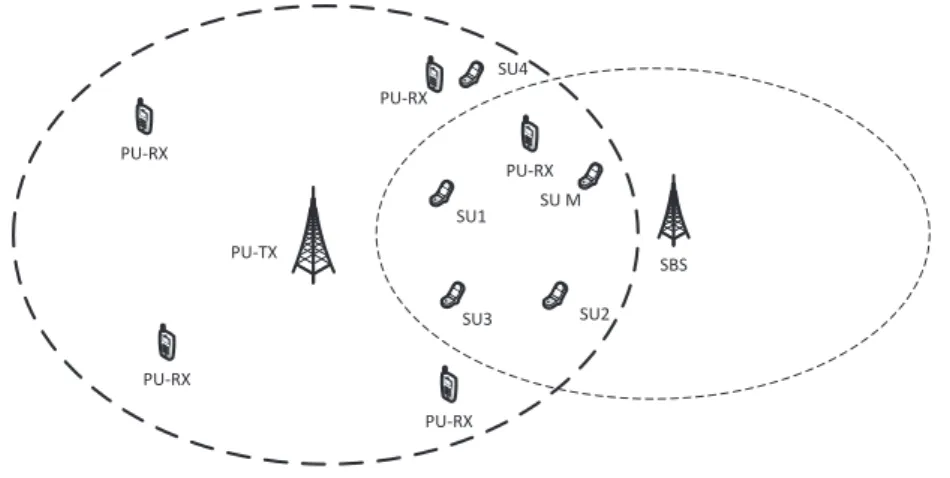
3.3 Cognitive radio network of primary and secondary users. 51

(21)

LIST OF FIGURES xvi

3.4 ROC performance comparison showing EV based SVM and ED based SVM schemes under diﬀerentSN R range, number of antenna, M = 5, and number of samples,Ns= 1000 . 64

3.5 ROC performance comparison showing EV based SVM and ED based SVM schemes with diﬀerent number of antenna,

M,SN R = -18dB, and number of samples, Ns= 1000 . 65

3.6 ROC performance comparison showing EV based SVM and ED based SVM schemes with diﬀerent number of samples,

Ns, number of antenna,M = 5, andSN R = -20 dB . 65

3.7 Performance comparison between EV based SVM and ED based SVM schemes showing probability of detection and prob-ability of false alarm versus SN R, with samples number, Ns

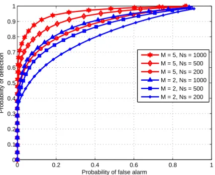
= 1000, number of antenna,M = 3, 5 and 8. 66 3.8 ROC curves for CSVM with number of PU = 2, number of

antennas, M = 2 and 5, number of samples, Ns = 500,1000

atSN R = -15dB. 69

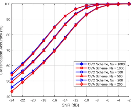
3.9 Comparison between OVO and OVA coding Schemes with number of PU = 2, number of sensors, M = 5, number of samples, Ns = 200, 500 and 1000. 70

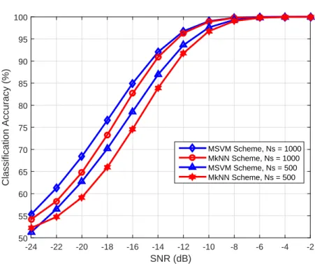
3.10 Comparison between OVO-MkNN and OVO-MSVM, with num-ber of PU = 2, numnum-ber of sensors, M = 5, numnum-ber of samples,

Ns = 500 and 1000. 71

3.11 Comparison between OVO-MkNN and OVO-MSVM, with num-ber of PU = 2, numnum-ber of sensors, M = 5 at SNR = -10 dB,

(22)

LIST OF FIGURES xvii

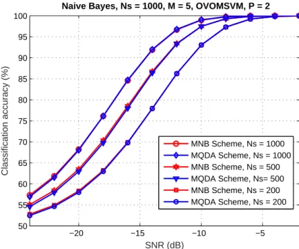
3.12 Comparison between OVO-MNB and OVO-MQDA, with num-ber of PU = 2, numnum-ber of sensors, M = 5, numnum-ber of samples,

Ns = 200, 500 and 1000. 72

4.1 Cooperative spectrum sensing network of single PU and

mul-tiple SUs. 77

4.2 Constellation plot showing clustering performance of K-means algorithm, SN R = -13dB, number of PU, P = 1, number of sensors, M = 2, number of samples,N s= 2000. 91 4.3 ROC curves showing the sensing performance of theK-means

algorithm, number of PU,P = 1, number of sensors, M = 2, number of samples,N s= 1000 and 2000,SN R = -13 dB and

-15 dB. 92

4.4 Constellation plot showing probability distribution of mixture components, SN R = -13dB, number of PU, P = 1, number of sensors, M = 2, number of samples,N s = 2000. 93 4.5 Constellation plot showing the mixture components’ posterior

probability derived from the E-M algorithm, number of PU,

P = 1, number of sensors, M = 2, number of samples, N s=

2000, SN R = -13 dB . 94

4.6 Constellation plot showing the clustering capability of the E-M algorithm, number of PU, P = 1, number of sensors,M = 2, number of samples,N s= 2000, SN R = -13 dB. 94 4.7 ROC curves showing the sensing performance of the E-M

al-gorithm, number of PU, P = 1, number of sensors, M = 2, number of samples,N s= 1000 and 2000,SN R = -13 dB and

(23)

LIST OF FIGURES xviii

4.8 A spectrum sensing system of a primary user and mobile

sec-ondary users networks. 97

4.9 Time varying channel gain (CG) tracked at [a] SN R = 5 dB

and [b] SN R = 20dB. 106

4.10 Mean square error performance of the AR-1 based Kalman ﬁlter at normalized Doppler frequency = 1e-3, tracking dura-tion,Ts = 100, 500 and 1000 symbols. 107

4.11 Average probabilities of detection and false alarm vs SN R, tracking SN R = 5 dB, number of samples, Ns = 1000 and

2000, tracking duration = 1000 symbols. 108 4.12 Average probabilities of detection and false alarm vs SN R,

trackingSN R= 5dB, number of samples,Ns = 2000,

track-ing duration = 1000 symbols. 109

5.1 Constellation plot of three Gaussian components blindly iden-tiﬁed, number of PUs,P = 2, number of samples, Ns= 3000,

the number of antennas, M = 3,SNR = -12dB. 138 5.2 Probabilities of detection and false alarm versusSNRwithNs

= 5000, 7000, 10000, P = 1, M = 3. 139 5.3 ROC curves showing the performance of VBGMM algorithm,

at SNR = -15 dB, Ns = 1000, 1500, 2000 and 2500, P = 1,

M = 2. 139

5.4 Clustering accuracy versus SNR,P = 2,M = 3, Ns = 2000

and 5000. 140

5.5 Probabilities of detection and false alarm versus SNR with diﬀerentNs,P = 1,M = 3, showing comparison between VB

(24)

LIST OF FIGURES xix

6.1 ROC performance comparison between beamformer based and non-beamformer based SVM schemes under diﬀerent SN R, number of PU, P = 1 and number of samples, N s= 500. 157 6.2 ROC performance comparison between beamformer based and

non-beamformer based SVM schemes with diﬀerent number of samples N s, andSN R = -20 dB. 157 6.3 Performance comparison between beamformer based and

non-beamformer based SVM schemes showing probabilities of de-tection and false alarm versus SN R, with diﬀerent sample

number,N s. 160

6.4 Performance comparison between OVO and OVA ECOC MSVM schemes under non-overlapping transmission scenario with dif-ferent number of samples N s, and number of PU,P = 2. 160 6.5 Performance comparison of OVO MSVM, MIMSVM and OVO

NBMSVM schemes under LOS transmission scenario with dif-ferent number of samples N s, and number of PU,P = 2. 161 6.6 Performance comparison of MSVM, MIMSVM and

OVO-NBMSVM schemes under non-overlapping reﬂection scenario with diﬀerent number of samples N s, and number of PU,P

= 2. 161

6.7 Performance comparison of OVO MSVM, MIMSVM and OVO NBMSVM schemes under overlapping reﬂection scenario with diﬀerent number of samples N s, and number of PU,P = 2. 162 6.8 Performance comparison between OVO ECOC and DAG based

MSVM under non-overlapping reﬂection scenario with diﬀer-ent number of samplesN s, and number of PU,P = 2. 163

(25)

LIST OF FIGURES xx

6.9 Performance comparison of OVO based MSVM and MkNN techniques with diﬀerent number of samples N s, number of neighbor = 5, and number of PU,P = 2. 165

(26)

Chapter 1

INTRODUCTION

1.1 Basic Problem

In many countries around the globe, the electromagnetic spectrum assigned to wireless networks and services is managed by governmental regulatory bodies. For example, there is the European Telecommunications Standards Institute in Europe (ETSI) and the Federal Communications Commissions (FCC) in United States. These governing bodies are saddled with the re-sponsibility of allocating spectral frequency blocks to specific groups or com-panies. More often than not, the allocation process involves (i) partition-ing of the spectrum into distinct bands, with each band spannpartition-ing across a range of frequencies; (ii) assigning specific communication services to spe-cific bands, and (iii) deciding the licensee for each band who usually is given the exclusive right over the use of the allocated frequency band. Since the licensee reserves the right over the assigned spectrum, it can easily manage interference and the quality of service (QoS) among its users [3].

In the last one decade, there has been unprecedented concern over the static manner in which the natural frequency spectrum is being allocated. This concern is further being heightened by the ever increasing demand for higher data rates as wireless communication technology advances from voice only communications to data intensive multimedia and interactive services now being ubiquitously deployed [4]. In order to meet the challenge of spec-trum crisis thus created, a paradigm shift from the hitherto, command and 1

(27)

Section 1.1. Basic Problem 2

control manner of frequency allocation to dynamic spectrum access has be-come imperative. Interestingly, going by the current allocation technique, spectrum occupancy measurements have shown that most of the allocated spectral bands are often underutilized. For example, studies conducted in the United States have revealed that in most locations, only 15% of spec-trum is used. More specifically, a field specspec-trum measurement taken in New York City showed that the maximum total spectrum occupancy for bands from 30MHz to 3GHz is only 13.1 % [4], [5]. Similar result was also obtained in the most crowded area of downtown Washington, D.C., where occupancy of less than 35 % is recorded for the radio spectrum below 3 GHz [4]. In addition, it is a well known fact that spectrum usage also varies significantly at various time, frequency and geographic locations [6].

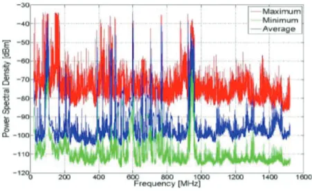
Figure 1.1. Maximum, minimum, and average received power spectral density in the frequency band 20 - 1,520 MHz with a 200-kHz resolution bandwidth of the receiver. Outdoor location: on top of 10 - storey building in Aachen, Germany [1].

Figure 1.1 shows the maximum, minimum and average spectrum us-age in an outdoor environment at a typical location in Aachen, Germany, demonstrating enormous variations of interference power. In Figure 1.2, it is further shown that in an indoor environment, the spectrum usage is even

(28)

Section 1.2. Cognitive Radio Technology 3

Figure 1.2. Average received power spectral density in the frequency band 20 - 1,520 MHz with a 200-kHz resolution bandwidth of the receiver. Indoor location: inside an oﬃce building in Aachen, Ger-many [1].

smaller, and on average, mostly thermal noise is present. From the forego-ing, it is very clear that radically new approaches are required for better utilization of spectrum, especially in the face of the current unprecedented level of demand for spectrum access.

1.2 Cognitive Radio Technology

Cognitive radio (CR) is an emerging technology that can successfully deal with the growing demand and scarcity of the wireless spectrum [7–11]. It is a paradigm of wireless communication in which an intelligent wireless sys-tem utilizes information about the radio environment to adapt its operating characteristics in order to ensure reliable communication and eﬃcient spec-trum utilization. Recently, several IEEE 802 standards for wireless systems have considered cognitive radio systems such as IEEE 802.22 standard [12] and IEEE 802.18 standard [13].

(29)

users popularly referred to as the secondary users (SUs) to access licensed spectrum bands without causing harmful interference to the service of the licensed users otherwise referred to as primary users (PUs) [8]. In the fol-lowing sub-section, the basic approaches that facilitate the implementation of dynamic spectrum access in CR networks will be described.

1.2.1 Cognitive Radio Network Paradigms

There are three main techniques that are being considered for cognitive spec-trum sharing. These are the overlay, underlay and interweave techniques [3]. In the overlay approach, the SUs coexist with PUs based on the assumption that the knowledge of the PU’s codebook and message is available to the SUs. This knowledge can be used to either cancel or reduce the interference caused by the PUs’ transmission to the SUs thorough sophisticated signal processing techniques such as dirty paper coding (DPC) [3]. In order to offset the interference caused by the SUs’ transmissions to the PUs, the SUs can split up their transmission power and use part of it to relay the PUs’ signals to the intended primary receiver. This will ensure that the PUs’ sig-nal is received with desired sigsig-nal-to-noise ratio (SN R). At the same time, the SUs can use the remaining transmit power for their own communication. Hence, both the PUs and the SUs benefit by allowing SUs spectrum access. In the underlay approach, the SUs access the licensed spectrum without causing harmful interference to PUs’ communications. This requires the SUs to ensure that interference leakage to the primary users is below an acceptable threshold. One way the SUs can meet the interference constraint is by employing multiple antennas to steer their beams away from the PUs. Alternatively, the SUs may employ spread spectrum technique whereby the transmitted signal is spread across a wide bandwidth such that the power level is below the noise floor. At the SU receivers, the signals may then be recovered through de-spreading. It should be noted that since the constraint

(30)

on the interference is somewhat restrictive under the underlay method, the transmissions by the SUs may be limited to short range communications. The underlay approach is illustrated in Fig. 1.3.

Figure 1.3. Underlay spectrum paradigm. Green and red represent the spectrum occupied by the primary users and the secondary users respectively.

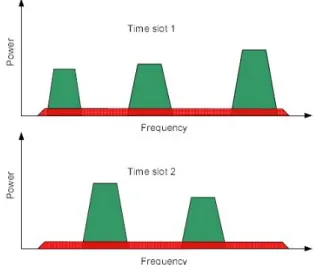
The third cognitive technique for spectrum sharing is the interweave method shown in Fig. 1.4, in which case the SUs are permitted to access the licensed band in an opportunistic manner, i.e. only when and where

it is not being used. The absence of an active PU in a band indicates that its allocated channel is idle and available for use by SUs while the PU’s presence indicates otherwise. An idle or unused channel is often described as a spectrum hole or white space [3], [8]. However, since the PUs have priorities to use the bands, the SUs need to continuously monitor the activities of the PU to avoid causing intolerable interference to the PU’s service. To meet this requirement, once granted permission to utilize unused spectrum, the SU must be alert to detect the reappearance of the PU and once detected, it should vacate the spectrum within the shortest possible, permissible time to minimize the interference caused to the licensed user.

(31)

funda-Section 1.2. Cognitive Radio Technology 6

Figure 1.4. Interweave spectrum scheme. Green and red represent the spectrum occupied by the primary users and secondary users re-spectively.

mental task that is crucial to the successful implementation of the interweave cognitive radio system is detecting the presence or absence of the PU. This is usually referred to as spectrum sensing [4]. Put in another way, without spectrum sensing, no opportunistic use of the spectrum hole by SUs can take place. To summarize, the interweave cognitive radio can be described as an intelligent wireless communication system which requires the SUs to contin-uously monitor the activities of the PUs and intelligently detect availability of spectrum holes in order to take advantage of idle band towards achieving eﬃcient utilization of radio spectrum resources.

There is no gainsaying that identifying spectrum holes in the absence of cooperation between primary and secondary networks is a very challenging task [14]. Nevertheless, unlike in overlay and underlay methods, the inter-weave scheme is non-invasive and there is no restriction in terms of transmit power and coverage, thus oﬀering tremendous advantages in terms of high data rate and achievable QoS for the SUs, especially so in the event that the licensed band is idle for a reasonably prolonged period of time. Hence, the rest of this thesis is aimed at developing intelligent sensing techniques for

(32)

Section 1.3. Motivation for Machine Learning Techniques 7

opportunistic spectrum access.

1.3 Motivation for Machine Learning Techniques

In order for cognitive devices to be really cognizant of the changes in the activities taking place in their radio frequency (RF) environment, it is im-perative that they be equipped with both learning and reasoning function-alities. Little wonder then, that Simon Haykin in [8] envisioned CRs to be brain-empowered wireless devices that are speciﬁcally deigned to improve the utilization of the electromagnetic spectrum. These capabilities can eas-ily be embedded in a cognitive engine which coordinates the actions of the CR by making use of machine learning∗ algorithms. In wireless communi-cation and dynamic spectrum access in particular, several parameters and policies need to be adjusted simultaneously; these include transmit power, coding scheme, modulation scheme, sensing algorithm, communication pro-tocol, sensing policy, etc. No simple formula may be able to determine these parameters simultaneously due to the complex interactions among these fac-tors and their impact on the RF environment. Learning methods can be successfully applied to allow eﬃcient adaption of the CRs to their environ-ment, yet without the complete knowledge of the dependence among these parameters [16].

In general, learning methods can be classified as supervised, semi-supervised and unsupervised [17]. Supervised algorithms require training and creating decision models using labeled data. On the other hand, semi supervised tech-niques do not require labeled data, however, the knowledge of the statistical characteristics of the distribution which the training data follows may be required. The unsupervised classification algorithms do not require labeled training data and can be classified as either parametric or non-parametric.

∗_{Machine learning is a bio-inspired ﬁeld of study which can be described as “the}

(33)

Section 1.4. Structure of Thesis and Contributions 8

While the supervised and semi-supervised techniques can generally be used in familiar or known environments with prior knowledge about the charac-teristics of the environment, these knowledge may not be required for the implementation of unsupervised learning, thus lending itself readily to au-tonomous signal detection in alien radio environments. It is particularly of interest to know that these learning techniques have been applied in solving many data mining problems involving classiﬁcation. It is opined that they can equally be successfully developed into algorithms for proﬀering solution to our spectrum sensing problem.

1.4 Structure of Thesis and Contributions

To facilitate the understanding of this thesis and its contributions, the struc-ture is summarized as follows:

In Chapter 1, the current frequency allocation method as well as the spectrum scarcity and under-utilization problems is ﬁrst introduced. This is followed by a general description of the CR technology as a widely acceptable panacea. Further, the various possible approaches for implementing CR systems are described and spectrum sensing is highlighted as a fundamental process crucial to the successful implementation of CR. In addition, the motivation for choosing machine learning techniques as the basis for the various solutions that are proposed in this thesis is provided. The chapter concludes with an outline of the thesis structure and its contributions.

In Chapter 2, a brief introduction of the spectrum sensing problem for-mulation is presented. This is followed by a consideration of the existing local techniques for spectrum sensing that have been proposed for use by stand alone sensor nodes. The techniques described cover both blind and semi blind methods such as the matched ﬁltering method, energy detection based methods and the hybrid schemes. The cooperative sensing method

(34)

for mitigating the eﬀects of channel imperfections and improving detection performance is also brieﬂy described.

In Chapter 3, supervised classiﬁers based algorithms are presented and the performance is evaluated in terms of spectrum sensing capability using the energy based features. Next, a novel eigenvalue based feature is proposed and its capability to improve the performance of the support vector machine (SVM) algorithms under multi-antenna considerations is demonstrated. Fur-thermore, spectrum sensing under multiple PU scenarios is considered and to facilitate spatio-temporal spectrum hole detection, the conventional, binary hypothesis spectrum sensing problem is re-formulated as a multiple signal detection problem comprising multiple system states. In addition, the perfor-mance evaluation of the multi-class error correcting output codes (ECOC) based SVM algorithms is presented using both the energy and eigenvalue based features. The simulation results indicate that the proposed detec-tors are robust to both temporal and joint spatio-temporal spectrum hole detection.

In Chapter 4, two semi-supervised parametric classifier algorithms are presented for use in sensing scenarios where only partial information about the PUs’ network is available to the SUs. With these algorithms in mind, the problem of spectrum sensing in mobile SUs is further considered and a tech-nique for enhancing the classifiers’ performance is proposed. In particular, spectrum sensing under slow fading Rayleigh channel conditions due to the mobility of SUs in the presence of scatterers and the resulting performance degradation is of concern. To address this problem, the use of Kalman filter based channel estimation technique for tracking the temporally correlated slow fading channel is proposed to aid the classifiers to update the decision boundary in real time.

In Chapter 5, a fully Bayesian, soft assignment unsupervised classiﬁca-tion algorithms based on the variaclassiﬁca-tional learning framework is presented.

(35)

This technique overcomes some of the limitations of supervised and semi-supervised algorithms in terms of the amount of information about the PU network that is required for optimal performance. In particular, the problem of blindly estimating the number of active transmitters and the statistical pa-rameters that characterize the distribution of the signals from the unknown number of transmitters is considered. The inference problem is approached as a blind source separation problem. The proposed algorithm is shown to be useful for simultaneously monitoring the activities of multiple PU across multiple sub-bands and for autonomous spectrum sensing in alien radio en-vironments where the prior knowledge of the exact number of sources is not available at the SU.

The performance of classiﬁcation algorithms depends to a large extent on the quality of the training and prediction data used. In harmony with this thought, in Chapter 6 a novel, beamformer based pre-processing tech-nique for feature realization is proposed towards improving the quality of our features and hence, the performance of our classiﬁer based sensing algo-rithms particularly in multi-antenna CR networks. Using this novel feature technique, the ECOC based multi-class SVM algorithms is re-investigated and a multiple independent model (MIM) alternative is provided for solving the multi-class spectrum sensing problem. Simulation results are provided to demonstrate the superiority of the proposed methods over previously pro-posed alternatives.

Finally, in Chapter 7 this thesis is concluded with a summary of its contributions and suggestions for possible future research directions.

(36)

Chapter 2

REVIEW OF RELEVANT

LITERATURE

2.1 Introduction

Spectrum sensing problem is usually approached in one of two ways. These are the physical layer (PHY) and the media access control layer (MAC) ap-proaches [18]. The PHY layer based spectrum sensing is the most common and typically focuses on the detection of instantaneous primary user sig-nals. The MAC layer approach on the other hand is essentially a resource allocation issue, where the concern is how to handle the problem of schedul-ing when the channel of interest is best sensed. It also involves addressschedul-ing estimation problem where the desire is to extract the statistical properties of the randomly varying PU-SU channel based on the assumption that the physical layer sensing provides suﬃciently accurate results on instantaneous channel availability [18]. In this chapter, attention is focused primarily on the physical layer approach and a review of the most common and relevant methods is presented.

2.2 Local Spectrum Sensing Techniques

As highlighted in the opening chapter of this thesis, the goal in performing spectrum sensing is to identify the availability of spectrum holes while also 11

(37)

Section 2.2. Local Spectrum Sensing Techniques 12

protecting the PU terminals from harmful interference. In general, from the perspective of local spectrum sensing involving individual SUs, if the instantaneous signal received at the SU terminal is represented asx(n), the spectrum sensing problem can be formulated as a binary hypothesis testing of the form x(n) =        η(n), under H0 ϕ(n)s(n) +η(n), under H1 (2.2.1)

where H0 denotes the hypothesis that the PU is absent and H1 denotes

the hypothesis that the PU signal is present in the band of interest. Fur-thermore, η(n) is the additive white Gaussian noise (AWGN), ϕ(n) is the gain coeﬃcient of the channel between the PU and the SU and s(n) is the transmitted primary signal. To solve the signal detection problem in (2.2.1), diﬀerent techniques have been proposed which are described as follows.

2.2.1 Matched Filtering Detection Method

The match ﬁltering (MF) technique also known as coherent detection is a method that requires the SU to have perfect knowledge of the PU signal and the channel between PU and SU so that with accurate synchronization, the received signal can be correlated with the known signal to determine the presence or absence of the PU [19]. The MF method has been described as the optimal detection method because it maximizes theSN Rin the presence of additive noise and also minimizes the decision errors [10], [20]. If the primary transmitted signal, s(n), is deterministic and known a priori, the matched ﬁlter correlates the known signals(n) with the received, unknown signalx(n), and the decision is made using the expression [21], [22]

Υ(x), Ns ∑ n=1 x(n)s∗(n)H≷1 H0 θt (2.2.2)

(38)

where Υ(x) is the test statistic which is assumed to be normally distributed under both hypothesesH0 andH1, i.e.,

Υ(x)∼        N(0, Nsσs2ση2), under H0 N(Nsσ2s, Nsσs2ση2), under H1 (2.2.3)

σ_s2 = ∥s∥2/Ns, represents the average primary signal power while θt is the

decision threshold andNsis the number of samples used to perform

correla-tion. The probability of false alarm (P f a) and probability of detection (P d) are given by Pf a=Q ( θt σησs √ Ns ) (2.2.4) and Pd=Q (θt−Nsσs2 σησs √ Ns ) (2.2.5) where Q(z) = √1 2π ∫+∞ z e− τ2

2 dτ is the tail probability of a zero-mean unit variance Gaussian random variable, also known as Q-function. If we let

SN R , σ2s

σ2

η =

∥s∥2

Nsσ2η, then the required number of samples, Ns, to achieve

an operating point in terms ofPf a and Pd can be determined by combining

(2.2.4) and (2.2.5), as

Ns= [Q−1(Pf a)−Q−1(Pd)]2SN R−1 (2.2.6)

The main advantage of MFs is that within a short time, a certainP dorP f a

is achievable compared to the other proposed methods [4]. However, in a situation where the signal transmitted by the PU is unknown to the SU, the MF technique cannot be used. Also, it is not very useful when synchroniza-tion becomes very diﬃcult especially at low SN R. Furthermore, owing to the fact that the CR needs receiver for all types of signal, the implementation complexity of the sensing unit would be impractically large. Moreover, the power consumption of the MF is also considerably high since for detection,

(39)

various receiver algorithms need to be executed [4]. Nevertheless, the MF can be very useful in applications where the pilot signal of the primary signal is known [23].

2.2.2 Cyclostationary Feature Detection Method

The cyclostationary detector (CD) is one of the feature detectors that take the advantage of the fact that unique patterns that are peculiar to a spe-ciﬁc signal can be used to detect its presence or absence. Most primary signals are modulated sinusoidal carriers, have certain symbol periods, or have cyclic preﬁxes which constitute built in periodicity. Such periodicity can distinguish the PU signal from other modulated signals and background noise, even at a very low SN R [21, 23, 24]. Mathematically, cyclostationary detection can be realized by analyzing the cyclic autocorrelation function (CAF) of the received signal or its two-dimensional spectrum correlation function (SCF) [23]. The modulated signal s(n), can be characterized as a wide sense second order cyclostationary process because both its mean and autocorrelation exhibit periodicity [21]. If we letµs=E[s(n)] andRs(n1, n2)

=E[s(n1)s∗(n2)], then,∀n,n1 andn2, it holds thatµs(n) =µs(n+T0) and Rs(n1, n2) = Rs(n1+T0, n2+T0), where T0 > 0 is a fundamental period.

For a wide-sense second order cyclo-stationary process, having a non-zero cyclic frequency (ω̸= 0), the cyclic autocorrelation function is deﬁned as

Rω_s(l),E[s(n)s∗(n+l)e−2πωn]. (2.2.7) Equation (2.2.7) can be described as

Rω_s(l) =        ﬁnite, if ω = _Tm 0 0, otherwise (2.2.8)

(40)

for any non-zero integer m. Thus, for a cyclostationary process {s(n)},

∃ω ̸= 0 such that Rω_s(l) ̸= 0 for some value of l. In the frequency domain, the corresponding representation ofR_sω(l), known as the spectral correlation function can be obtained by using the discrete time Fourier transformation. This can be expressed as

sω_s(eiς) =

+∞

∑

l=−∞

Rω_s(l)e−iςl, (2.2.9) where ς ∈ [−π, π] is the digital frequency corresponding to the sampling rate, fs. The binary hypotheses test for the cyclostationary detection can

then be written as sω_x(eiς) =        sω_η(eiς), under H0 sω

s(eiς) +sωη(eiς), under H1.

(2.2.10)

Unlike the transmitted primary signal, the noiseη(n) is in generalnot periodic

such that sω_η(eiς) = 0, ∀ω ̸= 0. For Ns available measurements of the

re-ceived signal, atς = 2_Dπg, the spectral correlation function can be obtained as ˆsω_x(g) = 1 Ns Ns ∑ n=1 xD(n, g+ gω 2 )x ∗ D(n, g− gω 2 ), (2.2.11) where xD(n, g) = 1 √ D n+_∑D₂−1 d=n−D 2 x(d)e−i2πgdD (2.2.12)

is the D-point discrete Fourier transform around the n-th sample of the received signal, and gω = ωD_f_s is known as the index of the frequency bin

corresponding to the cyclic frequency, ω. Suppose that for a single cycle (sc) the ideal spectral correlation function,sω_s(g), is known a priori, the test

(41)

statistic for the cyclostationary detection is given by [21]

Υsc(x) = D_∑−1 g=0 [ ˆ sω_x(g)][sω_s(g)]∗ H1 ≷ H0 θt, (2.2.13)

and for a multicycle (mc) detector, the test statistics is

Υsc(x) = ∑ ω D∑−1 g=0 [ ˆ sω_x(g)][s_sω(g)]∗H≷1 H0 θt. (2.2.14)

where the sum is taken over all ω’s for which sω

s(g) is not identically zero

and the vectors, x and s can be deﬁned as: x , [x(1),· · · , x(Ns)]T and

s , [s(1),· · · , s(Ns)]T. While the CD is well coveted for its robustness in

the presence of noise uncertainty and low SN R, its drawbacks include the requirement of having a priori knowledge of the PU signal characteristics which may not be practical for many frequency reuse applications, long sensing time and high computational complexity [10], [18]. The detector is suitable when the period,T0 of the primary signal is known [23].

2.2.3 Energy Detection Method

The energy detection (ED), also known as radiometry or periodogram is the most common and most investigated spectrum sensing method because of its low computational and implementation complexity [4, 19, 25–28]. In the ED method, the a priori knowledge of the characteristics of the PU signal is not required and as such, it is a non-coherent technique that can be used to detect the presence or absence of the primary signal based on the sensed energy. The decision is made by comparing the mean squared accumulation of the received signal strength in a certain time interval to a pre-determined threshold [29]. Like the other spectrum sensing techniques, the goal is to decide between the two hypotheses, H0 and H1. The decision rule in this

(42)

Section 2.2. Local Spectrum Sensing Techniques 17 case is given by Υ(x) = Ns ∑ n=1 |x(n)|2 H≷1 H0 θt, (2.2.15)

where Υ(x) is the test statistics andθtis the corresponding decision

thresh-old. When the PU is absent, Υ(x) obeys a central Chi-square distribu-tion with Ns degrees of freedom; otherwise, Υ(x) obeys a non-central

Chi-distribution with Ns degrees of freedom and a non-centrality parameter λ

=σ2

sNs [27]. IfNs is large enough (Ns>20) [30], due to central limit

the-orem, Υ(x) is asymptotically normally distributed, hence the statistics can be modeled as Υ(x)∼        N(Nsσ2η,2Nsση4), H0 N(Nsσ2η+Nsσ2s,2Nsσ4η+ 4Nsσ2ησ2s), H1. (2.2.16)

The Pf a, and thePd, can be approximated as [21]

Pf a =Q (θt−Nsση2 σ2 η √ 2Ns ) (2.2.17) and Pd=Q ( θt−Nsση2−Nsσ2s ση √ 2Nsση2+ 4Nsσs2 ) (2.2.18)

respectively. Using (2.2.17) and (2.2.18), the number of samples,Nsrequired

to attain desired values ofPf a and Pd is given by

Ns = 2[Q−1(Pf a)−Q−1(Pd)

√

1 + 2SN R]2SN R−2. (2.2.19)

The ED is very practical since no information about the primary user is required. However, the uncertainty of noise degrades its performance [20]. Besides, below an SN R threshold referred to as the SN R wall, a reliable detection cannot be achieved by increasing the sensing duration [19], [31]. Moreover, the energy detector cannot distinguish the PU signal from the

(43)

noise and other interference signals, which may lead to a high false alarm probability.

2.2.4 Eigenvalue Based Detection Methods

The eigenvalue-based detection has been proposed for use in spectrum sens-ing in a multi-antenna system [19]. The technique is found to achieve both highPdand lowPf a without requiring much information about the PU

sig-nal and noise power. In the existing methods, the expression for the decision threshold,PdandPf aare calculated based on the asymptotical distributions

of the eigenvalues [32]. The eigenvalue of the signal received at the SU dur-ing the sensdur-ing interval is derived as follows. Let us suppose that the SU is equipped with M antennas and that the PU is transmitting, the M×1 observation vector at the receiver can be deﬁned as

x(n),[x1(n), x2(n), ..., xM(n)]T (2.2.20)

hp(n),[h1,p(n), h2,p(n), ..., hM,p(n)]T (2.2.21)

η(n),[η1(n), η2(n), ..., ηM(n)]T . (2.2.22)

If we assume that there are P transmitting PUs, the received signal vector can be expressed as x(n) = P ∑ p=1 Kp ∑ k=0 hp(k)sp(n−k) +η(n), n= 0,1,2· · · (2.2.23)

where the vectorhp(n) represents the channel gain betweenP Up and all the

antennas of the SU while Kp is the order of the channel between P Up and

each antenna of the SU. Assuming we also consider N consecutive samples of the transmitted PU signal, the corresponding signal and noise vectors can

(44)

Section 2.2. Local Spectrum Sensing Techniques 19 be deﬁned as xN(n),[xT(n),xT(n−1), ...,xT(n−N+ 1)]T sN(n),[sT1(n),sT2(n), ...,sTP(n)]T η_N(n),[ηT(n),ηT(n−1), ...,ηT(n−N + 1)]T (2.2.24)

where sT_p(n) ,[sp(n), sp(n−1),· · · , sp(n−Kp−N + 1)] and N is known

as the smoothing factor [32], [33]. In matrix form, the received signal model can be expressed as

xN(n) =HsN(n) +ηN(n) (2.2.25)

where the matrixH, of orderM N×(K+NP),K=∑P_p₌₁Kp is deﬁned as

H,[H1,H2,· · · ,HP], (2.2.26) where Hp ,       hp(0) · · · · · · hp(Kp) · · · 0 . .. . .. 0 · · · hp(0) · · · · · · hp(Kp)      , (2.2.27)

and Hp is a M N ×(Kp+N) matrix. The statistical covariance matrix of

the received signals can then be written as

Rx =HRsHH+σ2nIM N, (2.2.28)

where Rs =E[SN(n)SHN(n)], IM N is the identity matrix of orderM N and

(.)H denotes Hermitian transpose. However, in practice, we have only ﬁnite number of samples, denoted asNs. This means that instead of the statistical

(45)

matrix which can be written as [32]

Rs(Ns), 1 Ns L−∑2+Ns n=L−1 x(n)x†(n). (2.2.29)

Based on the matrix in (2.2.29), two blind spectrum sensing algorithms have been proposed [32]. The ﬁrst one is called the maximum-minimum eigenvalue (MME) detection algorithm where as the name suggests, the maximum and minimum eigenvalue of the matrix denoted asλmax and λmin are computed

and the test statistics for deciding the presence or absence of the PU is the ratioλmax toλmin. The decision rule is given as

Υ(Rs(Ns)) = λmax λmin H1 ≷ H0 θt (2.2.30)

where θt > 1 is a threshold. The second sensing algorithm is known as the

energy with minimum eigenvalue (EME) detection method. In this case, test statistics for detection is the ratio of energy to minimum eigenvalue, i.e. T(Ns)

λmin where the energy,T(Ns), of the received signals in this instance is

computed as [32] T(Ns) = 1 M Ns M ∑ m=1 N∑s−1 n=0 |xm(n)|2. (2.2.31)

The decision rule is therefore given as

Υ(Rs(Ns)) = T(Ns) λmin H1 ≷ H0 θt (2.2.32)

whereθt is as deﬁned for the MME method.

2.2.5 Covariance Based Method

In general, the statistical covariance matrices or autocorrelations of signal and noise are diﬀerent. Using sample covariance matrix computed over Ns,

(46)

Zeng and Liang [34], proposed to use the diﬀerence to perform spectrum sensing under the assumption that the PU’s signal is correlated. If we denote the statistical covariance matrix asRx, and the sample autocorrelations of

the received signal is computed as

r(l) = 1

Ns N∑s−1

n=0

x(n)x(n−l), l= 0,1, ..., N −1, (2.2.33)

where N is known as the smoothing factor. The sample covariance matrix, ˆ

Rx(Ns), which approximates the statistical covariance matrix can be deﬁned

as ˆ Rx(Ns),          r(0) r(1) · · · r(N−1) r(1) r(0) · · · r(N−2) .. . ... . .. ... r(N−1) r(N −2) · · · r(0)          . (2.2.34)

Under H0, the oﬀ-diagonal elements of ˆRx(Ns) are theoretically zero since

the noise is usually assumed to be uncorrelated. The diagonal elements also contain the noise power. On the other hand, underH1, the oﬀ-diagonal

elements should be non-zeros due to the correlatedness of the primary signal. In this case, there are two terms of interest and they are computed as

T1(Ns) = 1 N L ∑ i N ∑ j |rij(Ns)| (2.2.35) and T2(Ns) = 1 N N ∑ i |rii(Ns)| (2.2.36)

whererij(Ns) are the elements of the matrix in (2.2.34). The test statistics

for determining the presence or absence of PU is given by

Υ( ˆRx(Ns)) = T1(Ns) T2(Ns) H1 ≷ H0 θt (2.2.37)

(47)

whereθt is an appropriate threshold.

2.2.6 Wavelet Method

The wavelet transform is a powerful mathematical tool for analyzing singu-larities and edges [35]. In wavelet method based spectrum sensing schemes, the spectrum of interest is usually decomposed as a train of consecutive fre-quency sub-bands and wavelet transform is then used to detect irregularities in these bands. An important characteristic of the power spectral density (PSD) is that it is relatively smooth within the sub-bands and possesses irregularities at the edges between two neighboring sub-bands. So, wavelet transform carries information about the locations of these frequencies and the PSD of the sub-bands. Vacant frequency bands can be obtained through the detection of thesingularitiesin the PSD of the signal observed, by per-forming the wavelet transform of its PSD [20].

The process for the wavelet detection methods can be described as fol-lows [35]. First, let us assume that we have a total of B Hz spread across the frequency range [f0, fN] for a wideband wireless system. Further, we

assume that the entire band is divided into N bands where each sub-band is occupied by individual PU and all sub-sub-bands are being simulta-neously monitored. The sensing task involves detecting the locations and PSD within each sub-band. Let us suppose that the sub-bands lie consec-utively within [f0, fN], such that there are frequency boundaries located at

f0 < f1 < · · ·fN. The n-th band may thus be deﬁned by Bn : {f ∈ Bn :

fn−1 ≤ f < fn}, n = 1,2,· · · , N. Under H1, the normalized, unknown

power shape within each band, Bn is denoted by Sn(f) and satisﬁes the

conditions [35]

Sn(f) = 0, ∀f /∈Bn; (2.2.38)

∫ fn

fn−1

(48)

If it is assumed that the PSD within each band, Bn is smooth and almost

ﬂat but exhibits discontinuities from its neighboring bandsBn−1 andBn+1,

such that irregularities in PSD appears only at the edges of the bands,Sn(f)

may be approximated as Sn(f) =        1, ∀f ∈Bn. 0, ∀f /∈Bn. (2.2.40)

The PSD of the observed time domain signal, x(t), can then be written as

Sx(f) = N ∑ n=1 ¯ α2_nSn(f) +Sw(f), f ∈[f0, fN] (2.2.41)

where it is assumed that the noise is additive and white with two sided PSD,Sw(f) = N₂0,∀f, and ¯αn2 indicates then-th band signal power density.

Furthermore, the corresponding time domain equivalent of (2.2.41) can be written as x(t) = N ∑ n=1 ¯ αnpn(t) +w(t) (2.2.42)

where Sn(f) is the signal spectrum of pn(t) and w(t) is the additive noise

whose PSD isSw(f). Furthermore, if we assume a pulse shaper,ht of

band-width fn−fn−1 , and the center frequency is denoted by fc,n = fn−1₂+fn,

the spectral shape, Sn(f) is proportional to |F{ht}|2, where F{.} denotes

the Fourier transform (FT). It is desired that x(t) with PSD Sx(f) be used

to estimate {fn}Nn=1−1 and {α¯2n}Nn=1, which characterize the wideband

spec-tral environment under consideration. If we letκ(f) be a wavelet smoothing function, for example, the Gaussian function with a compact support,g van-ishing moments andgtimes continuously diﬀerentiable, the dilation of κ(f) by a scale factors is given by [35]

κs(f) =

1

sκ( f

(49)

where for dyadic scales, s takes values from powers of 2, i.e. s = 2j, j = 1,· · · , J. The continuous wavelet transform (CWT) of Sx(f) in (2.2.41) is

given by

WsSx(f) =Sx∗κs(f) (2.2.44)

where ∗ denotes the convolution operation. It is worth noting here that CWT in (2.2.44) is implemented in the frequency domain and Sx(f) is

re-lated to x(t) via the FT. For the Sx(f) under consideration, the edges and

irregularities at scalesare deﬁned as local sharp variations points of Sx(f)

smoothed by κ(f). Furthermore, since the edges of a function are often indicated in the shapes of its derivatives, by using the CWT, the ﬁrst and second order derivatives ofSx(f) smoothed by the scaled wavelet, κ(f), can

be written as [35] W′ sSx(f) =s d df(Sx∗κs)(f) =Sx∗(s dκs df )(f) (2.2.45) and Ws′′Sx(f) =s2 d2 df2(Sx∗κs)(f) =Sx∗(s2 d2κs df2 )(f) (2.2.46)

respectively. According to [36], the signal irregularities is characterized by the local extrema of the ﬁrst derivative and the zero crossings of the second derivative. However, for spectrum purposes, the local maxima of the wavelet modulus are sharp variation points which yields better detection accuracy than local minima points. Therefore, the edges or boundaries corresponding to the spectral content,{fn}Nn=1−1, in the received signal,x(t), of interest can

(50)

with respect tof as

ˆ

fn=maximaf{|Ws′Sx(f)|}, f ∈[f0, fN] (2.2.47)

or from the zero crossing points of (2.2.46) as

ˆ

fn=zerosf{Ws′′Sx(f)}, subject to Ws′′Sx( ˆfn) = 0. (2.2.48)

In searching for the presence of frequency, ˆfn, only those modulus maxima

or zero crossings that propagate to large dyadic scale, sare retained while others are simply regarded and removed as noise [36].

After determining the frequencies present in x(t), i.e. {fn}N_n₌₁−1, the next

task is to estimate the PSD level, {α¯2

n}Nn=1. The average PSD within the

band Bn,∀ncan be computed as

βn= 1 fn−fn−1 ∫ fn fn−1 Sx(f)df. (2.2.49)

Based on the earlier assumption that the PSD within each band is smooth and almost ﬂat, but exhibiting discontinuities from the neighboring band,

βn is related to the required ¯α2n according to βn≈α¯2n+N0/2. However, in

an empty band, i.e. where the PU is absent, say then′-th band, ¯α2_n′ = 0 so

thatβn′ =N0/2 forf ∈Bn′. Therefore, the estimate of spectral density, ¯α2n

denoted as ˆα2_n′ can be obtained from Sx as [35]

ˆ

α2_n′ =βn−min n′ βn

′, n= 1,· · ·, N (2.2.50)

where {fn} used for computing {βn} in (2.2.49) can be replaced by their

(51)

2.2.7 Moment Based Detection

The moment-based spectrum sensing is a blind technique that has been found to be useful when accurate noise variance and PU signal power are unknown. These unknown parameters are often estimated from the constel-lation of the PU signal [37]. In the event the SU does not have knowledge of the PU constellation, an approach had been developed that approximates a ﬁnite quadrature amplitude modulation constellation by a continuous uni-form distribution [38].

2.2.8 Hybrid Methods

Apart from the stand alone schemes described in the preceding subsections, research efforts have also been geared towards developing systems that ex-ploit the advantages offered by combining two or more sensing schemes, although, in most cases such systems are complicated for most practical re-alizations. These kinds of systems are known as the hybrid systems. Dhope et al in [20] considered a hybrid detection method that combines the ED and the covariance based detection methods. The proposed system utilized the ED in low correlation and covariance method in high correlation. In [39], a two stage spectrum sensing technique based on combining the ED and first order CD was proposed. These are referred to as coarse and fine detection stages respectively, in the ensuing hybrid system. The energy based coarse detection stage is first used to search the band of interest for the presence of the PU signal. The cyclostationary feature sensing is then performed to identify the type of the incoming signal. Another form of the latter sensing scheme was also introduced in [40] which utilized two levels of threshold. In the first stage and for a given channel, ED is performed and the channel is declared occupied if the energy received is above a certain threshold, θt. If

the energy received is below the threshold, however, CD is performed in the second stage. If the test statistics in this stage exceeds a certain threshold,