A Novel Targeted Learning Method for Quantitative Trait Loci Mapping

University of California, Berkeley

U.C. Berkeley Division of Biostatistics Working Paper Series

Year  Paper

A Novel Targeted Learning Method for

Quantitative Trait Loci Mapping

Hui Wang∗ Zhongyang Zhang†

Sherri Rose‡ Mark J. van der Laan∗∗

∗_{VA Cooperative Studies Program Palo Alto Coordinating Center, [email protected]} †_{Department of Genetics and Genomics Sciences, Icahn Institute for Genomics and Multiscale,}

[email protected]

‡_{Department of Health Care Policy, Harvard Medical School, [email protected]} ∗∗_{Division of Biostatistics, University of California, Berkeley School of Public Health,}

[email protected]

This working paper is hosted by The Berkeley Electronic Press (bepress) and may not be commer-cially reproduced without the permission of the copyright holder.

http://biostats.bepress.com/ucbbiostat/paper328 Copyright c2014 by the authors.

A Novel Targeted Learning Method for

Quantitative Trait Loci Mapping

Abstract

We present a novel semiparametric method for quantitative trait loci (QTL) map-ping in experimental crosses. Conventional genetic mapmap-ping methods typically assume parametric models with Gaussian errors and obtain parameter estimates through maximum likelihood estimation. In contrast with univariate regression and interval mapping methods, our model requires fewer assumptions and also ac-commodates various machine learning algorithms. Estimation is performed with targeted maximum likelihood learning methods. We demonstrate our semipara-metric targeted learning approach in a simulation study and a well-studied barley dataset.

1

Introduction

Methodology for quantitative trait loci (QTL) mapping has been an active area of research in recent decades. QTL mapping aims to identify the genes that underly an observed trait using genetic markers along the genome. A substantial amount of literature has been devoted to accurately identifying QTL, with a range of procedures (Sax 1923; Thoday 1960; Lander and Botstein 1989; Haley and Knott 1992; Jansen 1993; Zeng 1994; Satagopan et al. 1996; Heath 1997; Sillanpaa and Arjas 1998; Kao et al. 1999; Lee et al. 2008). Analysis of variance for single markers was proposed in early work, while interval mapping (IM), composite interval mapping (CIM), and multiple interval mapping (MIM) have emerged as popular approaches in contemporary research. Bayesian models and machine learning algorithms have also been studied to map QTL.

IM involves setting a multinomial distribution for the genotypic value, a Gaussian mixture model for the trait value, and then a likelihood ratio test is used to determine the significance of the QTL effect. Positions are tested separately at small increments across the genome, and a finely-scaled whole-genome test statistic profile is constructed (Lander and Botstein 1989). A regression-based method, dubbed Haley–Knott regression, approximates IM. Haley–Knott regression involves imputing the unobserved genotypic value of a putative QTL, replacing it with its expected value (Haley and Knott 1992). These IM methods require the unrealistic assumption that only one QTL across the genome is responsible for the observed trait. When individual QTL are considered, possibly confounding QTL are ignored. If this conflicts with the true underlying data distribution, the effects of these other QTL are incorporated into the residual variance.

Both CIM and MIM were developed to handle multiple QTL. CIM adds background markers in an IM model to increase the accuracy of QTL effect estimates; the effects are now adjusted for possibly confounding QTL (Jansen 1993; Zeng 1994). MIM also estimates effects and positions of multiple QTL at the same time, but while it has greater power compared to CIM, it is computa-tionally burdensome (Kao et al. 1999). There is also a significant problem in deciding which QTL to include. Zeng (1994) provides additional background on traditional regression and IM methods for QTL mapping.

Analysis of variance methods for identifying QTL (Sax 1923; Thoday 1960) do not allow one to examine QTL between the markers. However, as finely-scaled single nucleotide polymorphism (SNP) markers have replaced the traditionally widely-spaced microsatellite markers, identifying QTL between markers has become less of an issue. Since SNP data are high dimensional, uni-variate marker-trait regressions are often favored due to their ease of implementation and compu-tational feasibility despite noisy results.

Machine learning algorithms, such as random forest (Breiman 2001), have been applied to dense SNP data. They are often adept at identifying interactions between genes and also predict-ing the conditional expectation of the outcome given the other genetic markers (Lee et al. 2008). Unfortunately, their effect measures do not provide p-values and are otherwise not targeted toward the effects of interest.

Most of these methods are fully parametric, requiring the specification of a parametric regres-sion model and often assuming a Gaussian distribution for the phenotypic trait (machine learning methods being the exception). Maximum likelihood estimators are most commonly used for es-timation in these parametric models; estimators that have been rigorously studied and are easily implemented in various software platforms. Unfortunately, in QTL mapping applications,

para-metric models oversimplify the underlying genetic mechanism, and thus estimates of the effects of interest will be biased. If the parametric model is selected after running several parametric regression models on the full data, the standard errors will not be interpretable.

Our approach specifies a less restrictive semiparametric regression model and estimates the parameters of interest within this model with the double robust and efficient two-step targeted

maximum likelihood estimator (TMLE) (van der Laan and Rubin 2006; van der Laan and Rose 2011). The model makes the assumption that the phenotypic trait changes linearly with the QTL while allowing one to explore a larger model space under fewer restrictions. The TMLE framework targets the effects of interest (i.e., the QTL) rather than the entire distribution, providing more accurate estimates of effect sizes. TMLE can also incorporate the prediction power of machine learning algorithms while maintaining computational feasibility and leading to improved QTL effect estimates and rankings.

2

Methods

For the ease of presentation, we will use a backcross design to demonstrate our methods. The derivations can be readily extended to other types of experimental crosses, such as intercross (F2) or double haploid (DH). Backcross is produced by backcrossing the first generation (F1) to one of its parental strains, and there are two possible genotypesAaandaaat a locus.

2.1

Semiparametric Model

Our semiparametric model assumes that the phenotypic trait changes linearly with the QTL, but it does not specify a restrictive parametric model. Thus, we can explore a larger model space. The observed data are i.i.d. realizations ofO_i = (Y_i,M_i)∼P₀, i=1, . . . ,n. Y is the phenotypic trait value and the vectorM contains the marker genotypic values. The subscript “0” indicates thatP0

is the true underlying distribution of the data, and the subscript “i” indexes theith subject forO_i. We also defineAas the genotypic value of the QTL under consideration. Amay be observed or unobserved; when A lies on a marker, A is observed, but when A lies between markers, it is unobserved. WhenAis unobserved, we imputeAas is done in Haley–Knott regression (Haley and Knott 1992). The value ofAbecomes its expected value, obtained from a multinomial distribution calculated with the genotypes and the relative locations of its flanking markers. For unobserved

As, it is important to note that we therefore are estimating the effect of an imputedA. Throughout the text, capitalAwill denote the random variable, and its lower-case counterpartawill denote the realized value ofA.

The semiparametric regression model used in this paper for the effect of A at a value A=a

relative toA=0, adjusted for a set of other markersM−is

E0(Y |A=a,M−)−E0(Y |A=0,M−) =β0a. (1)

The target parameter is the average marginal effect and is given byβ0. In a backcross population,

when the homozygote aa is coded 0 and the heterozygote Aa is coded 1, our target parameter

coding(AA,Aa,aa) = (1,0,−1),β0can be interpreted as the difference inY whenAchanges from

heterozygote to homozygote.

The linearity assumption we make about the QTL effect can be easily seen in equation (1) (i.e.,

β0A). We do not impose any distributional assumption on the data nor any functional form on all

functions f(M−)of M−. For β0 to be estimable and well defined, we also need the assumption

thatAis not a perfect surrogate ofM−. In other words, if we choose to estimate E₀(A|M−), the

R2(coefficient of determination) from the estimator has to be less than 1.

2.2

The TMLE

The TMLE framework is a new paradigm for efficient double robust loss-based substitution esti-mation (van der Laan and Rubin 2006; van der Laan and Rose 2011). The two-stage procedure builds on the foundation of maximum likelihood estimation. In the first step, one obtains an estima-tor of the data-generating distribution (possibly using maximum likelihood estimation or machine learning). The second stage fluctuates this initial estimator in a step focused on making the optimal bias–variance trade-off for the target parameter. This second step is a bias reduction step.

The procedure can also be understood intuitively. The overall conditional expectation for the phenotypic trait valueY given the vectorM in stage one is not targeted toward the parameter of interest; its bias–variance trade-off is for the overall density. The second stage brings in additional information (the conditional expectation for a particular genotypic valueAof the QTL under con-sideration) to reduce the bias of the initial estimate for the conditional expectation ofY. Estimator comparisons involving TMLEs have been presented in the literature (e.g., Rose and van der Laan 2008; Gruber and van der Laan 2010a; Stitelman and van der Laan 2010; Gruber and van der Laan 2010b; Wang et al. 2011; van der Laan and Rose 2011). The statistical properties and flexibility of the TMLE make it ideal for application to QTL mapping.

Implementation Summary. The TMLE of β0, defined in equation (1), involves an initial fit of

E0(Y |M). With this initial fit, we can obtain a fit ofE0(Y |A=0,M−) and map it into a

first-stage estimator ofβ0(and thereby ofE0(Y |A,M−)) in our semiparametric model. With an initial

estimate of E₀(Y |A,M−), we now perform the second-stage updating step. This single update is completed using an estimate of the so-called “clever covariate” A−E0(A|M−), and fitting a

coefficientε in front of this clever covariate with univariate regression, using the initial estimator

ofE₀(Y |A,M−)as an offset in the regression. We can now write that the TMLE ofβ0isβn0+εn.

The TMLE ofβ0is defined in detail below.

TMLE Algorithm

Obtain an initial estimatorQ0_nforE₀(Y |A,M−). This initial estimator must respect the semi-parametric model in equation (1) and takes the formQ0_n=β_n0A+fn(M−).

Obtain a reasonable estimategn(W)of the expectationE0(A|W). We typically only need to

fo-cus on a subsetW of M− that is viewed as potential confounders of the effect ofA onY. Hence, we replacedM− withW, and we would like to name the prediction functiong_n(W)

as “marker confounding mechanism”. In our applications,W is the set of markers on the same chromosome asA.

Computer(A,W) =A−g_n(W). The r(A,W) is the residual of g_n(W), also referred to as the “clever covariate”. It plays the key role of correcting the bias in the initial estimator.

Fit the “ε-regression.” This regression is given byY0∼εr(A,W)whereY0=Y−Q0_n(A,M−)and

the regression coefficient estimate is denotedεn.

Update. The initial estimate ofβ_n0 is updated with β_n1=β_n0+εn, and the initial fitted value Q0n

withQ1_n(A,M−) =Q0_n(A,M−) +εnr(A,W).

Compute the variance estimateσ_n2forβ_n1. Using influence-curve-based methods, we calculate

the variance estimate (van der Laan and Rose 2011):

σ_n2= ∑i(

Y_i−Q1_n(A_i,M_i−))2r_i(A_i,W_i)2 (∑_iA_ir(A_i,W_i))2 .

The double robustness of the TMLE for β0 can be understood as follows: the TMLE will be

consistent if eitherQ0_norg_n(W)is consistent, and will be efficient when both are consistent. This means that whenQ0_nis correctly specified, the TMLE ofβ stays essentially unchanged with only

minor adjustment from the second step. WhenQ0_nis misspecified, a correct specification ofgn(W)

will achieve the full bias reduction forQ0_nandβ0.

There are some considerations when generating a marker confounding mechanismg_n(W)for

E0(A|M−). If two flanking markers ofAare used as a proxy forM−, this simplifies the

estima-tion problem and also possibly captures a large porestima-tion of confounding from the complete setM−. However, choosing the distance between flanking markers is a nontrivial problem. Previous sim-ulations (Tuglus and van der Laan 2011) indicate that TMLE does not deteriorate for correlations smaller than δ =0.7 between the marker of interest and the confounders, and this value could

be used to describe the window width of the flanking markers. Another alternative is to define a set of correlation valuesδ and implementδ-specific TMLEs for each value ofδ. Subject matter

knowledge can also be used to set flanking distance.

3

Simulation Study

We present a simulation study to demonstrate how the proposed TMLE procedure corrects for bias. A single chromosome of 100 markers was simulated on 600 backcross subjects. Markers were evenly spaced at 2 centimorgans (cM). Four main QTL effects and three epistatic effects were generated according to the following:

Y = 5+1.2M_[54]−1.5M_[60]+0.8M_[106]+0.8M_[120]

−0.5M_[44]M_[86]+0.7M_[74]M_[86]−0.6M_[86]M_[146]+U,

whereY denotes the phenotypical value, M_[.] the marker genotypic value, and U an error term drawn from an exponential distribution scaled to have variance 10. The number in the squared brackets of M indicates the marker’s location in cM. The four main effects respectively explain 3.14%, 4.91%, 1.40%, 1.40% of the total phenotypic variance, and the 3 epistatic effects explain 0.41%, 0.80%, and 0.59% of the total variance (epistatic percentages were calculated assuming independence between interacting markers). The total proportion of explained variance by genetic markers is 12.65%. Three hundred replicates were simulated and results take the average.

3.1

Main Analyses

In this simulation, the marker density is high, the phenotypic outcome follows a non-normal distri-bution, and there are strong counteracting main and epistatic effects in closely linked markers. We focused on markers and analyzed these datasets with univariate regression (UR), composite inter-val mapping (CIM), and TMLE. CIM was carried out using software QTL Cartographer (Basten et al. 2001). To make predictions based on CIM for use in TMLE, we used markers detected by multiple interval mapping (MIM) with CIM as an initial model in QTL Cartographer. We chose CIM as a primary benchmark because it offers genome-wide profiles of both effect estimates and asymptotic p-values comparable with TMLE. Meanwhile, the performance of CIM is reasonably ranked among various mapping methods studied in this paper. Univariate regression completely failed to identify the correct QTL, due to serious model misspecification. Its estimates of main effects are biased and its likelihood profile is dominated by a single peak spanning from 80cM to 160cM (supplemental figure S1).

In comparison, CIM detected some signal for QTL 1 and QTL 2, the two strongly linked QTL with counteracting effects. However, CIM was unable to separate QTL 3 and QTL 4 and combined them into a single signal with a striking magnitude. Using the CIM predictions as the initial estimator ¯Q0_n, TMLE was able to correct the biased estimates of CIM in the right direction and effectively separated all four main QTL. The degree of correction and improvement TMLE has over CIM depends on how strongly we adjust for marker confounding mechanism g_n(W). Thus, two versions of TMLE were presented. One adjusts for flanking markers 10cM away in gn(W)

and is denoted by TMLE(10), while the other adjusts for markers 20cM away and is denoted TMLE(20). TMLE(10) improves on the CIM estimate more than TMLE(20), especially for QTL 1 and QTL 2. This was not unexpected, as TMLE(10) uses an estimate gn(W) that is closer

to the truth than that used by TMLE(20). The variance estimates of the effect estimates from TMLE(10) are larger than TMLE(20), due to a more aggressive choice for g_n(W) in TMLE(10). This implies that the bias correction comes at the price of variance. More details are provided in the supplementary materials.

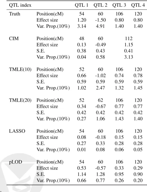
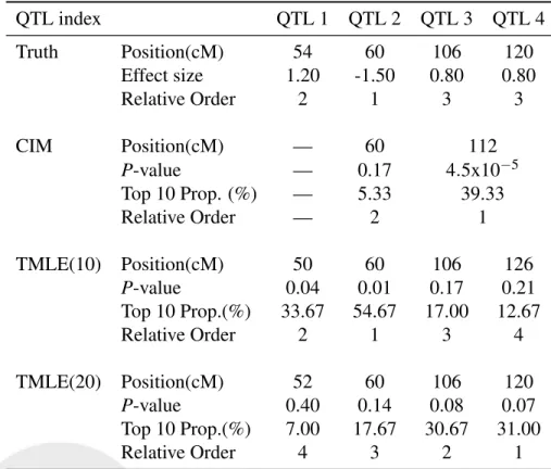
In Figure 1, we present the profiles of effect estimates, p-values, and rankings at each marker for CIM, TMLE(10), and TMLE(20). The true and the estimated main QTL effects are reported in Table 1 along with their p-values, top 10 proportions, and relative orderings. The p-value profiles for CIM, TMLE(10), and TMLE(20) are largely aligned with their effect estimate coun-terparts, although there were slight differences in QTL position estimates, and are reported in Table 2. TMLE(10) has the best performance with respect to separating linked effects. In addi-tion, TMLE(10) has produced the most accurate rankings of the QTL based on QTL p-values. Ranking accuracy was evaluated for a specific marker by the proportion of simulations where that marker’s p-value ranking was less than or equal to 10 among all the markers in a simulation. For TMLE(10), this quantity has mirrored the true effect sizes of the simulated QTL and resulted in a correct relative ordering among the four main QTL effects. CIM missed QTL 1 and merged QTL 3 and QTL 4. The performance of TMLE(20) lies in-between TMLE(10) and CIM. A ranking cutoff of 5 produced similar results.

Table 1: Effect estimates of simulated QTL main effects from CIM, TMLE(10), and TMLE(20). QTL index QTL 1 QTL 2 QTL 3 QTL 4 Truth Position(cM) 54 60 106 120 Effect size 1.20 -1.50 0.80 0.80 Var. Prop.(10%) 3.14 4.91 1.40 1.40 CIM Position(cM) 48 60 112 Effect size 0.13 -0.49 1.15 S.E. 0.38 0.43 0.41 Var. Prop.(10%) 0.04 0.58 3.13 TMLE(10) Position(cM) 52 60 106 120 Effect size 0.66 -1.02 0.74 0.78 S.E. 0.59 0.59 0.59 0.59 Var. Prop.(10%) 1.02 2.47 1.32 1.45 TMLE(20) Position(cM) 52 62 106 120 Effect size 0.34 -0.67 0.77 0.77 S.E. 0.42 0.42 0.42 0.42 Var. Prop.(10%) 0.27 1.06 1.43 1.40 LASSO Position(cM) 54 60 106 120 Effect size 0.08 -0.18 0.15 0.15 S.E. 0.27 0.33 0.28 0.28 Var. Prop.(10%) 0.01 0.08 0.06 0.05 pLOD Position(cM) 54 60 106 120 Effect size 0.53 -0.57 0.33 0.29 S.E. 1.14 1.28 0.95 0.90 Var. Prop.(10%) 0.66 0.77 0.26 0.20

S.E.: standard error.

Var. Prop. (10%): median proportion of explained variance of QTL.

The S.E. of TMLE estimates are averages of the standard error estimates across 300 replicates.

The S.E. of CIM, LASSO, and pLOD estimates are the empirical standard deviations of the effect estimates across 300 replicates.

Table 2:P-values and relative orderings of four simulated QTL main effects from CIM, TMLE(10), and TMLE(20). QTL index QTL 1 QTL 2 QTL 3 QTL 4 Truth Position(cM) 54 60 106 120 Effect size 1.20 -1.50 0.80 0.80 Relative Order 2 1 3 3 CIM Position(cM) — 60 112 P-value — 0.17 4.5x10−5 Top 10 Prop. (%) — 5.33 39.33 Relative Order — 2 1 TMLE(10) Position(cM) 50 60 106 126 P-value 0.04 0.01 0.17 0.21 Top 10 Prop.(%) 33.67 54.67 17.00 12.67 Relative Order 2 1 3 4 TMLE(20) Position(cM) 52 60 106 120 P-value 0.40 0.14 0.08 0.07 Top 10 Prop.(%) 7.00 17.67 30.67 31.00 Relative Order 4 3 2 1

Top 10 Prop.: proportion of the simulations that a QTL is among the top 10 ranked QTL ranked by theirp-values. Effect estimates are averaged over 300 replicates.

The reportedp-values are the medianp-values across 300 replicates.

−1.5 −0.5 0.0 0.5 1.0 1.5 (a) Mean Eff ect Estimate CIM TMLE(10) TMLE(20) 0 1 2 3 4 5 (b) Median P−v

alue (on −log10 scale)

0 50 100 150 200 0.0 0.2 0.4 0.6 0.8 (c) cM T op 10 Propor tion

Figure 1: Estimated main effects of simulated markers and theirp-value and ranking profiles from CIM, TMLE(10), and TMLE(20), plotted against their genomic locations in cM. TMLEs were initalized with CIM. (a) Mean profiles of the estimated main effects at each marker; (b) Median profiles of p-values of estimated main effects, on negative log 10 scale. (c) Proportion of simu-lations that a QTL is ranked top 10 based on their p-values. Triangles represent the locations of simulated main QTL. Arrows or triangles represent the simulated main QTL effects; Stars repre-sent the simulated epistatic effects.

3.2

Additional Analyses

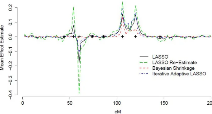
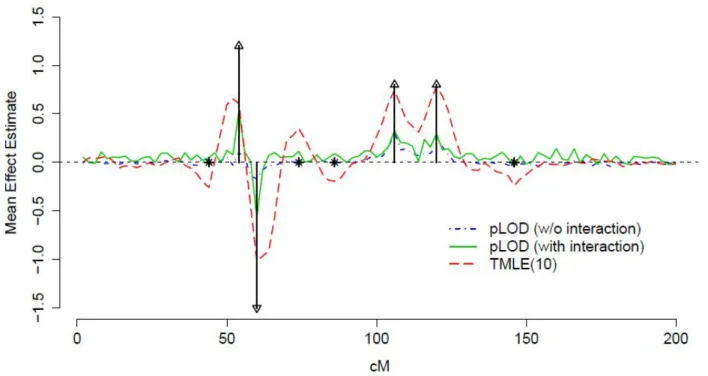
We also analyzed the simulated datasets using a variety of shrinkage methods with main-terms linear models, including the least absolute shrinkage and selection operator (LASSO) (Tibshirani 1996; Friedman et al. 2010), Bayesian shrinkage estimation (H. Wang 2005), iterative adaptive LASSO (W. Sun 2010), and a penalized likelihood approach (pLOD) presented in A. Manichaikul (2009) (Table 1, Figure 2, supplementaryy table S1, and supplementary figure S4). Analyses focused on effect estimates as these methods do not always provide p-value profiles. LASSO de-tected four markers carrying main effects and none of the markers carrying epistatic effects. The effect estimates from LASSO are biased downward. This is expected as LASSO estimator is a shrinkage estimator. We reestimated the effects of each marker detected by LASSO in a multi-variate linear regression. The estimates are moderately improved, on average, and other shrinkage methods produced results similar to LASSO (supplemental figure S2). In addition to the above methods, we used pLOD, allowing pairwise interactions, as pLOD is designed to detect epistatic effects. This led to improved performance compared to a linear model with main effects only, even though the pLOD effect estimates did not outperform TMLE (supplemental figure S3).

Additionally, we examined how the effect estimates of markers associated with epistatsis were affected when ignoring interaction terms in the model by evaluating the marginal effect of the four epistatic markers M_[44], M_[74], M_[86], andM_[146] (supplemental table S2). Estimates from all methods are quite biased, yet TMLE(10) produced overall results closest to the true effects. The performance of TMLE(20) is similar to that of CIM. We also investigated how initial estimators (UR, CIM, and LASSO) affect the performance of TMLE. Results were similar for TMLE(10), but differed for TMLE(20), where CIM provided the best performance (supplemental figure S5 and supplemental table S3). In summary, TMLE produced the most accurate estimates among all investigated methods. A more aggressive marker confounding regression will result in improved bias reduction for a misspecified initial estimator, but also larger variance estimates.

4

Barley Data Analysis

We analyze a barley dataset presented in Hayes et al. (1993), available from

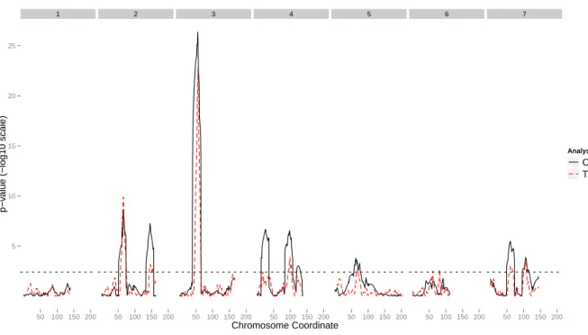
http://www.genenetwork.org/genotypes/SXM.geno and http://wheat.pw.usda.gov/ggpages/SxM /phe-notypes.html. This dataset contains 150 doubled haploid lines derived from the F1 cross of two barley varieties: “Steptoe” and “Morex”. Phenotypes consist of eight agronomic traits measured across multiple environments. Genotypes include 495 markers distributed along barley genome. The purpose of the study is to identify QTL linked to measured agronomic traits. For the ease of demonstration, we only present the analysis of a malting quality trait referred to as “Lodging.” This trait was measured in six enviroments and the average was taken as the phenotype in our analysis. We removed 3 samples and 54 markers that were of low quality (call rate threshold 90%). The genotypes of each marker were coded 1 for Steptoe allele and -1 for Morex allele. Both CIM and TMLE were run to test 1070 positions along the barley genome at an incremental step of 1 centimorgan. CIM was carried out using QTL Cartographer. In TMLE, the initialQ(_n0)was fit to the entire dataset using elastic net, with 50% mixtures ofL1andL2penalties. The marker confounding

mechanismg_n(W)was fit with a linear regression on flanking QTL that are 20cM away from the tested position. In Figure 3, p-value profiles of the analysis are presented (for the profile of effect

0 50 100 150 200 −1.5 −1.0 −0.5 0.0 0.5 1.0 1.5 cM Mean Eff ect Estimate LASSO pLOD TMLE(10)

Figure 2: Mean profiles of estimated main effects of simulated markers from LASSO, pLOD, and TMLE(10), plotted against their genomic locations in cM. TMLEs were initalized with CIM. Arrows represent the simulated main QTL effects; Stars represent the simulated epistatic effects.

Chromosome Coordinate

p−v

alue (−log10 scale)

5 10 15 20 25 1 50 100 150 200 2 50 100 150 200 3 50 100 150 200 4 50 100 150 200 5 50 100 150 200 6 50 100 150 200 7 50 100 150 200 Analysis CIM TMLE

Figure 3: The p-value profile at tested positions for the barley dataset. The x-axis represents cM, and the y-axis is the p-value on negative log 10 scale. The imposed number on top indicates the chromosome number. The black curve represents the result from CIM, and the red curve represents the result from TMLE.

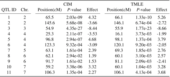
estimates, please see supplemental figure S6), and in Table 3, we report the estimates of all QTL with p-value less than 0.0034 (suggested linkage threshold in Lander and Kruglyak (1995)).

Two major QTL on chromosome 2 (QTL 1) and 3 (QTL 4) are identified by both CIM and TMLE. CIM identified several other QTL as highly significant, while these QTL are borderline significant in TMLE. Typical cases are QTL 2, QTL 4 and QTL 5. This difference is likely due to documented epistatic effects at these sites (Hayes et al. 1993). CIM is a parametric method and its result is sensitive to model misspecification. Our analysis assumed a main effect model that ignores interaction effects, and may lead to biased effect estimates in CIM. In contrast, TMLE is more robust to model misspecification, and hence produces less significant p-values at sites with epistatic effects. TMLE also has a better resolution than CIM, particularly evidenced by the peak on chromosome 5. Our findings are also largely consistent with what was reported previously (Hayes et al. 1993; Zhao and Xu 2012).

We produced an additional simulation study based on this barely dataset to study the classic QTL mapping setting where markers are widely spaced and QTL lie in-between markers with unobserved genotypes (see supplementary materials). This simulation informed several of the analytic choices in the barely data analysis above. This included the finding that due to high and variable correlations among markers, adjusting for markers 10 cM away led to overfitting ingn(W),

and thus was not pursued. We also found two advantages associated with TMLE compared to CIM in this simulation: (1) the resolution of identified QTL from TMLE was better; and (2) TMLE, on average, preserved the correct rankings of simulated QTL while CIM did not (supplemental figure

Table 3: The estimated QTL main effects and positions in cM for the barley dataset.

CIM TMLE

QTL ID Chr. Position(cM) P-value Effect Position(cM) P-value Effect 1 2 65.5 2.03e-09 4.32 66.1 1.33e-10 5.26 2 2 145.6 5.68e-08 -3.66 146.1 6.74e-04 -2.72 3 3 54.9 4.35e-27 -8.44 55.9 1.77e-23 -8.66 4 4 25.3 2.11e-07 -3.53 16.1 3.73e-03 -1.99 5 4 96.8 2.94e-07 4.68 98.1 1.37e-04 3.79 6 4 123.3 9.32e-04 -3.09 120.1 9.20e-03 -2.05 7 5 63.1 1.61e-04 2.39 69.3 1.85e-03 2.76 8 6 62.1 2.94e-02 1.39 60.1 3.10e-03 2.57 9 6 91.7 1.61e-02 1.53 81.1 2.09e-03 -2.41 10 7 59.2 3.38e-06 3.32 60.1 1.04e-03 3.28 11 7 106.3 1.35e-04 2.27 106.1 4.13e-04 3.68 S7b-c).

5

Discussion

Targeted maximum likelihood learning is a novel flexible semiparametric methodology with broad applications in QTL mapping. Analysis of variance, univariate regression, various forms of interval mapping, and machine learning techniques have been proposed and implemented for QTL map-ping. However, current practice relies heavily on parametric models. While parametric methods offer inference viap-values, bias is a substantial issue. Machine learning algorithms offer flexibil-ity, yet lack inference and are designed for prediction over effect estimation. TMLE allows both effective inference and bias reduction, as well as the incorporation of machine learning without substantial computational burden.

In this paper, we explored TMLE in QTL mapping with simulations and a data analysis. We compared TMLE with popular approaches, such as UR, CIM, and shrinkage methods. In our simulations, these methods were substantially more biased than TMLEs, and TMLEs improved on their estimates and had the most accurate rankings of QTL. TMLE and CIM were also compared in a barley data set, with TMLE displaying less noise. In the analysis of the barley data set, we initialized TMLE with elastic nets, demonstrating its ability to incorporate machine learning algorithms.

In summary, a targeted learning approach for QTL mapping has multiple advantages. Firstly, semiparametric models place fewer unrealistic restrictions on the functional form of the data. Sec-ondly, precision of the QTL mapping is improved in the bias-reduction step. Thirdly, machine learning algorithms, such as random forests or more aggressive ensembling techniques (van der Laan et al. 2007; van der Laan and Rose 2011), can be incorporated into the prediction steps to allow for more flexible estimation. Lastly,p-values are available to generate ranked lists of QTL.

6

Acknowledgement

We want to thank Dr. Shizhong Xu for his generosity to provide us a clean and compiled version of the barley dataset.

References

S. Sen B.S. Yandell K.W. Broman A. Manichaikul, J.Y. Moon. A model selection approach for the identification of quantitative trait loci in experimental crosses, allowing epistasis. Genetics, 181:1077–1086, 2009.

C.J. Basten, B.S. Weir, and Z.B. Zeng. QTL Cartographer, 2001. URL

http://statgen.ncsu.edu/qtlcart/.

L. Breiman. Random forests. Mach Learn, 45:5–32, 2001.

J. Friedman, T. Hastie, and R. Tibshirani. Regularization paths for generalized linear models via coordinate descent. Journal of Statistical Software, pages 1–22, 2010.

S. Gruber and M.J. van der Laan. An application of collaborative targeted maximum likelihood estimation in causal inference and genomics. Int J Biostat, 6(1), 2010a.

S. Gruber and M.J. van der Laan. A targeted maximum likelihood estimator of a causal effect on a bounded continuous outcome. Int J Biostat, 6(1):Article 26, 2010b.

X. Li G.L. Masinde S. Mohan D.J. Baylink S. Xu H. Wang, Y.M. Zhang. Bayesian shrinkage estimation of quantitative trait loci parameters. genetics. Genetics, 170:465–480, 2005.

C.S. Haley and S.A. Knott. A simple regression method for mapping quantitative trait loci in line crosses using flanking markers. Heredity, 1992.

P. M. Hayes, B. H. Liu, S. J. Knapp, F. Chen, B. Jones, T. Blake, J. Franckowiak, D. Rasmusson, M. Sorrells, S. E. Ullrich, D. Wesenberg, and A. Kleinhofs. Quantitative trait locus effects and environmental interaction in a sample of north american barley germ plasm. Theor Appl Genet, 87:392–401, 1993.

S.C. Heath. Markov chain Monte Carlo segregation and linkage analysis of oligogenic models.

Am J Hum Genet, 1997.

R.C. Jansen. Interval mapping of multiple quantitative trait loci. Genetics, 1993.

C.H. Kao, Z.B. Zeng, and R.D. Teasdale. Multiple interval mapping for quantitative trait loci.

Genetics, 1999.

E. Lander and L. Kruglyak. Genetic dissection of complex traits: guidelines for interpreting and reporting linkage results. Nat Genet, 11:241–247, 1995.

E.S. Lander and D. Botstein. Mapping Mendelian factors underlying quantitative traits using RFLP linkage maps. Genetics, 1989.

S.S.F. Lee, L. Sun, R. Kustra, and S.B. Bull. EM-random forest and new measures of variable importance for multi-locus quantitative trait linkage analysis. Bioinformatics, 2008.

S. Rose and M.J. van der Laan. Simple optimal weighting of cases and controls in case-control studies. Int J Biostat, 4(1):Article 19, 2008.

J.M. Satagopan, B.S. Yandell, M.A. Newton, and T.C. Osborn. A Bayesian approach to detect quantitative trait loci using Markov chain Monte Carlo. Genetics, 1996.

K. Sax. The association of size difference with seed-coat pattern and pigmentation inPhaseolus vulgaris. Genetics, 1923.

M.J. Sillanpaa and E. Arjas. Bayesian mapping of multiple quantitative trait loci from incomplete inbred line cross data. Genetics, 1998.

O.M. Stitelman and M.J. van der Laan. Collaborative targeted maximum likelihood for time-to-event data. Int J Biostat, 6(1):Article 21, 2010.

J.M. Thoday. Location of polygenes. Nature, 1960.

R. Tibshirani. Regression shrinkage and selection via the lasso. J. Royal. Statist. Soc B., 58: 267–288, 1996.

C. Tuglus and M.J. van der Laan. Targeted methods for biomarker discovery. In M.J. van der Laan and S. Rose, Targeted Learning: Causal Inference for Observational and Experimental Data. Springer, Berlin Heidelberg New York, 2011.

M.J. van der Laan and S. Rose. Targeted Learning: Causal Inference for Observational and

Experimental Data. Springer, Berlin Heidelberg New York, 2011.

M.J. van der Laan and Daniel B. Rubin. Targeted maximum likelihood learning. Int J Biostat, 2 (1):Article 11, 2006.

M.J. van der Laan, E.C. Polley, and A.E. Hubbard. Super learner. Stat Appl Genet Mol, 6(1): Article 25, 2007.

F. Zou W. Sun, J.G. Ibrahim. Genome-wide multiple loci mapping in experimental crosses by the iterative adaptive penalized regression. Genetics, 185:349–359, 2010.

H. Wang, S. Rose, and M.J. van der Laan. Finding quantitative trait loci genes with collaborative targeted maximum likelihood learning. Stat Prob Lett, 81(7):792–796, 2011.

Z.B. Zeng. Precision mapping of quantitative trait loci. Genetics, 1994.

F. Zhao and S. Xu. An expectation and maximization algorithm for estimating q x e interaction effects. Theor Appl Genet, 124:1375–1387, 2012.

Simulation Study

We additionally compared the results of TMLE(10) and TMLE(20) using three different initial estimators: univariate regression, CIM, and LASSO. The results of these three methods were improved upon the 2nd stage correction, and differences among them were reduced. The extent

of improvement depends on which gn(W) was used. For TMLE(10), the final results are almost

identical for all three initial estimators including univariate regression despite of its inferior performance. The univariate regression has the largest variance estimates. For TMLE(20), we do see performance differences for these three methods, with CIM providing the best results and univariate regression the worst (supplemental figure S7 and supplemental table S3). This

demonstrates the double robustness and local efficiency of TMLE: a g_n(W) with more

predictive power can better compensate a suboptimal Qn

(0)_{, and a better}

Qn

(0) _{produces estimates}

of smaller variances.

It is worth noting that when UR is used as Qn

(0)_{, TMLE is mathematically equivalent to a simple}

regression Y ~A+W₁+W₂. This is because we have used very simple models for Qn

(0)_and

gn(W), and hence reduced our semiparametric model to a parametric one. In this case, the

success of TMLE completely relies on correct specification of W1 and W2.

Supplemental Simulation

This supplemental simulation reproduces the classic QTL mapping setting where markers are widely spaced and QTL lie in-between markers with unobserved genotypes. We used the data structure in a doubled haploid barley dataset analyzed in the latter part of the main paper (Section 4). Samples and markers with greater than 10% missing rate were excluded from simulation, resulting in 147 samples and 441 markers on 7 chromosomes. We selected 10 markers among the 441 markers and simulated phenotypic values using these markers with a linear main-term model. The selected markers were then deleted from the simulated dataset to create the unobserved QTL. The effect size of simulated QTL ranges from 0.14 to 0.35, explaining 1.28% to 7.97% of the total variance. The distance from a QTL to a marker ranges from 0.6 cM to 15.7 cM. The error term was drawn from a normal distribution with mean 0 and standard deviation 1. Details of positions and effect sizes of simulated QTL can be found in supplemental table S4. The simulation was replicated 100 times.

We tested 1070 positions at an incremental distance of 1 cM along the genome in each simulated replicate with CIM and TMLE. The genotypes of putative QTL at tested positions were imputed

with the Haley-Knott regression. The initial estimator Qn

(0) _{in TMLE was fit with an elastic net}

we analyzed the real data (Section 4). Due to high and variable correlations among markers in

this dataset, adjusting markers 10 cM away led to overfitting in g_n(W) and was not pursued. The

g_n(W) was fitted with a linear regression on neighboring markers no less than 20 cM away from

the tested position, resulting in a Pearson's correlation coefficient of 0.7 on average between the tested position and adjusted markers. Supplemental figure S7 presents the profiles of the

estimated effect sizes, p-values, and ranking proportions from CIM and TMLE. Ranking

proportion is defined as the proportion of simulations that a QTL is ranked top 10 based on their

p-values.

TMLE identified simulated QTL in a comparable way as CIM, demonstrating its utility for classic QTL mapping. Two advantages are associated with TMLE compared to CIM: (1) the resolution of identified QTL from TMLE is better; and (2) TMLE on average preserves the correct rankings of simulated QTL (supplemental figure S7b-c) while CIM did not (5 QTL with small effect sizes were missed among the top 10 ranked QTL, and the ranks of QTL 1 on chromosome 2 and QTL 5 on chromosome 4 were over-estimated) (supplemental figure S7c).

The p-values from TMLE are more conservative than those from CIM. However, as mentioned

before, this “conservativeness” may in fact be a more honest evaluation of the significance of a QTL. Numeric details of the results such as standard errors and QTL rankings can be found in supplemental table S4. We also reported the effect estimates and rankings from the elastic net in supplemental figure S8 for interested readers to compare results pre and post adjustment of

TABLE S1

The mean effect sizes of simulated main QTL estimated from various algorithms.

Main QTL QTL1 QTL2 QTL3 QTL4 Position (cM) 54 60 106 120 True Effect 1.2 -1.5 0.8 0.8 UR 0.23 (0.26) 0.01 (0.26) 1.05 (0.26) 1.07 (0.26) CIM -0.05 (0.40) -0.49 (0.43) 0.97 (0.54) 0.92 (0.58) LASSO 0.08 (0.27) -0.18 (0.33) 0.15 (0.28) 0.15 (0.28) IAL 0.03 (0.22) -0.11 (0.33) 0.19 (0.48) 0.17 (0.42) Bayesian Shrinkage 0.00 (0.02) -0.01 (0.02) 0.14 (0.17) 0.05 (0.12) LASSO Re-Estimate 0.21 (0.64) -0.39 (0.67) 0.24 (0.47) 0.21 (0.37) pLOD Epistatic Model 0.53 (1.14) -0.57 (1.28) 0.33 (0.95) 0.29 (0.90) pLOD Main Effect Model 0.10 (0.24) -0.17 (0.42) 0.31 (0.71) 0.16 (0.48) TMLE (10) 0.61 (0.66) -1.02 (0.58) 0.74 (0.62) 0.78 (0.58) TMLE (20) 0.10 (0.58) -0.65 (0.55) 0.77 (0.68) 0.77 (0.60)

Numbers in brackets are standard errors. TMLE used CIM as the initial estimator. Standard errors for TMLE were calculated as the mean of estimated standard errors from TMLE, and standard errors for other methods were calculated as the standard deviation of effect sizes across 300 replicates.

TABLE S2

The mean effect sizes of the marginal effect of simulated epistatic QTL estimated from various algorithms.

Epistatic QTL Position (cM) 44 74 86 146 True Effect -0.5 0.7 -0.4 -0.6 UR 0.11 (0.27) 0.37 (0.26) 0.54 (0.25) 0.46 (0.27) CIM 0.03 (0.35) 0.03 (0.41) -0.07 (0.37) -0.19 (0.35) LASSO 0.00 (0.07) 0.01 (0.12) 0.00 (0.08) -0.01 (0.10) IAL 0.00 (0.09) 0.01 (0.13) 0.00 (0.06) 0.00 (0.05) Bayesian Shrinkage 0.00 (0.00) 0.00 (0.01) 0.00 (0.01) 0.00 (0.00) LASSO Re-Estimate -0.02 (0.24) 0.03 (0.23) -0.01 (0.20) -0.03 (0.27) PLOD Epistatic Model 0.05 (0.89) 0.11 (0.93) 0.09 (0.90) -0.05 (0.56) pLOD Main Effect Model 0.02 (0.11) 0.00 (0.06) 0.01 (0.10) -0.02 (0.11)

TMLE (10) -0.26 (0.57) 0.35 (0.57) -0.19 (0.57) -0.24 (0.57) TMLE (20) 0.03 (0.41) -0.01 (0.42) -0.10 (0.41) -0.23 (0.41)

Effect sizes were averaged over 300 replicates. Numbers in brackets are standard errors. TMLE used CIM as the initial estimator. Standard errors for TMLE were calculated as the mean of estimated standard errors from TMLE, and standard errors for other methods were calculated as the standard deviation of effect sizes across 300 replicates.

TABLE S3

The simulated QTL main effects and their mean TMLE estimates with different initial estimators.

Main Effect QTL

QTL1 QTL2 QTL3 QTL4

Truth Position (cM) 54 60 106 120

Effect 1.2 -1.5 0.8 0.8

TMLE Estimates Initial Estimator TMLE(10) UR 0.61 (0.60) -1.03 (0.60) 0.75 (0.59) 0.82 (0.59) CIM 0.61 (0.58) -1.02 (0.58) 0.74 (0.58) 0.78 (0.58) LASSO 0.60 (0.58) -1.03 (0.58) 0.75 (0.58) 0.80 (0.58) TMLE(20) UR 0.03 (0.43) -0.63 (0.43) 1.01 (0.43) 1.02 (0.42) CIM 0.10 (0.42) -0.65 (0.42) 0.77 (0.42) 0.77 (0.42) LASSO 0.05 (0.42) -0.64 (0.42) 0.90 (0.42) 0.91 (0.42)

Effect sizes were averaged over 300 replicates. Numbers in brackets are standard errors. Standard errors for TMLE were calculated as the mean of estimated standard errors from TMLE, and standard errors for other methods were calculated as the standard deviation of effect sizes across 300 replicates.

TABLE S4

The simulated QTL main effects from barley data set and their summary metrics of estimates from various algorithms.

QTL Index Marker QTL 1 QTL 2 QTL 3 QTL 4 QTL 5 QTL 6 QTL 7 QTL 8 QTL 9 QTL 10 Truth Chromosome 2 2 3 4 4 4 5 6 6 7 Position (cM) 65.5 90.2 55.1 16.1 98.5 120.3 69.3 62.1 91.7 60.2 Marker Before (cM) 2.2 7.1 0.7 0.8 2.7 2.2 2.1 1.4 4.4 2 Marker After (cM) 0.8 1.4 0.6 3.7 1.4 15.7 1.5 3.2 2.9 4.1 Effect Size 0.28 0.31 0.35 0.18 0.25 0.22 0.2 0.17 0.15 0.14 Var. Prop. (%) 4.97 5.96 7.97 2.03 3.94 3.1 2.56 1.88 1.47 1.28 Relative Order 3 2 1 7 4 5 6 8 9 10 CIM Position (cM) 69.1 91.1 56.9 13.1 102.1 126.1 71.3 62.1 85.1 56.1 Effect Size 0.4191 0.2173 0.3437 0.1698 0.3492 0.2013 0.1615 0.1819 0.2196 0.1425 S.E. 0.0928 0.1411 0.0824 0.0873 0.0944 0.1226 0.0884 0.1098 0.0854 0.0789

P-value 1.10E-05 6.88E-02 6.39E-05 7.05E-02 1.03E-04 7.56E-02 4.86E-02 5.67E-02 9.93E-03 9.79E-02

Var. Prop. (%) 8.55 1.28 6.64 1.42 6.59 1.29 1.47 1.42 2.73 1.11

Top 10 Prop. (%) 47 1 17 0 20 0 0 0 1 0

Relative Order 1 7 2 8 3 9 5 6 4 10

Elastic Net Position (cM) 67.1 91.1 55.9 14.1 100.1 118.1 72.3 61.1 96.1 58.1

Effect Size 0.0387 0.0166 0.0412 0.0154 0.0280 0.0105 0.0169 0.0137 0.0126 0.0139 S.E. 0.0607 0.0359 0.0539 0.0369 0.0433 0.0261 0.0342 0.0324 0.0286 0.0319 Var. Prop. (%) 0 0 0.02 0 0 0 0 0 0 0 Top 10 Prop. (%) 24 11 29 8 22 4 9 10 8 8 Relative Order 2 5 1 6 3 10 4 8 9 7 TMLE(20) Position (cM) 65.1 95.1 55.9 18.1 100.1 117.1 72.3 62.1 96.1 57.1 Effect Size 0.2719 0.1634 0.3303 0.1577 0.1921 0.1792 0.1678 0.1564 0.12 0.1124 S.E. 0.1097 0.1180 0.1019 0.0968 0.1185 0.0996 0.1232 0.1060 0.0905 0.1305 P-value 0.0104 0.1412 0.0010 0.1029 0.1013 0.0787 0.1406 0.1304 0.1828 0.3457 Var. Prop. (%) 4.18 1.45 6.27 1.16 1.58 1.8 1.87 1.21 0.86 0.82 Top 10 Prop. (%) 16 5 32 4 4 10 1 4 3 2 Relative Order 2 8 1 5 4 3 7 6 9 10

Marker Before/After: the nearest markers (before imputation) to the 5’- and 3’-end of each simulated QTL; S.E.: standard error; Var. Prop.: median proportion of explained variance of QTL; Top 10 Prop.: proportion of the simulations that a QTL is among the top 10 ranked QTL, ranked by their p-values for CIM and TMLE and by their effect sizes for Elastic Net. Position estimates took the location of the top marker, within the 20cM window (10cM each side) of each simulated QTL, identified in the median p-value profiles for CIM and TMLE and in the mean estimated effect profile for CIM. Effect estimates are averaged over 100 replicates. The S.E. of TMLE estimates are averages of the standard error estimates across 100 replicates. The S.E. of CIM and Elastic Net estimates are the empirical standard deviations of the effect estimates across 100 replicates. The reported p-values are the median p-p-values across 100 replicates. Relative order of the simulated QTL is ranked by effect size for the truth and Elastic Net and by p-value for CIM and TMLE.

FIGURE S1. — Estimated main effects of simulated markers and their p-values from UR, TMLE(10), and TMLE(20), plotted against their genomic locations in cM. TMLEs were initialized with UR. (a) Mean profiles of the estimated main effects at each marker; (b) Median profiles of p-values of estimated main effects, on negative log 10 scale. Arrows or triangles represent the simulated main QTL effects; Stars represent the simulated epistatic effects.

0 50 100 150 200 -1 .5 -1 .0 -0 .5 0. 0 0. 5 1. 0 1. 5 (a) cM M ea n Ef fe ct E st im at e UR TMLE(10) TMLE(20) 0 50 100 150 200 0 1 2 3 4 5 (b) cM M ed ia n P-va lu e (o n -lo g1 0 sca le ) UR TMLE(10) TMLE(20)

FIGURE S2. — Estimated main effects of simulated markers using LASSO, re-estimated LASSO, Bayesian Shrinkage method, and Iterative Adaptive LASSO (IAL). The effect estimates are plotted against their genomic locations in cM. The plus sign (+) indicates locations of QTL with main effect, and star sign (*) indicates locations of QTL carrying epistatic effects.

FIGURE S3. — Estimated main effects of simulated markers using a penalized LOD (pLOD) approach. The effect estimates are plotted against their genomic locations in cM. Two models were used in the pLOD procedure. One model has main terms only allowing no interactions, and the other model allows for both main terms and pairwise interactions. The arrows indicate true locations and effects of QTL with main effect, and star sign (*) indicates locations of QTL carrying epistatic effects.

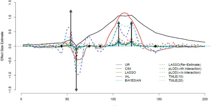
FIGURE S4. — Estimated main effects of simulated markers using various algorithms and methods. UR: univariate regression; IAL: iterative adaptive LASSO; BAYESIAN: Bayesian shrinkage method; The effect estimates are plotted against their genomic locations in cM. The arrows indicate true locations and effects of QTL with main effect, and star sign (*) indicates locations of QTL carrying epistatic effects.

FIGURE S5.—Mean profiles of the main effects of simulated markers estimated from TMLE(10) and TMLE(20) using univariate regression (UR), CIM, and LASSO as initial estimators. The effect sizes are plotted against their genomic locations in cM. Arrows represent the simulated main QTL effects; Stars represent the simulated epistatic effects.

cM Estimate −1.5 −1.0 −0.5 0.0 0.5 1.0 TMLE10 * * * * 50 100 150 200 TMLE20 * * * * 50 100 150 200 InitialEstimator UR CIM LASSO

FIGURE S6. —The profile of effect estimates at tested positions for the barley dataset. The x-axis is the genome position in cM; the y-axis is the p-value on negative log 10 scale. The imposed number on top indicates the chromosome number. Blue curve represents CIM, and red curve represents TMLE.

Chromosome Coordinate Ef fe ct Es tim a te -8 -6 -4 -2 0 2 4 1 50 100 150 200 2 50 100 150 200 3 50 100 150 200 4 50 100 150 200 5 50 100 150 200 6 50 100 150 200 7 50 100 150 200 Analysis CIM TMLE

FIGURE S7.—Estimated main effects of simulated markers based on the barely dataset and their p-values and ranking profiles from CIM and TMLE, plotted against their genomic locations in cM. (a) Mean profiles of the estimated main effects; (b) Median profiles of p-values of estimated main effects, on negative log 10 scale; (c) Proportion of simulations that a QTL is ranked top 10 based on their p-values. Arrows represent the simulated main QTL effects. Triangles represent the locations of simulated main QTL. 1 2 3 4 5 6 7 −0.1 0.0 0.1 0.2 0.3 0.4 0 50 100 150 200 0 50 100 150 200 0 50 100 150 200 0 50 100 150 200 0 50 100 150 200 0 50 100 150 200 0 50 100 150 200 Chromosome Coordinate Mean Eff ect Estimate Analysis CIM TMLE (a) Effect Size

FIGURE S8. — Estimated main effects of simulated markers and their ranking profiles from Elastic Net, plotted against their genomic locations in cM. (a) Mean profiles of the estimated main effects; (b) Proportion of simulations that a QTL is ranked top 10 based on their estimated main effects. Triangles represent the locations of simulated main QTL.