Evolutionary neural architecture search for deep learning

(1)

Copyright by

Jason Zhi Liang 2018

(2)

The Dissertation Committee for Jason Zhi Liang

certifies that this is the approved version of the following dissertation:

Evolutionary Neural Architecture Search for Deep

Learning

Committee:

Risto Miikkulainen, Supervisor Ross Baldick

Qixing Huang Peter Stone

(3)

Evolutionary Neural Architecture Search for Deep

Learning

by

Jason Zhi Liang,

DISSERTATION

Presented to the Faculty of the Graduate School of The University of Texas at Austin

in Partial Fulfillment of the Requirements

for the Degree of

DOCTOR OF PHILOSOPHY

THE UNIVERSITY OF TEXAS AT AUSTIN December 2018

(4)

This thesis is dedicated to my parents, who have supported my dreams of pursuing a doctorate degree, and to all the UTCS PhD students that are

(5)

Acknowledgments

I wish to thank my research supervisor Risto Miikkulainen for his in-valuable advice and feedback that helped guide my research over the past few years. It was due to Risto’s graduate course that I was introduced to neural networks and evolutionary computation in the first place. Without his guid-ance, my dreams of becoming an artificial intelligence research scientist would not have been possible.

I will also like to acknowledge everyone in the Neural Network Research Group at UT Austin, especially Elliot Meyerson, for their helpful contributions and suggestions to help me further my research. Elliot collaborated with me on several projects and experiments and proved to be a very inspiring and thought provoking colleague. I would also give thanks to the LEAF team at Sentient Technologies, especially Dan Fink and Karl Mutch, for their assis-tance in building the infrastructure and framework needed for my research. Lastly, I like to thank my committee members, Peter Stone, Ross Baldick, and Qixing Huang, for their thoughtful suggestions and patience in reviewing my dissertation.

(6)

Evolutionary Neural Architecture Search for Deep

Learning

Publication No.

Jason Zhi Liang, Ph.D.

The University of Texas at Austin, 2018 Supervisor: Risto Miikkulainen

Deep neural networks (DNNs) have produced state-of-the-art results in many benchmarks and problem domains. However, the success of DNNs depends on the proper configuration of its architecture and hyperparameters. DNNs are often not used to their full potential because it is difficult to deter-mine what architectures and hyperparameters should be used. While several approaches have been proposed, computational complexity of searching large design spaces makes them impractical for large modern DNNs.

This dissertation introduces an efficient evolutionary algorithm (EA) for simultaneous optimization of DNN architecture and hyperparameters. It builds upon extensive past research of evolutionary optimization of neural net-work structure. Various improvements to the core algorithm are introduced, including: (1) discovering DNN architectures of arbitrary complexity; (1) gen-erating modular, repetitive modules commonly seen in state-of-the-art DNNs;

(7)

(3) extending to the multitask learning and multiobjective optimization do-mains; (4) maximizing performance and reducing wasted computation through asynchronous evaluations. Experimental results in image classification, image captioning, and multialphabet character recognition show that the approach is able to evolve networks that are competitive with or even exceed hand-designed networks. Thus, the method enables an automated and streamlined process to optimize DNN architectures for a given problem and can be widely applied to solve harder tasks.

(8)

List of Tables

3.1 Node and global hyperparameters evolved in the CIFAR-10 do-main. They show just how large of a search space that Deep-NEAT is exploring. . . 44 4.1 Summary of classification accuracy of best evolved networks

from different approaches on CIFAR-10 domain. The networks evolved using DeepNEAT and CoDeepNEAT are highlighted in bold. The networks produced through architecture or hyper-parameter search are labeled with an asterisk. Both CoDeep-NEAT and DNGO outperform the manually designed Network-in-Network. . . 58 4.2 Node and global hyperparameters evolved for the image

cap-tioning case study. They show the size of the search space ex-plored by CoDeepNEAT. . . 62 4.3 Summary of performance of different approaches on MSCOCO

domain. The networks produced through architecture or hyper-parameter search are labeled with an asterisk. The evolved net-work using CoDeepNEAT (highlighted in bold) improves over the hand-designed baselines and other architecture search meth-ods. In particular, it was able to beat the Show and Tell network network by 5%. . . 66 5.1 Average validation and test accuracy over 20 tasks for each

algorithm. CMSR performs the best as it combines both module and routing evolution. Pairwise t-tests show all differences are statistically significant with p <0.05. . . 93 5.2 Summary of different search spaces; for normal and expanded,

the input size is 224×224. For encoder, the input size is 28×28. 100 5.3 AUROC on test set for existing approaches that use

hand-designed architectures and networks which are evolved using CMSR. CMSR combined with the hypercolumn approach re-sults in an architecture that is competitive with the state-of-the-art. . . 103

(13)

List of Figures

2.1 A visualization of a number of DNN architectures that been explored so far by the deep learning research community [148]. This diversity suggests that architecture choice is important. . 15 2.2 Figure 2.2a shows how NEAT [141] mutates a chromosome

(rep-resenting a neural network) by either incrementally adding a node (neuron) or a edge (weight) between two nodes. Fig-ure 2.2b shows how two chromosomes perform crossover by swapping edges whose innovation numbers match. NEAT can be extended to neural architecture search by representing layers in a DNN as nodes. . . 19 2.3 A visualization of a set of solutions with respect to two

ob-jectives (network complexity and fitness) and the Pareto front (green line) where the Pareto optimal solutions reside. The Pareto front contain the best possible trade-offs between the two objectives. . . 25 3.1 Overview of the algorithm for DeepNEAT and how it evolves

networks. The main difference between NEAT and DeepNEAT is that in DeepNEAT the chromosome represents DNN archi-tectures at the layer level rather than at the neuron level. . . . 37 3.2 Figure 3.2a shows an example DeepNEAT chromosome while

Figure 3.2b shows corresponding DNN architecture that is cre-ated from parsing the chromosome. Note the chromosome graph is represented as a list of nodes and edges and each node has its own set of evolvable hyperparameters. The chromosome also has a set of global hyperparameters that are relevant to the DNN as a whole. This representation allows the evolution of arbitrary DNN topologies. . . 38 3.3 Examples of the images from the 10 classes of CIFAR-10 dataset

[73]. As a standard benchmark for testing DNNs, this dataset is a good way to evaluate the effectiveness of neural architectures discovered by DeepNEAT. . . 43 3.4 Visualization of the best network evolved by DeepNEAT on the

CIFAR-10 domain. This architecture includes a lot of short-cut connections that lack of any regular, modular structure. The performance of this architecture is comparable to a similar hand-designed network [87]. . . 45

(14)

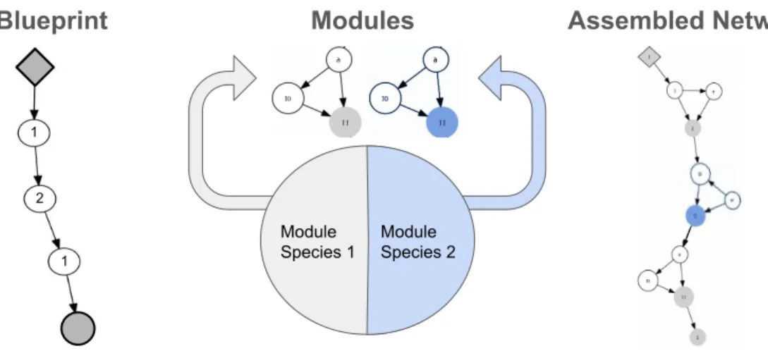
4.1 GoogLeNet [145], an example of a DNN with modular and repetitive structure. The inception module is shown on the left while the full network architecture is shown on the right (with the module circled in red). . . 48 4.2 A visualization of how CoDeepNEAT assembles networks for

fit-ness evaluation. Modules and blueprints are assembled together into a network through replacement of blueprint nodes with cor-responding modules. This approach allows evolving repetitive and deep structures seen in many recent DNNs. . . 50 4.3 Overview of the algorithm for CoDeepNEAT and how it uses

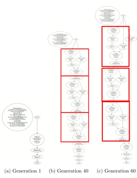
co-evolution to create assembled networks from separate blueprint and module populations. . . 51 4.4 Visualization of best assembled networks discovered by

CoDeep-NEAT at generations 1, 40, and 60. In the first generation, the networks are minimal and have no modules. However, by gen-eration 40, the networks contain modules that are repeated at multiple locations (highlighted in red). . . 52 4.5 Overview of the GAES, a generic version of CoDeepNEAT-AES

that can be applied to any parallel but synchronous EA. . . . 55 4.6 Overview of CoDeepNEAT-AES, an asynchronous extension of

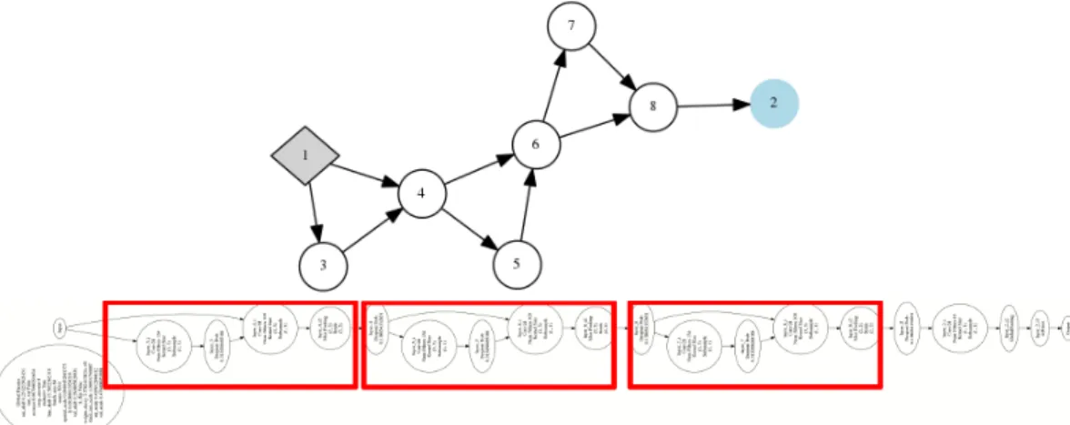
CoDeepNEAT that can take full advantage of a pool of workers for evaluations, made available through the completion service. 56 4.7 Top: High level visualization of the best network evolved by

CoDeepNEAT for the CIFAR-10 domain. Node 1 is the in-put layer, while Node 2 is the outin-put layer. The network has repetitive structure because its blueprint reuses same module in multiple places. Bottom: A more detailed visualization of the entire network with the locations of the modules highlighted in red. The use of modules allowed CoDeepNEAT to beat both DeepNEAT and a hand-designed architecture. . . 60 4.8 Some examples of the types of images in the MSCOCO dataset:

(a) iconic object images, (b) iconic scene images, and (c) non-iconic images [22]. . . 61 4.9 Visualization of the best architecture found by evolution. Among

the components in its unique structure are six LSTM layers, four summing merge layers, and several skip connections. A single module architecture (highlighted in red) consisting of two LSTM layers merged by a sum is repeated three times. There is a path from the input through dense layers to the output that bypasses all LSTM layers, providing the softmax with a more direct view of the current input. The power of the architecture seems to come from the many shortcut connections, which are unlikely to have been discovered by hand. . . 65

(15)

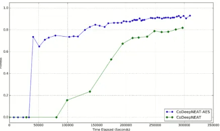
4.10 A plot of fitness versus time elapsed for synchronous CoDeep-NEAT and CoDeepCoDeep-NEAT-AES. Each marker in the plot repre-sents the fitness at a different generation. At any given time, CoDeepNEAT-AES was able to achieve much better fitness. . 68 4.11 A plot of fitness versus number of generations elapsed for

syn-chronous CoDeepNEAT and CoDeepNEAT-AES. This result shows that both algorithms achieved the same fitness when com-pared by generations. However, the generations for CoDeepNEAT-AES were much shorter in duration. . . 68 4.12 A comparison of CoDeepNEAT against the networks discovered

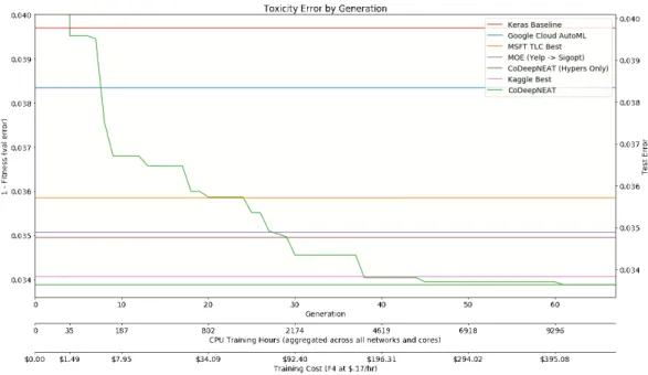
via several commercially available methods, including Kaggle, MSFT TLC, MOE, and Google AutoML. The Y-axis shows best fitness/accuracy achieved so far, while the X-axis shows the generations, total training time, and total amount of money spent on cloud compute. As the plot shows, CoDeepNEAT is gradually able to discover better networks, eventually finding one in the 40th generation that beats all other approaches. . . 72 4.13 A visualization of the best network discovered by CoDeepNEAT

in the Wikidetox domain. As the network architecture shows, it is most optimal to use a combination of both simple and complex modules within the blueprint of the network. . . 74 4.14 An iconic image from an online magazine captioned by an evolved

model. The model provides a suitably detailed description with-out any unnecessary context. . . 77 4.15 Results for captions generated by an evolved model for the

online magazine images rated from 1 to 4, with 4=Correct, 3=Mostly Correct, 2=Mostly Incorrect, 1=Incorrect. Left: On iconic images, the model is able to get about one half correct; Right: On all images, the model gets about one fifth correct. The superior performance on iconic images shows that it is use-ful to build supplementary training sets for specific image types. 78 4.16 Top: Four good captions. The model is able to abstract about

ambiguous images and even describe drawings, along with pho-tos of objects in context. Bottom: Four bad captions. When it fails, the output of the model still contains some correct sense of the image. The results overall are promising and suggest that the model can be improved by including more difficult images in the training set. . . 79 5.1 The relationships of various MTL architectures described in this

chapter. The soft-ordering method [99] is used as the start-ing point, extendstart-ing it with CoDeepNEAT, leadstart-ing to CM and CMSR on the bottom. . . 83

(16)

5.2 Example soft-ordering network with three shared layers [99]. Soft-ordering learns how to use the same layers in different lo-cations by learning a tensor S of task-specific scaling parame-ters. S is learned jointly with the Wd, to allow flexible sharing across tasks and depths. This architecture enables the learning of layers that are used in different ways at different depths for different tasks. . . 85 5.3 High-level algorithm outlines of CM and CMSR, illustrating

how they are similar and different from each other. In partic-ular, the algorithms differ in whether or not the blueprint is evolved along with the modules (see line 7 in Algorithm 6). . . 86 5.4 Comparison of fitness (validation accuracy after partial training

for 3000 iterations) over generations of single runs of CM and CMSR. Solid lines show the fitness of best assembled network and dotted line show the mean fitness. Both methods reach a similar fitness, but CMSR is slower to converge. . . 94 5.5 Comparison of fitness over generations of CM with disabling,

enabling, and evolving module weight sharing. No sharing is better than forced sharing, but evolvable sharing outperforms them both, validating the approach. . . 95 5.6 Visualizations of the best networks evolved by CM (Figures 5.6a

and 5.6b) and CMSR (Figures 5.6c and 5.6d) on the Omniglot domain. The module routing for CM is fixed but is evolvable in CMSR. The module routing (blueprint) evolved by CMSR contains many shortcut connections and could be a possible factor in CMSR’s superior performance. Both methods evolve a mixture of both complex and simple module architectures. . 97 5.7 The top row shows negative examples of images from the Chest

X-ray dataset where no disease is present. The bottom row show positive examples where the images do show a disease. . 98 5.8 Comparison of fitness over generations of CMSR with different

search spaces as described in Table 5.2. Solid lines show the fit-ness of best assembled network and dotted lines shows the mean fitness. The hypercolumn search space is quickest to converge and reaches the best fitness. . . 102 5.9 Overview of the best architectures evolved for the expanded

(Figures 5.9a and 5.9b) and hypercolumn (Figures 5.9c and 5.9d) search spaces. The best hypercolumn network is signifi-cantly simpler than the best expanded network. . . 105 6.1 Overview of lower and upper levels of MCDN perform ranking

of individuals and also how the Pareto front is calculated from two objectives. . . 111

(17)

6.2 List of the hand-crafted features used to characterize the be-havior of each evolved network for novelty search. The novelty score generated using the behavior metric is used as a secondary objective along with fitness. . . 113 6.3 Comparison of fitness over generations of MCDN

(multiobjec-tive) and CoDeepNEAT (single-objec(multiobjec-tive) on the MSCOCO im-age captioning domain. Solid lines show the fitness of best assembled network and dotted lines shows the mean fitness. MCDN is able to converge at generation 15, 15 generations faster than CoDeepNEAT. . . 114 6.4 Visualizations of best networks evolved by MCDN (Figure 6.4a)

and CoDeepNEAT (Figure 6.4b) on the image captioning do-main. The modules in both networks are highlighted in red. Both networks are able to reach similar fitness after six epochs of training, but the network evolved by MCDN is significantly more complex and contains more novel module structures. . . 115 6.5 Comparison of fitness over generations of the single-objective

CMSR and multiobjective MCMSR with the normal search space (Table 5.2). Solid lines show the fitness of best assembled network and dotted lines shows the mean fitness. Minimizing network complexity also seems to benefit the primary objective; MCMSR is able to achieve higher fitness and converge faster than CMSR. . . 118 6.6 Comparison of the single and multiobjective Pareto fronts for

CMSR (green) and MCMSR (blue) respectively at various gen-erations during evolution. The X-axis shows number of param-eters (secondary objective) while Y-axis shows AUROC fitness (primary objective). The Pareto front for MCMSR consistently dominates over CMSR’s Pareto front. In other words, MCMSR discovers trade-offs between complexity and performance that are always better than those found by CMSR. . . 120 6.7 Visualizations of networks with different complexity discovered

by MCMSR. The performance of the significantly smaller 56K network (Figure 6.7a) is nearly as good as that of the larger 125K network (Figure 6.7b). The smaller network uses only two instances of the module architecture shown in Figure 6.7c while the larger network uses four instances of the same module. These two networks show that MCMSR is able to find good trade-offs between two conflicting objectives by clever usage of modules. . . 122

(18)

7.1 Comparison of the predictive performance of hand-crafted em-beddings described in Figure 6.2 and learned emem-beddings using Deepwalk [111]. The histogram of error is shown on the left while the correlation between predicted and actual fitnesses is shown on the right. Deepwalk is able to predict the fitnesses of the networks with smaller mean absolute error (MAE) and with higher correlation to the actual fitnesses than the hand-designed embeddings. . . 133 7.2 Visualization of a sequence-to-sequence model. The model is

composed of two LSTM layers [8]. The LSTM on the left is called the encoder and the LSTM on the right is called the decoder. This sequence-to-sequence network can be used to accurately predict the learning curves of DNNs. . . 135 7.3 Visualizations of the example predictions of a sequence-to-sequence

model when given three epochs of training loss (green) and fit-ness (blue) as input. The solid line shows the ground-truth val-ues while the break shows the first few epochs that were given as input to the model. The dotted line shows the predicted values of the model. The model is accurate and able to predict within 2% error of the ground-truth. . . 137 7.4 Histogram of time per generation for synchronous CoDeepNEAT

and CoDeepNEAT-AES. The average time per generation for CoDeepNEAT-AES is significantly less than that for CoDeep-NEAT. . . 140 7.5 Histogram of frequency of returned results over the course of

a typical generation for both algorithms. CoDeepNEAT-AES wastes less time because the result results have a flat distribu-tion compared to the Gaussian distribudistribu-tion for CoDeepNEAT. 141 7.6 Histogram comparing the delay between submission of

individ-uals by the EA and when they are actually trained. The average delay time is longer for CoDeepNEAT-AES, but does not seem to negatively affect performance. . . 142 7.7 Visualization of the number of unique species created for both

CoDeepNEAT (Figure 7.7a) and MCDN (Figure 7.7b) during evolution. Each species are represented as a unique color, with the X-axis showing the current generation. The increased num-ber of species created by MCDN shows that it is able to main-tain a more diverse population through using novelty as a sec-ondary objective. . . 145

(19)

Chapter 1

Introduction

In industries such as manufacturing, finance and construction, automa-tion has revoluautoma-tionized how products are made and increased productivity by orders of magnitude. However, artificial intelligence (AI) and machine learning (ML) applications are still created by hand. While computational power used to be a bottleneck, the availability of cloud computing and extremely powerful GPUs has shifted the bottleneck to the research scientist; in other words, hu-man time has become much more scarce than machine time. To make things worse, the number of people with the skills and qualifications to design AI and ML systems are highly limited and significant amount of effort is required to train them. If the creation and validation of AI applications can somehow be automated, it will lead to an explosion in productivity and significantly accel-erate progress in AI technology as well. By making AI commonplace, it could lead to insights that will eventually make artificial intelligence (AGI) [40] pos-sible. By creating a foundation to automate AI applications, this dissertation hopes to contribute to this vision.

(20)

1.1

Motivation

Machine learning and artificial intelligence have seen widespread growth in applications recently, driven by both improvements in computing power and dataset quality. In particular, in the past couple of years a special form of machine learning called deep learning has become possible. Deep learn-ing [76] uses deep neural networks (DNN) to learn rich representations of high-dimensional data in either supervised or unsupervised manner. DNNs have exceeded the state-of-the-art in an variety of benchmarks that were pre-viously dominated by other machine learning algorithms. These benchmarks include those in the computer vision, natural language processing, reinforce-ment learning, and speech speech recognition domains [25, 45, 52, 103].

One noticeable trend in deep learning is that state-of-the-art DNN are becoming more complex and their performance depends more on their archi-tecture and choice of hyperparameters [20, 52, 109, 144]. Furthermore, a lot research in deep learning is focused on discovering of specialized architectures that excel in specific tasks. Due to a lack of theoretical understanding of DNNs, it is difficult to predict the performance of a DNN without empirically testing it on a benchmark task. There is much variation between DNN archi-tectures (even for a single task) and so far, there is no guiding principle for deciding what is the right architecture is for a task. Finding the right architec-ture and hyperparameters is essentially reduced to a black-box optimization process. However, manual testing and evaluation of architectures and related hyperparameters is a tedious and time consuming task. Often the parameters

(21)

and choice of architecture are chosen based on history and convenience rather than solid principles.

Some attempts have been made at partial automation. The authors might tune a few hyperparameters or switch between several fixed architec-tures, but rarely optimize both the architecture and hyperparameters simul-taneously. This approach is understandable since the search space is massive and existing methods do not scale as the the number of hyperparameters and architecture complexity increases. The standard and most widely used meth-ods for hyperparameter optimization is grid search [149], which involves the discretization of hyperparameters into a fixed number of intervals and then ex-haustingly searching through all possible combinations. Each combination is tested by training a DNN with those hyperparameters and evaluating its per-formance with respect to a metric on a benchmark dataset. While this method is simple and can be parallelized easily, its computational complexity grows exponentially with the number of hyperparameters, and becomes intractable once the number of hyperparameters exceeds four or five [68]. Grid search also does not address the question of what the optimal architecture of the DNN should be, which may be just as important as the choice of hyperparameters. Thus, manual and grid search methods are insufficient for finding state-of-the-art DNN architectures for real world domains. Alternative, more au-tomated methods should be considered. One key question, which always sur-rounds architecture search algorithms, is whether they can discover solutions that exceed the performance of hand-designed ones. This dissertation aims to

(22)

show that DNN architectures and hyperparameters that are optimized using an automated algorithm can match or even exceed the performance of hand-designed and hand-tuned networks. This process is done through an empirical comparison of performance with the latest published results on multiple bench-marks that are commonly used in the deep learning community.

1.2

Challenges

Given the drawbacks of existing methods in finding the right architec-ture for a task, an automatic method for searching architecarchitec-tures that can scale with the complexity of the search space and number of hyperparameters be-comes all the more important. However, there are many challenges in creating such an automated system.

One major issue is that there is no gradient information for such search. Normally, in the training process for DNNs, the gradient can be computed for the network parameters with respect to the input in order to minimize the output error [53]. This computation is possible because the weights in a neural network are mathematically related to the input vector. However, no such relationship exists between the network’s architecture and the input. Without any gradient information, the search for the right DNN becomes a black-box optimization problem where only the value of the objective function (i.e. performance of DNN on a task) is known [64]. Furthermore, the search space for network architectures is non-Euclidean and the arrangement of layers in a DNN can take on any arbitrary graph structure with arbitrary numbers

(23)

of both discrete and real-valued hyperparameters. Any practical automated method for optimizing network structure must be able to handle such a large and complex search space efficiently.

For many problems and benchmarks, it is important to discover good network architectures that can perform well on not just one, but several tasks. In other words, network architecture search must be applicable to multitask learning (MTL) as well [19]. Unfortunately, architecture search becomes more complicated as the right architecture for one task might not be the right ar-chitecture for another task. Human-designed networks have shown that it is possible to create architectures where each task is treated differently and different layers in the network are used to process each task uniquely [99]. However, adapting such techniques to an automated method for architecture search is hard and remains an open challenge.

Like multitask learning, other types of problems require exploring dif-ferent trade-offs in multiple metrics in the networks whose structure is being optimized. For example, in mobile applications, it is important to find network architectures that have as few parameters as possible (e.g. fitting in the mem-ory of a smartphone), but also the best possible performance on a benchmark. Because the size of a network and its performance are often inversely corre-lated, it is important for the architecture search algorithm be able to balance both objectives and discover a range of solutions that offer the best trade-off between the two objectives.

(24)

DNNs, it must have to search through hundreds, if not thousands of network topologies. Unfortunately, DNNs are computationally very intensive to train and require specialized hardware such as graphics processing units (GPUs) to train. Even with the right hardware, complex network architectures such as GoogLeNet [145] require weeks to train. Unsurprising, the total number of GPU hours required is extremely high (up to tens of thousands) for a single experimental run and attempting to train thousands of networks on a single machine is thus impractical. Luckily, the rise of cloud computing [1] has recently made hundreds of GPU equipped machines to be made available at a click of a button. The challenge of distributing the training of networks around the machines and making sure that the all available machines are being utilized fully with none being idle still remains though.

This dissertation will solve the challenges listed above by using an evo-lutionary approach. Evoevo-lutionary algorithms (EA) are black-box optimization algorithms that can efficiently search through high-dimensional, large, and complex search spaces [30, 80, 131]. Since there already exists EAs designed for efficient exploration of graph topologies, EAs present a promising starting point for improving neural architecture search.

1.3

Approach

In this dissertation a novel algorithm called DeepNEAT is proposed, where an existing neuroevolution method called Neuroevolution of Augment-ing Topologies (NEAT) [141] is extended to optimize the topology and

(25)

hyper-parameters of a DNN simultaneously. NEAT is unique among other EAs in that it can start from a minimal architecture and explore new ones through incremental complexification. Furthermore, there are heuristics within NEAT which are designed to make the network complexification process as efficient as possible. Thus NEAT serves as an excellent foundation for constructing an EA for neural architecture search.

While NEAT is powerful, it cannot search through very large search spaces where networks can have hundreds of layers. Thus, an extension to NEAT is developed that increases the diversity of networks that it can evolve and allows it to generate repetitive and modular topologies commonly seen in state-of-the-art DNNs. This version of NEAT, named CoDeepNEAT, utilizes coevolution to evolve two separate populations, one of blueprints and the other of modules. The two populations are combined to generate a much larger as-sembled network. In this approach, when CoDeepNEAT evolves the blueprint and modules incrementally, it results in a much larger change in the struc-ture of the assembled network. As a result, very deep and modular network architectures can be evaluated much earlier during evolution and those com-ponents (modules) in the architecture that work will be preserved for future generations.

To tackle architecture search for multitask learning, CoDeepNEAT is adapted to take advantage of a recent innovation in MTL called soft-ordering [99]. When combined with soft-ordering, CoDeepNEAT can evolve network architectures that reuse modules of layers in different ways for each task. As a

(26)

result, the evolved networks become much more flexible and process each task in the best suitable way compared to conventional DNNs designed for MTL. Similarly, to optimize problem domains where there are two or more objectives that might also be conflicting, CoDeepNEAT is modified to take advantage of the vast amounts of work done with multiobjective evolutionary optimization [168]. Inspired by NSGA-II [31], an approach that ranks solutions not by a single metric, but by a Pareto front constructed from multiple objectives is developed.

Because it depends on training the candidate DNNs, evolutionary op-timization of network architectures require massive amounts of computational resources. To speed up evolution in CoDeepNEAT, the evaluation of each candidate during evolution is done on a separate and dedicated machine that is equipped with GPU. While parallelization can help, each network requires a different amount of time to train and there still lies the issue of machines becoming idle at the end of each generation. To solve this problem, CoDeep-NEAT is modified to make use of a new asynchronous evaluation strategy. This new strategy adapts and improves upon strategies that have been applied suc-cessfully to asynchronous but non-distributed EAs [138] and minimizes the time the worker machines spend idling and not evaluating networks.

One key question always surrounding automated search algorithms is whether they can discover solutions that exceed the performance of hand-designed ones. The novel approaches to architecture search in this dissertation are tested in real-world domains, with the purpose of showing optimized

(27)

ar-chitectures can match or exceed the performance of hand-designed networks. This dissertation includes such empirical comparisons with published results in the following types of benchmark tasks: (1) image classification (assign-ment of a label that most fit the content of the image), (2) image captioning (generation of human readable text that best describes the image), and (3) multitask image classification (assignment of one or more labels to an image). The results of these comparisons validate the effectiveness of the algorithms introduced by this dissertation.

1.4

Dissertation Overview

The rest of this dissertation is organized as follows: (1) First, the foun-dations of CoDeepNEAT and relevant related work are discussed in more detail, including topics and areas such as deep learning, evolutionary com-putation, and previous work done in neural architecture search. (2) Second, an overview of DeepNEAT is given, including how it is modified and extended from NEAT. Experimental results in the CIFAR-10 image classification domain are reported. (3) Third, an improvement to DeepNEAT called CoDeepNEAT is described in detail, including how it applies the principles of coevolution to architecture search. Experimental results in the CIFAR-10 domain and MSCOCO image captioning domain are provided. (4) Fourth, CoDeepNEAT is extended to multitask learning and evaluated experimentally in the Om-niglot character recognition and Chest X-ray image classification domains. (5) Fifth, CoDeepNEAT is extended to the multiobjective optimization and

(28)

evaluated in the MSCOCO and Chest X-ray domains. (6) Sixth, a discussion session is included to provide a higher level analysis for the experimental re-sults of the algorithms and also to propose interesting directions for future work.

(29)

Chapter 2

Background

The work in this dissertation, evolutionary neural architecture search, builds upon two major areas of research within the machine learning and artificial intelligence community: deep learning and evolutionary algorithms. Thus, this chapter reviews foundations and related work from these two ar-eas of research that are relevant to the topic of this dissertation. First, an introduction to deep learning and deep neural networks is given. Second, evo-lutionary optimization of neural networks is reviewed. Third, related work in neural architecture and hyperparameter search is surveyed.

2.1

Deep Neural Networks and Deep Learning

This section will give an introduction deep learning, in particular, the principles of deep learning, commonly used architectures, and the application of DNNs to multitask learning.

2.1.1 Principles of Deep Learning

Deep learning is a relatively new and fast developing field of machine learning. It uses multiple processing layers to learn representations of data

(30)

with multiple levels of abstraction [76]. These processing layers are commonly implemented using neural networks, which are mathematical functions that process an input vector through a combination of linear operations (matrix multiplication) and non-linear operations (element-wise transformation using an activation function such as logistic sigmoid, hyperbolic tangent, or rectified linear unit). Neural networks have desirable properties such as full differen-tiability, graceful degradation, and resistance to noise/errors in inputs and model parameters. Most importantly, a neural network can approximate any arbitrarily complex function if the network has enough hidden neurons [27]. Because they are differentiable, neural networks can also be efficiently trained through the backpropagation algorithm, a form of stochastic gradient descent (SGD) [124].

Deep learning has its roots in neural network research dating back to the early 2000’s, when researchers discovered that by repeatably stacking multiple neural network layers (thus making the network deeper), performance, instead of dropping due to overfitting and parameterization, actually improved. There has been many attempts at explaining this counter-intuitive behavior but a commonly accepted explanation is that the combination and thus represen-tational power of features learned by neural networks increases exponentially with both the hidden layer size and depth [76]. While shallow neural networks typically have at most two layers, the layer count for deep neural networks (DNNs) often can exceed 100 [51,57]. Initially, DNNs were pretrained greedily layer by layer in an unsupervised fashion and then fine tuned on a supervised

(31)

training set, such as with the stacked denoising autoencoder [149] or restricted boltzmann machine architectures. However, recent advances in DNN research showed that deep networks can be trained directly with SGD if the weights are initialized from a suitable distribution and the learning rate is reasonably low.

2.1.2 Common Deep Neural Network Architectures

Among the various types of DNN architectures, convolutional neural networks (CNN) are perhaps the most popular kind of architecture in appli-cations. CNNs are distinguished from regular neural networks by their weight connectivity pattern, which is shared, sparse, and locally connected. As a re-sult, CNNs are especially well suited for processing spatially structured tasks commonly seen in computer vision and image processing. The first CNN ar-chitecture to gain popularity was AlexNet [73], which set a new record on the ImageNet large-scale image classification competition. AlexNet demonstrated the power of stacking multiple convolutional layers and of using linear recti-fied units (ReLU) as activation functions. Two other innovative architectures introduced for image classification included: (1) GoogleNet [145], which made use of multiple output channels and a novel modular layer structure that is repeated stacked together, and (2) ResNet [51], which used shortcut, additive transformations known as residual connections. CNNs are also useful for the image embedding vectors that the second to last output layer generates. In tasks such as object detection [39, 121] or image captioning [150], these

(32)

em-beddings are fed as input into another DNN that performs a different function than the original image classification CNN.

Recurrent networks are a type of DNN architecture that is popular in tasks that require processing sequences. Sequence learning is found in rein-forcement learning, natural language processing, language modeling, speech recognition, and time-series data. Recurrent networks are characterized by backward connections that feed the output of a layer in the previous timestep to the input in the current timestep. They are trained using the backpropagation-through-time algorithm [153], where the networks are unrolled to form an feedforward network (with each layer sharing the same weights) and then up-dated with regular backpropagation. One particular type of recurrent layer called the long short-term memory (LSTM) [55] solves the vanishing gradi-ent problem commonly seen in recurrgradi-ent networks, where the gradigradi-ent update becomes negligible as the distance between the layer being updated and the output layer increases. LSTM layers avoid this problem by having various soft gating functions that can allow or impede the flow of gradient informa-tion through the recurrent connecinforma-tions selectively. In the Penn Treebank [97] language modeling task, LSTMs were able to beat state-of-the-art, non deep learning approaches such as hidden Markov and n-gram models [100]. Similarly LSTMs set recording-breaking results on the image captioning task (MSCOCO dataset) that involves generating sentences from image embeddings [150].

Besides the popular DNN architectures mentioned above, there are many other novel DNN architectures designed for more niche applications.

(33)

Figure 2.1: A visualization of a number of DNN architectures that been ex-plored so far by the deep learning research community [148]. This diversity suggests that architecture choice is important.

A comprehensive visualization of all the different types of DNNs is shown in Figure 2.1. The diversity in network topologies suggests that network struc-ture indeed matters and an automated method for discovering them could be useful.

2.1.3 Deep Multitask Learning

Multitask Learning (MTL) [19] exploits relationships across problems to increase overall performance. The underlying idea is that if multiple tasks are related, the optimal models for those tasks will be related as well. In the convex optimization setting, this idea has been implemented via various reg-ularization penalties on shared parameter matrices [14, 37, 66, 74]. Evolution-ary methods have also had success in MTL, especially in sequential

(34)

decision-making domains [60, 63, 67, 125, 135].

Deep MTL extended these ideas to domains where deep learning thrives, including vision [17, 65, 92, 102, 115, 120, 161, 167], speech [58, 59, 65, 129, 157], natural language processing [24, 33, 49,65, 90, 95,166], and reinforcement learn-ing [28, 62, 146]. The key decision in constructlearn-ing a deep multitask network is how parameters such as convolutional kernels or weight matrices are shared across tasks. Designing a deep neural network for a single task is already a high-dimensional open-ended optimization problem; having to design a net-work for multiple tasks and deciding how these networks share parameters grows this search space combinatorially. Most existing approaches draw from the deep learning perspective that each task has an underlying feature hier-archy, and tasks are related through an a priori alignment of their respective hierarchies. These methods have been reviewed in more detail in previous work [99, 123]. Another existing approach adapts network structure by learn-ing task hierarchies, though it still assumes this strong hierarchical feature alignment [92].

DNN architecture choice plays an very important role in MTL because there are many ways to tie multiple tasks together. The best network ar-chitectures are large and complex, and have become very hard for humans to design, thus demonstrating the necessity of automated methods for optimizing network topologies in the MTL domain.

(35)

2.2

Evolutionary Algorithms

Evolutionary algorithms (EAs) and their applications to neural net-works are described in this section. Background that is necessary to un-derstand the algorithms designed in this dissertation include neuroevolution, asynchronous evolution, bilevel optimization, multiobjective optimization, and novelty search for evolution.

2.2.1 Neuroevolution

In neuroevolution, evolutionary algorithms (EAs) are used to optimize a neural network with respect to its performance on a task [78]. Neuroevo-lution techniques have been applied successfully to sequential decision tasks for three decades [38, 79, 104, 162]. In such tasks there is no gradient avail-able, so instead of gradient descent, evolution is used to optimize the weights of the neural network. Neuroevolution is a good approach in particular to POMDP (partially observable Markov decision process) problems: It is possi-ble to evolve recurrent connections to allow disambiguation of hidden states.

Neural network weights can be optimized using various evolutionary techniques. Genetic algorithms are a natural choice because crossover is a good match with neural networks: They recombine parts of existing neural networks to find better ones. CMA-ES [47], a technique for continuous op-timization, works well on optimizing the weights as well because it can cap-ture interactions between them. Other approaches such as SANE, ESP, and CoSyNE evolve partial neural networks and combine them into fully functional

(36)

networks [41, 42, 106]. Further, techniques such as Cellular Encoding [46] and NEAT [141] have been developed to evolve the topology of the neural net-work, which is particularly effective in determining the required recurrence. Neuroevolution techniques work well in many tasks in control, robotics, con-structing intelligent agents for games, and artificial life [78]. However, because of the large number of weights to be optimized, they are generally limited to relatively small networks.

Evolution can also be combined with gradient-based learning, making it possible to utilize much larger networks. These methods are still usually applied to sequential decision tasks, but gradients from a related task (such as prediction of the next sensory inputs) are used to help search. Much of the work is based on utilizing the Baldwin effect, where learning only affects the selection [54]. Computationally, it is possible to utilize Lamarckian evolution as well, i.e. encode the learned weight changes back into the genome [46]. How-ever, care must be taken to maintain diversity so that evolution can continue to innovate when all individuals are learning similar behavior.

2.2.2 Neuroevolution of Augment Topologies

Neuroevolution of Augment Topologies (NEAT) is an evolutionary al-gorithm that is especially designed for the evolution of neural networks. Unlike conventional EAs that can only optimize fixed vector representations, NEAT can evolve the topology and weights of a neural network simultaneously. It does so by representing networks with a graph-like chromosome or individual

(37)

(a) Mutation (b) Crossover

Figure 2.2: Figure 2.2a shows how NEAT [141] mutates a chromosome (rep-resenting a neural network) by either incrementally adding a node (neuron) or a edge (weight) between two nodes. Figure 2.2b shows how two chromo-somes perform crossover by swapping edges whose innovation numbers match. NEAT can be extended to neural architecture search by representing layers in a DNN as nodes.

that is made of two lists of edges and nodes. Besides unique genetic encoding, NEAT also has the following features that allow it to evolve topology effi-ciently: (1) Edges have innovation numbers to keep track of mutations to the structure of the network, thus allowing fast alignment during crossover. (2) Networks are grouped according to their similarity to each other into separate

(38)

subpopulations called species. Selection, mutation and crossover only happen within a species and the size of each species is updated according the overfall fitness of the species. Speciation ensures that newly created network topolo-gies are protected from competition with existing ones. (3) Networks start up from a minimal structure (composed of only input and output neurons) and undergo complexification through mutations that add either edges or nodes to the network. This heuristic reduces the search space and adds a regulariza-tion effect that encourages simple soluregulariza-tions. Figure 2.2 shows example NEAT chromosomes and how the mutation and crossover operations are performed.

NEAT works well in many tasks in control, robotics, constructing in-telligent agents for games, and artificial life [78], especially where the domain is continuous and supervised learning is not possible. For example in the dou-ble pole-balancing control task, NEAT discovered a single and elegant solution that intelligently made use of recurrent connections [140]. In an approach sim-ilar to the work in this dissertation, but in the reinforcement learning domain, NEAT was used to evolve the structure of neural networks whose weights were then trained with SGD [154].

However, NEAT is not without its limitations: The networks evolved by NEAT have a messy irregular structure and it is difficult to scale NEAT to a large number of inputs and outputs. Some modifications and variants of NEAT attempted to address these deficiencies. In HyperNEAT [139], NEAT is used to evolve a compositional pattern producing network or CPPN. This CPPN is then use to generate the weight or connectivity pattern of a much large network

(39)

that then is evaluated on the task at hand. By using an indirect encoding, HyperNEAT allows NEAT to generate extremely large networks that exhibit regular, repetitive weight connectivity patterns. HyperNEAT was shown to be effective for solving complex reinforcement learning tasks such as Atari game playing, where the state space is extremely high [50]. Due to its flexibility in representing graphs and ease of extensibility, it is natural to use NEAT as a starting point for optimizing the architecture of DNNs.

2.2.3 Asynchronous Evolutionary Algorithms

Asynchronous master-slave evolutionary algorithms have been around since the early 1990s, and have been occasionally used by practitioners [32, 94, 116]. However, little work is done analyzing the behavior and benefits of such systems [69, 128, 165]. Such methods have recently become more relevant when parameter tuning for large simulations has become more common.

A popular asynchronous EA for evolving both the weights and topology of neural networks is rtNEAT [138]. In that system, a population of neural networks are evaluated asynchronously one at a time. Each neural network is tested in a video game, and its fitness measured over a set time period. At the end of the period, it is taken out of the game; if it evaluated well, it is mutated and crossed over with another candidate to create an offspring that is then tested in the game. In this manner, evolution and evaluation are happening continually at the same time. The goal of rtNEAT is to make replacement less disruptive for the player; it does not provide any performance advantage

(40)

because each individual is still evaluated in the same environment. Asynchrony can help speed up neural architecture search by reducing the average idle time of workers in a distributed EA, as this dissertation will later show.

2.2.4 Evolutionary Bilevel Optimization

Neural architecture search and hyperparameter tuning are closely re-lated to bilevel (or multilevel) optimization techniques [133]. The general idea of bilevel optimization is to use an evolutionary optimization process at a high level to optimize the parameters of a low-level evolutionary optimization process. This two level scheme is similar to neural architecture search where evolution is used only to optimize the design of the neural network at the higher level and gradient descent is used to optimize or train the weights of the network at the lower-level.

More formally, bilevel optimization [26] describes a special class of opti-mization problems where there are two levels of optiopti-mization tasks: an upper-level optimization task with parameters pu and objective function Fu, and a lower-level optimization task with parameters pl and objective function Fl. The goal is find apu that allows pl to be optimally solved:

maximize pu

Fu(pu) =E[Fl(pl)|pu] subject topl =Ol(pu),

(2.1) where E[Fl(pl)|pu] is the expected performance of the lower-level solution pl obtained by lower-level optimization algorithm Ol with pu as its parameters.

(41)

The maximization is done by a separate upper-level optimization algorithm

Ou. Given that bilevel optimization involves nested optimization, it is also very computationally complex and usually requires large scale distributed compu-tation for solving real world problems.

Consider for instance the problem of controlling a helicopter through aileron, elevator, rudder, and rotor inputs. This is a challenging benchmark from the 2000s for which various reinforcement learning approaches have been developed [13,15,108]. One of the most successful ones is single-level neuroevo-lution, where the helicopter is controlled by a neural network that is evolved through genetic algorithms [72]. The eight parameters of the neuroevolution method (such mutation and crossover rate, probability, and amount and pop-ulation and elite size) are optimized by hand. It would be difficult to include more parameters in this process because the parameters interact nonlinearly. A large part of the parameter space thus remains unexplored in the single-level neuroevolution approach. However, a bilevel approach, where a high-level evo-lutionary process is employed to optimize these parameters, can search this space more effectively [85]. With bilevel evolution, the number of parame-ters optimized could be extended to 15, which resulted in significantly better performance. In this manner, evolution was harnessed to optimize a system design that was too complex to be optimized by hand.

While bilevel optimization has many applications, the particular ap-plication that is popular in the deep learning community is hyperparameter tuning. In such tuning, the goal is for Ou to find the optimal parameters

(42)

pu such that it maximizes the performance of Ol. Because parameter tuning is usually a black-box optimization task involving non-differentiable objective functions,Ou is usually implemented as an EA. In past work on hyperparam-eter optimization for neuroevolution [86], bilevel optimization was shown to be an effective way of tuning neuroevolution for complex control tasks such as double-pole balancing and helicopter hovering. Furthermore, having more hy-perparameters to tune forOl seems to lead to higher optimized performance. Surrogate optimization, where E[Fl(pl)|pu] is estimated through a regression function (instead of through the actual task at hand), is an efficient way to re-duce the computational complexity of bilevel optimization. These findings are especially important in the context of evolving DNNs since they often contain many hyperparameters and require a long time for training and performance evaluation.

2.2.5 Multiobjective Evolutionary Algorithms

Multiobjective optimization is an extension of the single-objective case: Instead of having only one objective or fitness function to optimize, there are two or more such functions. A multiobjective maximization problem [5, 168] is defined as:

maximize

x (F1(x), F2(x), ..., Fi(x)) (2.2) where x ∈ X is a vector being optimized, Fi(x) are the objective functions and X is the set of all feasible solutions for x. A multiobjective minimization

(43)

Network Complexity Fitness

Pareto Front

Figure 2.3: A visualization of a set of solutions with respect to two objectives (network complexity and fitness) and the Pareto front (green line) where the Pareto optimal solutions reside. The Pareto front contain the best possible trade-offs between the two objectives.

problem can be defined by simply replacing the maximization of Fi(x) with minimization. Because there does not usually exist a solution x that can maximize or minimize all of the objective functions, it is necessary to find solutions which are Pareto optimal. Such solutions are those which cannot improve with respect to one objective without reducing another objective. In other words, there does not exist another solution y that dominates a Pareto optimal solution x, where domination is defined as:

Fj(y)≥Fj(x) ∀j ∈1,2, ..., i

Fj(y)> Fj(x) ∃j ∈1,2, ..., i

(2.3) The set of Pareto optimal solutions are also called a Pareto front [168] and the target of most multiobjective optimization algorithms is to discover such

(44)

a Pareto front as efficiently as possible. A visualization of an example Pareto front is shown in Figure 2.3.

Many single-objective evolutionary algorithms have been adapted to multiobjective search, including algorithms that make use of population-based heuristics such as particle swarm optimization [105], differential evolution [159], or probability distributions as in CMA-ES [61]. A popular, widely used multiobjective EA is NSGA-II [31], which utilizes a crowding-distance heuris-tic along with geneheuris-tic operators to discover Pareto fronts efficiently. NSGA-II was integrated into NEAT [126, 127] to evolve game-agent controllers that are capable of complex and multimodal behavior. In addition, NSGA-II was combined with other heuristics such as novelty search (Section 2.2.6) [82, 130] to encourage more diversity during evolution and help the EA escape local optima in the fitness landscape. Evolutionary multiobjective optimization is highly applicable to neural architecture search and as this dissertation will show, can discover architectures with good trade-offs between network size and performance.

2.2.6 Evolutionary Novelty Search

Because EAs are often utilized to optimize non-convex objective func-tions, overcoming deception or local optima in the search space is extremely important. Such a problem requires avoiding premature converge of the pop-ulation towards a single target and maintaining diverse individuals within the population. While multiobjective optimization based only on fitness

(45)

(per-formance with respect to some task) can help with diversity, it does have limitations and often fails in real-world applications. Novelty search [80] is a powerful technique to allow evolution to escape deceptive traps in the fitness landscape. In novelty search, a behavior metric or vector that is typically un-correlated to the fitness, is defined over the individuals in the population and is calculated during evaluation of the individual. After evaluation, behavior metrics are added to an archive, and the distance (typically euclidean) is cal-culated between the behavior metric of each individual and the closest one in the archive. The most novel individuals with the greatest distance from the others are then selected to be persisted into the next generation.

Novelty search has been used with success in neuroevolution and re-inforcement learning domains [80, 81, 83, 98]. The behavior metric is often derived from interactions or behavior of the neural network controller with the environment. For example in the maze domain, where an agent must nav-igate obstacles to reach an end position, the behavior is the end position of the agent after a fix amount of time. One surprising finding is that novelty alone could be used during evolution and often can outperform fitness based search, especially in deceptive domains [81]. Novelty search can also be used as a secondary objective along with fitness as the primary objective [82, 130] for multiobjective optimization. As this dissertation will show later, novelty search and fitness information can be combined with multiobjective search to accelerate convergence during evolution.

(46)

2.3

Hyperparameter Optimization of Deep Neural

Net-works

Efficient hyperparameter optimization of DNNs have become increas-ing important part of deep learnincreas-ing research as DNNs grow in complexity, take longer to train, and are more sensitive to architecture choice. DNN hyperpa-rameter search is classified as a type black-box optimization problem, where the objective function to be optimized (relation between hyperparameters and DNN performance on some benchmark) has no analytical form and derivatives cannot be calculated. Instead, the function can only be evaluated at points that are explicitly specified. As a result, gradient-based methods cannot be used for finding the optimum for black-box objective functions. Instead, fam-ilies of diverse algorithms have been developed for this purpose.

The simplest form of hyperparameter optimization is exhaustive grid search, where points in hyperparameter space are sampled uniformly at reg-ular intervals [149]. One of the earliest improvements from grid search is randomized hyperparameter search [16] where the points are randomly chosen from a uniform distribution. Randomized search yielded significant improve-ments over grid search for certain types of DNNs due to the fact that many hyperparameters of these DNNs are insensitive to tuning, thus the effective dimensionality of the search space is lower than expected. Grid search can-not sample efficiently from this lower dimension space, but random search is able to. Like grid search, random search can be trivial parallelized over a distributed cluster of machines to reduce the overall running time.

(47)

Although random search proved to effective for certain networks, it suffers when all the hyperparameters are crucial to the performance of the DNN and must be optimized to very particular values. For networks that suffer from such characteristics, Bayesian optimization using Gaussian pro-cesses [136] proved to a feasible alternative instead. The strength of Bayesian optimization is that it requires relatively few function evaluations and works reasonably well on multimodal, non-separable, and noisy functions where there are several local optima. It works by first creating a probability distribution of functions (also known as Gaussian process) that best fits the objective func-tion. As more points of the objective function are evaluated, the distribution becomes more well defined and the Bayesian optimization algorithm becomes more certain of the portions of hyperparameter space that should be examined and used to sample new points for evaluation. The main weakness of Bayesian optimization is that it is computational expensive and scales cubically with then number of evaluated points. DNGO [137] tried to address this issue by replacing Gaussian processes with Bayesian neural networks that exhibited linear scaling. Another downside of Bayesian optimization is that empirically, it has been observed to perform poorly when the number of hyperparameters to be optimized is moderately high [91].

EAs have been another class of algorithms which are widely used for black-box optimization of complex, multimodal functions. They rely on biolog-ical inspired mechanisms to iteratively improve upon a population of candidate solutions to the objective function. One particular EA that has been

(48)

success-fully applied to DNN hyperparameter tuning is CMA-ES [91]. In CMA-ES, a Gaussian distribution for the best individuals in the population is estimated and used to generate/sample the population for the next generation. Fur-thermore, it has mechanisms for adaptively controlling the step-size and the direction that the population will move. CMA-ES has been shown to per-form well in many real-world high dimensional optimization problems and in experiments performed by Loshchilov et al. [91], CMA-ES has been shown to outperform Bayesian optimization on tuning the parameters of a convolutional neural network.

However, hyperparameter search is fundamentally constrained by the fact that the underlying DNN architecture might not be optimal. More ad-vanced methods, like the ones in this dissertation, can jointly optimize the hyperparameters and architecture of the network.

2.4

Architecture Search for Deep Neural Networks

This section will summarize related techniques and algorithms that have been used by the deep learning community to optimize both the hyper-parameters and the architecture of DNNs.

2.4.1 Reinforcement Learning Based Algorithms for Architecture Search

The main drawback of the hyperparameter optimization methods de-scribed in Section 2.3 is that they cannot modify the topology of the DNN and

(49)

they are thus dependent on a suitable base architecture being supplied before-hand. However, there has been research recently into reinforcement learning based architecture (RL) search algorithms. One solution is to use an recur-rent neural network (LSTM) controller to generate a sequence of layers that begin from the input and end at the output of a DNN [169]. The LSTM controller is trained through RL, in particular, a gradient-based policy search algorithm called REINFORCE [155]. The architecture space explored by this approach is sufficiently large and is even capable of generating skip-connections between layers. On a popular image classification benchmarks such as CIFAR-10 and ImageNet, such an approach achieved performance within 1-2 percent-age points of the state-of-the-art, and on a langupercent-age modeling benchmark, it achieved state-of-the-art performance at the time [169, 170].

However, the space of architectures that the algorithm can search through is still relatively limited. For example in the RL approach [169], the archi-tecture of the optimized network must have either a linear or tree-like core structure; arbitrary graph topologies are outside the search space. Thus it is still up to the user to define an appropriate search space beforehand for the algorithm to use as a starting point. The number of hyperparameters that can be optimized for each layer are also limited. Furthermore the computa-tions are extremely heavy; to generate the final best network, many thousands of candidate architectures have to be evaluated and trained, which requires hundreds of thousands of GPU hours.

(50)

improving the efficiency of architecture search and maximizing the perfor-mance of the discovered network architectures when given limited computa-tional budget. One approach [88] made use of surrogate optimization while another approach [112] utilized parameter sharing between different candidate architectures. Such approaches discovered architectures with excellent results in image classification domains and repeatedly advanced the state-of-the-art in the language modeling domain.

Besides reinforcement learning, architecture search can also be done using evolutionary black-box optimization (as this dissertation will show later). Evolutionary methods have certain advantages over RL based algorithms that will be described in more detail in Section 2.4.2.

2.4.2 Evolutionary Algorithms for Architecture Search

One particularly promising direction for architecture search is the ap-plication of evolutionary algorithms (EAs). Evolutionary methods are well suited for this kind of problems because they are black-box optimization algo-rithms that do not depend on gradient information. Some of these approaches use a modified version of NEAT [118], an EA for neuron-level neuroevolu-tion [141], for searching network topologies. Others rely on genetic program-ming [117, 142] or hierarchical evolution [89]. There is some very recent work on multiobjective evolutionary architecture search [34,93], where the goal is to optimize both the performance and training time/complexity of the network. The main advantage of EAs over RL methods is that they can optimize

(51)

over much larger search spaces. For instance, approaches based on NEAT [118] can evolve arbitrary graph topologies for the the network architecture. Most importantly, hierarchical evolutionary methods [89], can search over very large spaces efficiently and evolve complex architectures quickly from a minimal starting point. As a result, the performance of evolutionary approaches match or exceed that of reinforcement learning methods. For example, the current state-of-the-art results on image recognition benchmarks such as CIFAR-10 and ImageNet are achieved by an evolutionary approach [119]. This disserta-tion will present a novel EA that is capable of evolving networks with arbitrary topology in a hierarchical manner.

Evolutionary architecture share with RL the drawback of computa-tional complexity. Large populations of candidate network architectures must be evaluated at each generation. The state-of-the-art results mentioned above are only possible if thousands of machines equipped with GPUs are available. Recent work has been done to make evolutionary architecture search more ef-ficient [36, 142]. Reductions in computational cost are accomplished by using better mutation operations or genetic encodings, thus reducing the population size required.

2.5

Conclusion

This chapter gave an overview of the foundations and related work for neural architecture search, a relatively new area of research. The principles be-hind NEAT, the foundation of the approach proposed in this dissertation, were

(52)

discussed and the main two approaches to network architecture optimization, reinforcement learning and evolutionary algorithms were summarized. The pros and cons of each approach, especially the strengths behind evolutionary architecture search, were reviewed. This dissertation will draw inspiration from many of the topics presented in this chapter to create a novel archi-tecture search algorithm. Furthermore, other ideas such as hierarchical search and asynchrony will serve as the basis for more advanced algorithms presented in the later chapters.

(53)

Chapter 3

<