The Open University’s repository of research publications
and other research outputs
Sparse Linear Discriminant Analysis with more
Variables than Observations
Thesis
How to cite:
Gebru, Tsegay Gebrehiwot (2018). Sparse Linear Discriminant Analysis with more Variables than Observations. PhD thesis The Open University.
For guidance on citations see FAQs.
c
2018 The Author Version: Version of Record
Copyright and Moral Rights for the articles on this site are retained by the individual authors and/or other copyright owners. For more information on Open Research Online’s data policy on reuse of materials please consult the policies page.
Sparse Linear Discriminant Analysis with more
Variables than Observations
by
Tsegay Gebrehiwot Gebru
( B.Sc. and M.Sc. in Statistics, Addis Ababa University)
A thesis submitted to The Open University
in fulfilment of the requirements for the degree of
Doctor of Philosophy in Statistics
School of Mathematics and Statistics
Faculty of Science, Technology, Engineering and Mathematics The Open University
Walton Hall, Milton Keynes, MK7 6AA, United Kingdom
It is known that classical linear discriminant analysis (LDA) performs classifica-tion well when the number of observaclassifica-tions is much larger than the number of variables. However, when the number of variables is larger than the number of observations, classical LDA cannot be performed because the within-group co-variance matrix is singular. Recently proposed LDA methods that can handle singular within-group covariance matrix were reviewed. Most of these methods focus on regularizing the within-class covariance matrix. However, they give less attention to sparsity ( selecting variables), interpretation and computational cost, which are important in high-dimensional problems. The fact that most of the original variables may be irrelevant or redundant suggests looking for sparse solutions that involve only a small portion of the variables. In the present work, new sparse LDA methods are proposed that are suited to high-dimensional data. The first two methods assume groups share a common within-group covariance matrix and approximate this matrix by a diagonal matrix. One of these meth-ods is a variant of the other that sacrifices some accuracy for greater computa-tional speed. Both methods obtain sparsity by minimizing an`1-norm and
max-imizing discrimination power under a common loss function with a tuning
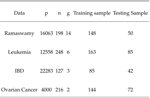
ii rameter. The third method assumes that groups share common eigenvector in eigenvector-eigenvalue decomposition of their within-group covariance matri-ces, while their eigenvalues my differ. The fourth method assumes the within-group covariance matrices are proportional to each other. The fifth method is derived from the Dantzig selector and uses optimal scoring to construct discrim-inant function. The third and fourth methods achieve sparsity by imposing a cardinality constraint with the cardinality level determined by cross-validation. All the new methods reduce their computation time by sequentially determining individual discriminant functions. The methods are applied to six real data sets and perform well when compared with two existing methods.
The accomplishment of this doctoral thesis would not have been possible with-out the support and encouragement of a number of people. I would like to ex-press my sincere gratitude to all of them. First of all, I am extremely grateful to my PhD supervisors: Prof. Paul Garthwaite, Dr. Nickolay Trindafilov, and Prof. Frank Critchley who are staff members of the school of Mathematics and Statistics, The Open University. I thank Prof. Paul Garthwaite, my first supervi-sor, for his valuable guidance, scholarly inputs and consistent encouragement I received throughout the research work, particularly in the last one year. This ac-complishment would not have been realized without his unconditional support and it was a great opportunity to do my doctoral programme under his guidance and to learn from his research expertise. I would also like to thank Dr. Nickolay Trindafilov, who was my first supervisor for the first 3 years of my PhD study, for all his guidance and unreserved scholarly supports in defining the research prob-lem, in suggesting directions and positive inputs so as to make my study feasible theoretically and practically. I would also like to thank Prof. Frank Critchley for his guidance and support as my second supervisor. He gave me fruitful com-ments to shape my PhD research works and the thesis.
iv I extend my gratitude to all staff members of the Statistics group at the Open University. To mention some of them: Dr Alvaro Faria, Prof Chris Jones, Dr. Catriona Queen, Dr. Karen Vines, Dr. Heather Whitaker, Prof. Kevin McConway, Prof. Paddy Farrington, and Dr. Fadlalla Elfaday. They were very kind enough to extend their help at various phases of this research, whenever I approached them, and I do hereby acknowledge all of them. I would also like to thank the Open University for funding my PhD study.
This is good opportunity to thank Dr. Ian Short, senior lecturer of Mathemat-ics at the Open University, for all his optimistic and continuous help and encour-agements during the difficult time in my studies. Related with this, my thank also goes to Prof. Uwe Grimm, Head of the school of Mathematics and Statistics, for his help to realize the completion of my PhD.
I thank Dr. Yonas Weldeselassie for his friendly and brotherly support in var-ious kinds from the beginning of the start of my PhD up to the completion of my PhD. I would also like to thank Saba Berhanu (wife of Dr Yonas) for her en-couragements. Similarly, I would like to thank Dr. Yoseph Nugusse and his wife (Selam) for their advices and encouragements.
Last but not least, I would like to thank my family members, friends, class-mates, officeclass-mates, and colleagues for their continuous encouragements through-out my PhD studies.
List of Publications v
Table of Contents v
List of Tables x
List of Figures xii
List of Abbreviations xiv
1 Introduction and preliminaries 1
1.1 Introduction . . . 1
1.2 Thesis outline . . . 7
2 The discriminant analysis framework 10 2.1 Discrimination and classification problems . . . 10
2.2 Basic notation and data organization . . . 11
2.3 Principles of classification and discrimination . . . 12
2.3.1 Classification into two groups. . . 12
2.3.2 Optimal allocation criteria . . . 15
Table of Contents vi
2.3.3 Classification into several groups . . . 18
2.4 Approaches to linear discriminant analysis . . . 19
2.4.1 Discrimination via multivariate normal models . . . 20
2.4.2 Fisher’s linear discriminant analysis . . . 24
2.4.3 Regression approach to LDA for two groups . . . 31
3 Review of discriminant analysis in high-dimensions 33 3.1 Dimension reduction Methods . . . 34
3.2 Regularization methods . . . 37
3.2.1 Independence assumption. . . 37
3.2.2 Dependence assumption. . . 46
3.3 Ratio optimization methods . . . 53
3.3.1 A gradient LDA. . . 54
3.3.2 Variable selection in discriminant analysis via the Lasso . . 55
3.3.3 A sparse LDA algorithm based on subspaces . . . 58
3.4 Optimal scoring methods . . . 61
3.4.1 Penalized discriminant analysis . . . 62
3.4.2 Sparse discriminant analysis . . . 64
3.4.3 A direct approach to LDA in ultra-high dimensions . . . 64
3.5 Miscellaneous methods. . . 66
3.5.1 Regularized optimal affine discriminant (ROAD) . . . 66
3.5.2 A direct estimation approach . . . 69
3.5.3 Sparse LDA by thresholding (SLDAT) . . . 71
3.6 Limitations of the existing high-dimensional discrimination methods 74
4 Function constrained sparse LDA 77
4.1 Introduction . . . 77
4.2 Sparse Linear Discriminant analysis . . . 79
4.3 Function constrained sparse LDA (FC-SLDA) . . . 81
4.3.1 General approach to FC-SLDA . . . 83
4.3.2 Sequential method of FC-SLDA. . . 86
4.3.3 Algorithm 1: FC-sparse LDA . . . 89
4.3.4 Interpretation and sparseness . . . 92
4.4 FC-SLDA without eigenvalues (FC-SLDA2) . . . 94
4.4.1 Algorithm 2: FC-SLDA2 . . . 95
4.5 Numerical applications . . . 96
4.5.1 Applications using small data sets . . . 97
4.5.2 Applications with high-dimensional data . . . 101
4.6 Results and discussion . . . 104
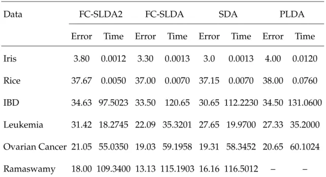
4.6.1 Comparison with exiting methods . . . 104
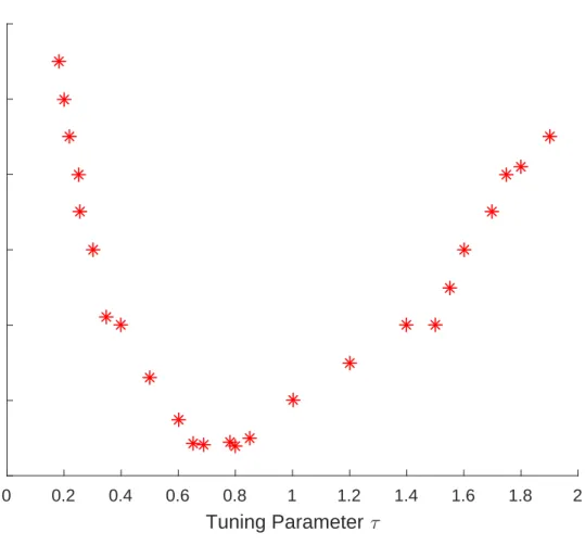
4.6.2 Choice of tuning parameter (τ) . . . 106
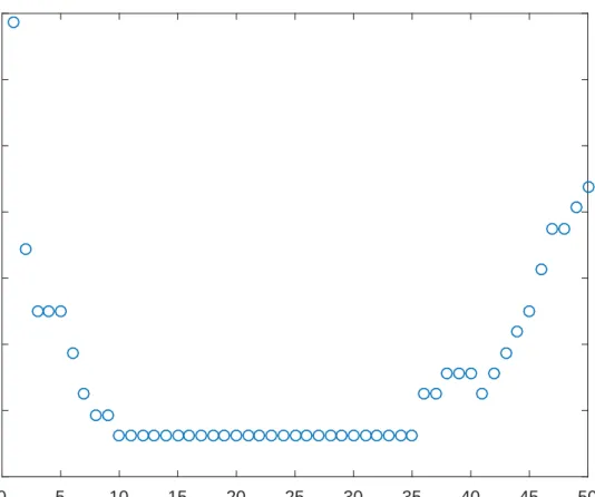
4.6.3 Variable selection and sparseness . . . 107
4.7 Chapter summary . . . 110
5 Sparse LDA using common principal components 111 5.1 Introduction . . . 111
5.2 Discrimination using common principal components . . . 114
Table of Contents viii
5.3.1 Likelihood approach to discriminant analysis . . . 117
5.4 Sparse LDA based on common principal components . . . 120
5.4.1 Sparsity using a cardinality constraint . . . 122
5.4.2 Algorithm 3: SDCPC . . . 123
5.5 Numerical illustrations . . . 125
5.5.1 Numerical Results of SDCPC on real data sets . . . 125
5.5.2 Comparison with other methods . . . 127
5.6 Sparse LDA using proportional CPC . . . 131
5.6.1 Maximum Likelihood estimation of proportional PCs . . . . 133
5.6.2 Least square estimation of proportional CPC . . . 134
5.6.3 Sparse discrimination using proportional CPC (SD-PCPC) . 138 5.6.4 Algorithm 4: SD-PCPC . . . 139
5.6.5 Numerical illustration of SD-PCPC. . . 141
5.7 Chapter summary . . . 144
6 Sparse LDA using optimal scoring 145 6.1 Introduction . . . 145
6.2 Connection of multivariate regression analysis and discriminant analysis via optimal scoring . . . 147
6.3 Linear discriminant analysis via optimal scoring . . . 150
6.4 Sparse LDA using optimal scoring . . . 152
6.4.1 Algorithm 5: SLDA-OS . . . 157
6.5 Numerical illustration . . . 159
6.5.2 Application to real data sets . . . 161
6.6 Chapter summary . . . 165
7 General conclusions and future research 167
7.1 Summary and conclusions . . . 167
7.2 Future research . . . 177
List of Tables
2.1 Multivariate data for discriminant analysis . . . 12
3.1 Number of parameters to estimate for constrained Gaussian models . . . 37
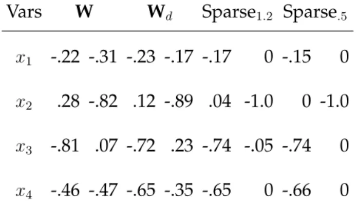
4.1 Different raw coefficients for Fisher’s Iris Data . . . 98
4.2 Summary of four high-dimensional datasets . . . 103
4.3 Misclassification rate (in %) and time ( in seconds) of four sparse LDA methods. The results were found using the testing data sets. . . 105
5.1 Numerical results of SDCPC on low and high-dimensional real datasets . 126
5.2 Classification error, time and sparsity of three methods . . . 130
5.3 Constants of proportionality of sample covariance matrices of real data sets141
5.4 Numerical results of SD-PCPC on low and high-dimensional real datasets 142
6.1 Misclassification rate (in %), time ( in seconds), and sparsity (in %) of two methods on the testing sets of three simulated data sets. . . 161
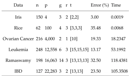
6.2 Misclassification rate (in %) and time ( in seconds) of three sparse LDA methods on the testing sets of six real data sets. . . 162
7.1 Assumptions about covariance matrices made by the five methods
pro-posed in this thesis. . . 170
7.2 Misclassification rate (in %) and time (in seconds) of seven sparse dis-criminant analysis methods on six real data sets. . . 176
List of Figures
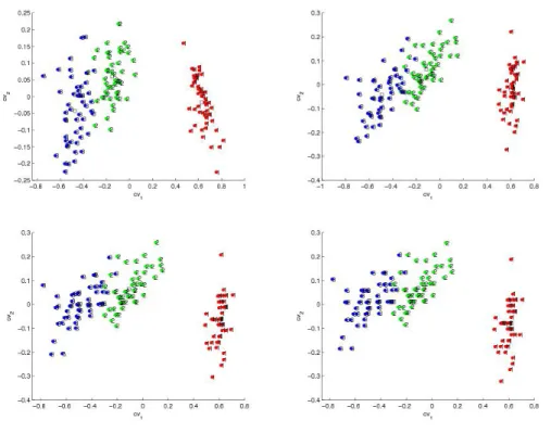
4.1 Iris data plotted against two CVs. 1=Iris setosa, 2=Iris versicolor, 3=Iris virginica. Squares denote group means. The(1,1)panel uses the original CVs (withW). The(1,2)panel uses the CVs withWd. The panels(2,1) and(2,2)use sparse CVs withτ = 1.2andτ = 0.5respectively. . . 99
4.2 Rice data plotted against two CVs. The groups are 1=France, 2=Italy, 3=India, 4=USA. Squares denote group means. The (1,1) panel uses the CVs withWd. The panels (2,1)and(2,2), and(3,1)and(3,2)use sparse CVs withτ =.5andτ =.01respectively. . . 101
4.3 Tuning parameter(τ)plotted against misclassification rate for the train-ing data set of the ovarian cancer data. The misclassification rate de-creases steadily whenτ increases from 0 to 0.6. The misclassification rate stabilizes and attains its minimum whenτ is between 0.6 and 0.9. Then the misclassification rate increases again forτ ≥1. . . 107
4.4 Classification error is plotted against the number of selected variables. . . 108
5.1 Classification error of training and testing samples is plotted against the number of variables for the Leukemia data. . . 128
5.2 Scatter plot of the three groups of IBD data (i.e. Normal, Crohns, and
Ulcerative) using two discriminant directions . . . 129
6.1 The misclassification rate of the training set of the ovarian cancer data for different values of the tuning parameter (λ) resulting from cross-validation of SLDA-OS method. . . 164
6.2 The misclassification rate of the training set of the Ramaswamy data for different values of the tuning parameterλresulted from cross-validation of SLDA-OS method. . . 165
List of Abbreviations
CPC Common Principal Components
DA Discriminant Analysis
FC-SLDA Function Constrained Sparse Linear Discriminant Analysis
LDA Linear Discriminant Analysis
LDF Linear Discriminant Function
ODE Ordinary Differential Equations
OS Optimal Scoring
PCA Principal Components Analysis
PLDA Penalized Linear Discriminant Analysis
QDA Quadratic Discriminant Analysis
SDA Sparse Discriminant Analysis
SDCPC Sparse Discrimination with CPC
SD-PCPC Sparse Discrimination with Proportional CPC
SLDA-OS Sparse Linear Discriminant Analysis with Optimal Scoring
Chapter 1
Introduction and preliminaries
1.1
Introduction
With the recent development of new technologies, high-dimensionality has become a common problem in various disciplines such as medicine and epidemi-ology, genetics, biepidemi-ology, metrepidemi-ology, astronomy, and economics. High-dimensionality is a situation where the number of variables (the dimension of the data vec-tors) is much larger than the number of observations (sample size) (Qiao et al.,
2009). Some sources of high-dimensional data are digital images, documents,
next-gen sequencing, mass spectrometry, metabolomics, microarray (gene ex-pression), proteomics, videos and web pages (Pang and Tong, 2012). The high-dimensionality problem, in general, occurs in many applications including infor-mation retrieval, character recognition, classification and microarray data analy-sis (Ye,2005).
To analyse high-dimensional data, many methods have been proposed for fast query response, such as K-D tree and R-tree (Cai et al., 2008). However, the
performance and efficiency of these types of methods decrease as the dimension-ality increases because the methods are designed to operate with small dimen-sionality. Consequently, dimension reduction, or variable selection, has become an important approach to deal with high-dimensional problems so as to obtain meaningful results. Once the high-dimensional data are transformed into a lower dimensional space, conventional data analysis methods can be employed (Cai et al., 2008). One of the most commonly used dimension reduction methods for
data with grouped observations is Discriminant Analysis (DA). Principal Com-ponent Analysis (PCA) is another popular method used for dimension reduc-tion. It helps to find a few directions on which to project the data such that the projected data explain most of the variability in the original data. This method finds a low dimensional representation of the data without losing much informa-tion. Although PCA can be used for dimension reduction, it is not appropriate for classification problems because it mainly works for unsupervised problems (Qiao et al.,2009).
Discriminant Analysis (DA) is generally defined as the study of the relation-ship between a categorical variable and a set of interrelated variables ( McLach-lan, 2004). A method that is commonly used together with DA is classification, which is a supervised method that deals with the problem of the optimal alloca-tion of a given set of objects into a predefined mutually exclusive and exhaustive classes. Fisher (1936) proposed a special type of DA called linear discriminant analysis (LDA). It is a method used in statistics, pattern recognition and machine learning to find a linear combination of variables, linear discriminant functions
CHAPTER1. INTRODUCTION AND PRELIMINARIES 3
(LDF), which characterize or separate two or more groups of objects or events. The resulting linear combination of variables may be used as a classifier, or, more commonly, for dimensionality reduction before classification. The main objective of LDA is to describe, either graphically (in few directions) or algebraically, the difference between two or more groups of objects as well as to perform dimen-sionality reduction while preserving as much of the class discriminatory infor-mation as possible (Johnson and Wichern,2002).
The classical Fisher’s LDA approach uses the class information to find infor-mative projections of the data for a classification problem. Fisher(1936) consid-ered the problem of finding a linear combination of variables that best discrim-inates groups by maximizing the ratio of between-class variance to within-class variance. In the case of two classes, the derived linear combination of variables is called a linear discriminant function (LDF), or canonical variate (Trendafilov and
Vines, 2009). In the same manner, additional LDF’s with decreasing importance in discrimination can be obtained sequentially (Qiao et al.,2009). This method of discrimination is further generalized byRao(1952) to the multiple class problem.
In general, when the number of variables is greater than the number of groups, the total number of discriminant functions that can be defined is one less than the number of groups. For example, when there are three groups, we could esti-mate two discriminant functions, one function for discriminating between group 1 and groups 2 and 3 combined, and another function for discriminating between group 2 and group 3.
follows a multivariate normal distribution with significantly different group means but a common covariance matrix (Merchante et al.,2012;Trendafilov and Jolliffe,
2007; Johnson and Wichern, 2002). Together with the minimization of the prob-abilities of misclassification, this basic normality assumption leads to a Bayes discrimination method that coincides with Fisher’s LDA. Alternatively, Fisher’s LDA can also be formulated as a linear regression model through the concept of optimal scoring of the classes (Mai et al.,2012; Clemmensen et al.,2011;
Mer-chante et al.,2012;Hastie et al.,1995).
It is well known that classical LDA is one of the dimension reduction methods that performs well when the number of observations to be classified is much larger than the number of variables used for discrimination and classification. However, in the high dimensional setting, that is, when the number of variables is much larger than the number of observations, classical LDA fails to perform classification effectively due to the following well known problems (Clemmensen et al., 2011; Fan et al., 2012; Witten and Tibshirani, 2011; Ng et al., 2011; Hastie et al.,1995).
1. The estimate of the within-group covariance matrix is singular.
2. The resulting discriminant functions are very difficult to interpret, because each discriminant function includes a linear combination of all of the origi-nal variables.
3. Computational cost in terms of both running time and storage is very ex-pensive.
CHAPTER1. INTRODUCTION AND PRELIMINARIES 5
Furthermore, many more problems of high-dimensional data have been identi-fied by various studies. For instance, Bickel and Levina (2004) pointed out that Fisher’s LDA performs poorly in a minimax sense due to the diverging spectra
frequently encountered in high-dimensional covariance matrices. Fan and Fan
(2008) also demonstrated that the difficulty in high-dimensional classification is due to the presence of redundant variables (noise accumulation) that do not signif-icantly contribute to the minimization of classification error or to the maximiza-tion of discriminamaximiza-tion between groups. Similarly,Qiao et al.(2009) stated that in high-dimensional discriminant analysis, most of the time data are projected onto various directions, many of the projections are exactly the same. That is, the data overlap on top of each other. They referred to this phenomenon asdata pillingor over fitting.
In general, many effective statistical techniques such as LDA cannot even be computed directly in high-dimensional data due to the aforementioned prob-lems. If LDA is directly applied to such data settings, it may provide meaningless results. Therefore, appropriate methods of transformation or dimension reduc-tion are required to apply LDA in such circumstances.
There exist several references that have proposed various methods to extend classical LDA to overcome the problems that arise in the high-dimensional set-ting. Recently proposed extensions of LDA focus mainly on dimension reduction through variable selection and on the estimation of the inverse of the within-class covariance matrix by applying different regularization techniques (Clemmensen
Fan,2008;Ng et al.,2011).
Variable selection is an approach by which high-dimensional data is reex-pressed in terms of fewer variables while minimizing the loss of necessary infor-mation for discrimination (Merchante et al., 2012; Hastie et al., 1995). The
vari-ables obtained after the final dimension reduction process are commonly called discriminant variables (Hastie et al.,1995). The main purpose of variable selec-tion is to achieve sparsity. Sparsity is a situaselec-tion where the discriminant vectors have only a small number of nonzero components (Qiao et al., 2009). In other words, sparse LDA produces linear discriminant functions with only a small number of variables, retaining those variables that are important in discrimi-nating between groups and in identifying group membership of observations. In high-dimensional data analysis, such as most genetic analyses, sparse meth-ods of discrimination ensure better interpretability, robustness of the model, or less computational cost for prediction (Clemmensen et al.,2011;Merchante et al.,
2012).
Variable selection is an essential procedure in the derivation of sparse LDA. In high-dimensional data, often a large number of variables on which measure-ments are observed are available for analysis, while few of these variables contain useful information for the purpose of classification (Rencher, 2002). Qiao et al.
(2009) pointed out that we do not necessarily ensure an increase in the discrimi-natory power by increasing the number of variables in the application of Fisher’s LDA. Instead it leads to formation of overfitting. Since the 1990’s, a number of techniques have been proposed for variable selection with high-dimensional
CHAPTER1. INTRODUCTION AND PRELIMINARIES 7
data. The prominent methods are variable selection via the Lasso (Tibshirani,
1996), variable selection via the elastic net (Zou and Hastie, 2005), the Dantzig selector (Cand`es and Tao, 2007), and the group Lasso (Merchante et al., 2012). The traditional approach to sparse LDA is performing variable selection in a sep-arated step before classification. However, this approach leads to a dramatic loss of information for the purpose of the overall classification problem (Filzmoser et al., 2012). Therefore, there is a need to develop a sparse LDA method that
performs variable selection and classification simultaneously.
1.2
Thesis outline
Each of the chapters in this thesis can be read as a self-contained article. In general, the thesis is organized as follows. Chapter2briefly introduces the
gen-eral discriminant analysis framework. Various techniques of classical discrim-inant analysis are presented to give a general background about discrimdiscrim-inant analysis. The principles of classification and discrimination are presented here. Moreover, three approaches to discriminant analysis are presented in this chap-ter. These are discrimination via multivariate normal models, Fisher’s LDA, and the regression approach to LDA.
Chapter 3 reviews some of the existing discriminant approaches in high di-mensional settings. This chapter, in general, reviews the approaches that focus on dimension reduction, regularization of the within-groups sample covariance matrix, minimization of classification error, and other direct methods. With these approaches, ordinary LDA is used after dimension reduction. Other methods
that are reviewed in Chapter 3are methods that assume the variables in a
high-dimensional data are independent.
Chapter 4 proposes a method called function-constrained sparse LDA (FC-SLDA) and its simplified version, FC-SLDA2, that are alternative methods for high-dimensional discriminant analysis. The constrained`1-minimization penalty
is imposed on the discrimination problem to achieve sparsity, and FC-SLDA im-poses a diagonal within-group covariance matrix to circumvent the singularity problem. The second method proposed in this chapter, FC-SLDA2, is derived without using eigenvalues. Both methods are illustrated using real data sets. They are also compared with other exiting methods.
Chapter5starts by introducing a new method of discrimination called sparse LDA using Common principal components (CPC) and then continues with the theoretical development of the method. Sparse discriminant method using CPC (SDCPC) assumes that group covariance matrices have the same eigenvectors but different eigenvalues. It is an effective method for high-dimensional classifica-tion problems. This method is illustrated by using real data sets. Finally, Chap-ter 5 proposes another alternative sparse discrimination method called sparse LDA using proportional CPC (SD-PCPC) for high-dimensional discrimination problems. This method is appropriate when group covariance matrices are pro-portional to each other.
Chapter 6proposes a new formulation to sparse LDA method based on op-timal scoring named as SLDA-OS. This discrimination method is derived by re-casting discriminant analysis as regression analysis. The Danzig selector is
incor-CHAPTER1. INTRODUCTION AND PRELIMINARIES 9
porated within this method to achieve sparsity of the discriminant functions. The thesis ends with summary and conclusions in Chapter 7, where each chapter is briefly summarized, results are discussed, and conclusions are pre-sented. Some future research directions are also indicated in this chapter. We used MATLAB2015b to implement the algorithms of our methods.
The discriminant analysis framework
In this chapter, we outline the general framework (formulation) of the discrimina-tion problem and present the main approaches of classical discriminant analysis.
2.1
Discrimination and classification problems
Discriminant analysis and classification are multivariate techniques concerned with separating distinct sets of objects and with allocating new objects to previ-ously defined groups. Discriminant analysis is a dimension reduction method that is useful in determining whether a set of variables is effective in predicting group membership. For example, linear discriminant analysis (LDA) is used to identify a linear combination of variables, called the linear discriminant func-tion, that produces the greatest distance between groups. A restriction on using standard LDA is that it requires group covariances to be equal. Some other non-linear discriminant analysis, such as quadratic discriminant analysis (QDA), may be used when the group covariances are not equal.
CHAPTER2. THE DISCRIMINANT ANALYSIS FRAMEWORK 11
The goal of discrimination, in general, is to describe the differential features of objects that can be used to separate the objects into groups as well as to pre-dict group membership of further objects (Fisher, 1936). The latter task overlaps classification analysis which is concerned with the development of rules for allo-cating or assigning observations into one or more already existing groups.
Because linear discriminant functions are often used to develop classification rules, some authors use the term classification analysis instead of discriminant analysis. Because of the close association between the two processes we treat them together in this subsection.
2.2
Basic notation and data organization
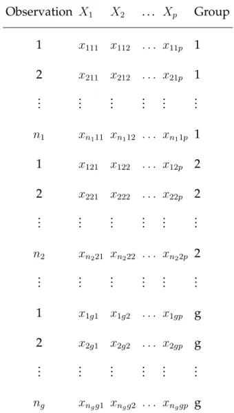
Multivariate data for discriminant analysis arise when measurements made on p variables are recorded for a total of n observations (individuals). Because we are now dealing with classical LDA, we assume that n > p. Suppose that thenobservations are divided intogpredefined groups and that theithgroup is denoted byπi,i= 1,2, . . . , g. Ifni is the number of observations in theithgroup,
thenn1+n2+· · ·+ng =n. Let the(p×1)vectorxij = (xij1, xij2, . . . , xijp)T denote
the measurement made on thejth individual belonging to theith group, and let the(n×p)data matrixXrepresent the measurements of all observations. Values will be available forpvariablesX1, X2, ..., Xpfor each observation. Thus, the data
for discriminant analysis takes the form shown in Table2.1.
Therefore, the matrix X contains the data consisting of all of the n obser-vations on all of the p variables in g groups. It can also be given as XT =
Table 2.1: Multivariate data for discriminant analysis Observation X1 X2 . . . Xp Group 1 x111 x112 . . . x11p 1 2 x211 x212 . . . x21p 1 .. . ... ... ... ... ... n1 xn111 xn112 . . . xn11p 1 1 x121 x122 . . . x12p 2 2 x221 x222 . . . x22p 2 .. . ... ... ... ... ... n2 xn221 xn222 . . . xn22p 2 .. . ... ... ... ... ... 1 x1g1 x1g2 . . . x1gp g 2 x2g1 x2g2 . . . x2gp g .. . ... ... ... ... ... ng xngg1 xngg2 . . . xnggp g [X1, X2, ..., Xp].
2.3
Principles of classification and discrimination
2.3.1
Classification into two groups
Suppose the overall set of measurements on n observations is divided into two groups. The first group isπ1 and containsn1observations; the second group π2 containsn2observations. Let these two populations be described by
probabil-CHAPTER2. THE DISCRIMINANT ANALYSIS FRAMEWORK 13
ity density functionsf1(x)andf2(x), respectively, where the observed values of
xdiffer to some extent from one group to the other (Johnson and Wichern,2002). An observation with associated measurementsx, must be assigned to either
π1 orπ2. LetΩbe the sample space; that is, the collection of all possible
observa-tions x. The space is divided into two regions, say, R1 and R2 = Ω−R1. If an
observation falls in R1, we classify it as belonging to π1, and if the observation
falls in R2, we classify it as belonging to π2. Since every observation must be
assigned to one and only one of the two populations, the regions R1 and R2 are
mutually exclusive and exhaustive (Johnson and Wichern,2002).
In using any classification procedure, two types of errors can be committed: an observation may be incorrectly classified as coming from π2 when, in fact, it
is fromπ1, and viceversa (Anderson,1984). The principle of optimal allocation is
to create a rule (R1andR2) that minimizes the chances of making these errors. In
general, a large number of observations tend to be classified into their respective groups.
With good classification method, the chances or probabilities of misclassifica-tion should be small. The condimisclassifica-tional probability of classifying an object as π2
when , in fact, it is fromπ1is given as :
p(2|1) =p(X ∈R2|π1) = Z
R2
f1(x)dx (2.1)
Similarly, the conditional probability of classifying an object asπ1when it is really
fromπ2 is
p(1|2) =p(X ∈R1|π2) = Z
R1
f2(x)dx (2.2)
overall probabilities of correctly or incorrectly classifying objects can be derived as the product of the prior and conditional classification probabilities.i.e.,
p(correctly classified as π1) = p(X ∈R1|π1).p(π1) = p(1|1).p1 (2.3)
and
p(misclassified asπ1) =p(X∈R1|π2).p(π2) =p(1|2).p2 (2.4)
In the same manner, the probabilities of correctly and incorrectly classifying ob-servations asπ2 are given as , respectively:
p(X∈R2|π2).p(π2) =p(2|2).p2 (2.5)
and
p(X∈R2|π1).p(π1) = p(2|1).p1. (2.6)
Classification methods are often evaluated based on their probabilities of mis-classification (PoM). A mis-classification procedure with smaller PoM is said to be better than another method of classification with larger PoM. Consequently, in the case of two groups classification process, the idea of classification is to de-velop a method that minimizes the PoM’s in equations2.4and2.6.
Another criteria for classification is cost. Suppose that classifying aπ1
obser-vation wrongly toπ2 represents a more severe error than classifying aπ2
obser-vation wrongly toπ1. Then one should be cautious about committing the former
error. Let the cost of an observation fromπ1 is misclassified asπ2 bec(2|1), and
the cost of an observation fromπ2 is misclassified asπ1 bec(1|2). Then the
aver-age or expected cost of misclassification (ACM) is given as:
CHAPTER2. THE DISCRIMINANT ANALYSIS FRAMEWORK 15
It is noted inJohnson and Wichern(2002) that the cost for correct classification is
zero. A reasonable classification rule aims to have an ACM as small as possible.
2.3.2
Optimal allocation criteria
Many different optimal allocation criteria have been proposed to determine a classification rule. One criterion is to obtain a classification rule by minimizing the ACM. A procedure that minimizes (2.7) for givenp1 andp2 is called a Bayes
rule (Anderson,1984). The regionsR1andR2that minimize the ACM are defined
by the valuesxfor which the following inequalities hold
R1 : f1(x) f2(x) ≥ c(1|2) c(2|1) p2 p1 , (2.8) and R2 : f1(x) f2(x) < c(1|2) c(2|1) p2 p1 . (2.9)
If the misclassification cost ratio is unknown, it is commonly taken to be unity and the population density ratio is compared with the ratio of the prior probabil-ities. Suppose for a moment thatc(1|2) = c(2|1) = 1. Then the expected cost of misclassification (the ACM) given in (2.7) becomes solely a function of the prob-abilities. As a result, we call it the total probability of misclassification (TPM), given as : TPM = p1.p(2|1) +p2.p(1|2) = p1 Z R2 f1(x)dx+p2 Z R1 f2(x)dx = p1 1− Z R1 f1(x)dx +p2 Z R1 f2(x)dx = p1+ Z R1 [p2f2(x)−p1f1(x)]dx. (2.10)
This quantity is minimized if R1 is chosen so that p2f2(x)−p1f1(x) < 0 for
all points in R1. Minimizing (2.10) is mathematically equivalent to minimizing
the expected cost of misclassification when the costs of misclassification are equal (Johnson and Wichern,2002). The classification rule that minimizes TPM is given
as follows: Assign an observationxtoπ1if f1(x) f2(x) ≥ p2 p1 ; (2.11)
otherwise assign it to π2. Moreover, when the prior probabilities are unknown,
they are taken to be equal, i.e., p1 = p2 = 1/2. Under both conditions, the
opti-mal classification regions are determined simply by comparing the values of the density functions. Hence, with the assumption of equal cost of misclassification and equal prior probabilities, we assign an observationxtoπ1iff1(x)/f2(x)≥1,
otherwise we assign it toπ2.
Another optimality criterion that leads to the assignment rule in (2.11) is based on posterior probability. Using this approach an observationxis allocated to the group with the largest posterior probability p(πi|x). By Bayes rule, the
posterior probability ofπiis given as:
p(πi|x) = p(x|πi)p(πi) P2 k=1p(x|πk)p(πk) = pifi(x) p1f1(x) +p2f2(x) , i= 1,2. (2.12)
An observation xis assigned toπ1 when p(π1|x) > p(π2|x), this is equivalent to
the rule that minimizes the total probability of misclassification.
misclassi-CHAPTER2. THE DISCRIMINANT ANALYSIS FRAMEWORK 17
fication should be minimized. This criterion is commonly known as theminimax
rule. Thus, the minimax rule allocates an observation x so as to minimize the greater of p(1|2) and p(2|1) (Lachenbruch, 1975; Seber, 2004). For instance, for
0≤α≤1,
max{p(1|2), p(2|1)} ≥(1−α)p(2|1) +αp(1|2) (2.13) By (2.11) the right hand side of (2.13) is minimized whenR1 =R01={f1(x)/f2(x)≥ α/(1−α) =c}. If we choosec, sayα =α0, so that the misclassification
probabil-ities forR01are equal, that is,p0(2|1) =p0(1|2), then
(1−α0)p(2|1) +α0p(1|2) ≥ (1−α0)p0(2|1) +α0p0(1|2) = (1−α0+α0)p0(2|1)
= p0(2|1)
Therefore, (2.13) can be given as,
max{p(1|2), p(2|1)} ≥p0(2|1) = max{p0(1|2), p0(2|1)}.
Thus, the minimax rule is: Assign x to π1 if f1(x)/f2(x) ≥ c, where c satisfies p0(1|2) =p0(2|1).
If the two groups are normal with common covariance matrix, then the mini-max rule is given as: Assign an observationxtoπ1if
D(x)≥lnc,
where D(x) is given by (2.21). The minimax rule is the same as the maximum likelihood ratio method whenlnc = 0orc = 1. Both allocation methods do not require knowledge ofp1.
2.3.3
Classification into several groups
Here the principles of classification presented in the previous sections will be extended to the case where there are more than two groups. Let the observations be divided into g groups, where theith group is denoted byπi with associated
density functions fi(x), i = 1,2, . . . , g. The space of observations is assumed
to be divided into g mutually exclusive and exhaustive regions R1, R2, . . . , Rg.
Let pi be the prior probability of πi, and let c(k|i) be the cost of assigning an
observation wrongly to πk when, in fact, it belongs to πi fori 6= k = 1,2, . . . , g.
For k = i, c(i|i) = 0. Similarly, letp(k|i)be the probability of misclassifying an observation toπkwhen, in fact, it comes fromπi, which is given as:
p(k|i) = Z Rk fi(x)dx for i, k = 1,2, . . . , g. (2.14) with p(i|i) = 1− g X k=1 k6=i p(k|i)
The conditional expected cost of misclassifying an observationxfromπ1 toπ2 or π3, . . . , orπg is: ACM(1) = p(2|1)c(2|1) +p(3|1)c(3|1) +· · ·+p(g|1)c(g|1) = g X k=2 p(k|1)c(k|1). (2.15)
The conditional expected costs of misclassification for the other groups can also be obtained from equivalent formula. Multiplying each conditional expectation
CHAPTER2. THE DISCRIMINANT ANALYSIS FRAMEWORK 19
by its prior probability and summing the results gives the overall ACM:
ACM = g X i=1 pi g X k=1,k6=i p(k|i)c(k|i) ! . (2.16)
Determining an optimal classification procedure means choosingRK, k = 1,2, . . . , g
so that (2.16) is minimized. The allocation rule is: Assignxtoπk, k = 1,2, . . . , g
for which (2.16) is smallest (Johnson and Wichern, 2002). If all the misclassifi-cation costs are equal, the minimum ACM and the minimum TPM are the same and, without loss of generality, we can set all the misclassification costs equal to 1. This assumption leads to the allocation rule that we would allocatexto group
πk, k= 1,2, . . . , g, for which
g
X
i=1,i6=k
pifi(x) (2.17)
is smallest. Note that equation (2.17) will be smallest when the omitted term,
pkfk(x), is largest. As a result, when all the misclassification costs are the same,
the allocation rule is that we assignxtoπkifpkfk(x) > pifi(x)for alli 6= k. It is
important to note that this classification rule is identical to the one that maximizes the posterior probabilityp(πk|x), where
p(πk|x) =
pkfk(x)
Pg
i=1pifi(x)
fork = 1,2, . . . , g. (2.18)
Equation (2.18) is the generalization of equation (2.12) forggroups.
2.4
Approaches to linear discriminant analysis
There are many approaches to LDA. In this section, we will present three ap-proaches, namely, multivariate normal discrimination, Fisher’s discrimination, and discrimination using regression approach.
2.4.1
Discrimination via multivariate normal models
2.4.1.1 Discrimination with two multivariate normal populations
Here we assume that f1(x) and f2(x) are multivariate normal densities; the
first with mean vector µ1 and covariance matrix Σ, and the second with mean vector µ2 and the same covariance matrix, Σ. We also assume that all of the population parameters are known. The multivariate normal density of xT = [x1, x2, ..., xp]for theithgroup is:
fi(x) = 1 (2π)p/2|Σ|1/2 exp[− 1 2(x−µi) TΣ−1 (x−µi)], i= 1,2. (2.19)
Thus, the ratio of the densities is:
f1(x) f2(x) = exp[− 1 2(x−µ1)TΣ−1(x−µ1)] exp[−1 2(x−µ2)TΣ−1(x−µ2)] = exp[(µ1−µ2)TΣ−1x−1 2(µ1−µ2) T Σ−1(µ1+µ2)] (2.20) Taking logarithm the optimal rule becomes: Assignxtoπ1if
D(x) = (µ1−µ2)TΣ−1(x−1
2(µ1+µ2))>ln p2 p1
; (2.21)
otherwise assignxtoπ2. Note that the inequality in (2.21) is found when the costs
of misclassification are assumed to be equal. Moreover, when p1 = p2 = 1/2, x
will be assigned toπ1 ifD(x)>0. D(x)can be rewritten as:
D(x) =wT(x−1
2(µ1 +µ2)) (2.22)
where w =Σ−1(µ1 −µ2). It is important to see thatD(x)is a linear function of the observation vector xand hence it is known as the linear discriminant
func-CHAPTER2. THE DISCRIMINANT ANALYSIS FRAMEWORK 21
tion (LDF). In fact, wT in (2.22) is a row vector which can be given as, wT = (w1, w2, . . . , wp). For example, if an observation x0 consists of(x01, x02, . . . , x0p),
then the discriminant score,D(x), is computed as:
D(x0) =w0+w1x01+w2x02+· · ·+wpx0p
where w0 is a constant given byw0 = 12(µ1 −µ2)TΣ −1(µ
1+µ2)(Rencher, 2002; Johnson and Wichern,2002).
Whenp1 =p2 = 1/2, we assignxtoπ1 if wTx≥ 1 2(µ1 −µ2) TΣ−1 (µ1+µ2) = 1 2(w Tµ 1+wTµ2) (2.23)
This means that we assignxtoπ1 ifwTxis closer towTµ1than towTµ2.
To find the probabilities of misclassification, it is useful to know the distribu-tion of D(x). First, let us define the squared Mahalanobis distance between µ1
andµ2as
∆2 = (µ1−µ2)TΣ−1(µ1−µ2) =wT(µ1−µ2). (2.24) The distribution of D(x) is derived as follows. Since x is multivariate normal,
D(x)is also normal. This is becauseD(x)is a linear combination ofx. Ifxcomes fromπi(i= 1,2), the mean ofD(x)is
E[D(x)|πi] = E[(µ1 −µ2) TΣ−1 (xi− 1 2(µ1+µ2))] = (µ1−µ2)TΣ−1(µi− 1 2(µ1+µ2)) = 1 2(−1) i+1∆2. (2.25)
In either population the variance (var) is
var(D(x)) = var(wT(x− 1
2(µ1+µ2)))
Thus the probability of misclassification if the observation is fromπ1isp(2|1) = Φ({lnp2
p1−
∆2
2 }/∆), whereΦ(.)denotes the standard normal distribution function.
Similarly,p(1|2) = Φ(−{lnp1
p2 +
∆2
2 }/∆). If we assume thatp1 =p2 = 1/2, then p(2|1) =p(1|2) = Φ −∆ 2 ; (2.27)
and the total probability of misclassification is given as
T P M = 1 2p(D(x)<0|π1) + 1 2p(D(x)>0|π2) = 1 2Φ −∆ 2 +1 2Φ −∆ 2 = Φ −∆ 2 = 1−Φ ∆ 2 . (2.28)
The allocation principle is to find a classifierD(x)that minimizes the total prob-ability of misclassification in (2.28).
If the assumption of equal population variances was violated, the function would be a quadratic discriminant function (details are given inAnderson(1984)).
In such circumstances, quadratic discriminant analysis controls the variability in each group and provides reliable results.
2.4.1.2 Discrimination with several multivariate normal populations
Letfi(x)be a multivariate normal density function ofxfor populationπiwith
mean vectorµi and covariance matrix Σi, i = 1,2,· · · , g. LetΣbe the common
covariance matrix of theg populations under the assumption of homoscedastic-ity. The multivariate normal density ofxfor theithpopulation is
fi(x) = 1 (2π)p/2|Σ|1/2 exp −1 2(x−µi) T Σ−1(x−µi) , i= 1,2,· · · , g (2.29) Multiplying bypiand taking logarithm gives
Di(x) = lnpifi(x) = lnpi− p 2ln(2π)− 1 2ln|Σ| − 1 2(x−µi) TΣ−1 (x−µi) (2.30)
CHAPTER2. THE DISCRIMINANT ANALYSIS FRAMEWORK 23
Thus we assign x to πk if Dk(x) = max lnpifi(x), i = 1,2, . . . , g. The constant
term (p2) ln(2π)in (2.30) is the same for all groups. Hence, it can be ignored for allocation purposes. Similarly, we can ignore other terms that are the same for eachDi(x). Consequently, the final linear discriminant score for theithgroup can
be defined as Di(x) = lnpi+µTiΣ −1 x−1 2µ T i Σ −1 µi = lnpi+µTiΣ −1 (x− 1 2µi) (2.31)
We assignxto the group with the largest value ofDi(x).
It is important to note that the linear discriminant scores ing groups can also be expressed as:
Dik(x) = (µi−µk)
TΣ−1(x−1
2(µi+µk)) for i, k= 1,2, . . . , g, and i6=k. (2.32)
where Dik(x) is the discriminant function related to theith and kth groups, and
Dik(x) = −Dki(x). The regionRiis bounded by a(g−1)dimensional hyperplane.
The mean and variance of Dik(x) are, respectively, 12∆2ik and ∆2ik, where ∆2ik is
given as
∆2ik = (µi−µk)TΣ−1(µi−µk) = wikT(µi−µk), (2.33) wherewik =Σ−1(µi−µk).
When the population parameters are unknown, they can be replaced by their sample counterpart plug-in estimates. The sample mean vector and covariance
matrix for theith(i= 1,2, ..., g)group are given by ˆ µi = ¯xi = 1 ni ni X j=1 xij ˆ Σi = Si = 1 ni−1 ni X j=1 (xij−x¯i)(xij −x¯i)T (2.34)
Similarly, Σmay be estimated by the pooled sample covariance which is given by ˆ Σ=S= Pg i=1(ni−1)Si n−g (2.35)
And the overall mean vectorµis estimated as:
ˆ µ= ¯x= 1 n g X i=1 ni X j=1 xij (2.36)
2.4.2
Fisher’s linear discriminant analysis
Fisher’s approach does not assume normality, but it assumes that the popula-tions have equal covariance matrices. A pooled estimate of the covariance matrix will be used in this section. Similarly, sample estimates of the mean vectors will be used here.
It is convenient to start with two groups. Fisher(1936) determined the linear combination ofpvariables
y=aTx=a1x1+a2x2 +...+apxp (2.37)
that maximizes the distance between the two group mean vectors. This linear combination transforms the multivariate observations x to univariate observa-tions (scalar) y such that the y0s derived from populations π1 and π2 are
CHAPTER2. THE DISCRIMINANT ANALYSIS FRAMEWORK 25
standardized distance between the two group means, which is given as
[aT(¯x
1−x¯2)]2
aTSa = (¯x1−x¯2) T
S−1(¯x1 −x¯2) = ˆ∆2. (2.38)
The maximum of (2.38) is obtained when a = S−1(¯x1 −x¯2), or when it is any
multiple ofS−1(¯x1 −x¯2) (Rencher, 2002). Consequently, the linear combination
in (2.37) can be rewritten asy = (¯x1−x¯2)TS−1x. This function is called Fisher’s
linear discriminant function. It is identical to the standard LDA function (wTx)
with w =Σ−1(µ1 −µ2))given in Section2.4.1.1, but with unknown population means replaced by sample means. It can be shown that the maximizing vector
a is not unique because any multiple ofa = S−1(¯x1 −x¯2)will maximize (2.38).
However, its direction is unique. (Rencher,2002, p.271).
To extend Fisher’s approach of LDA tog groups, we first need to define the between-group and within-group covariance matrices. Let B be the between-groups covariance matrix and W be the within-groups covariance matrix ofX, which are given by
B= ˆΣb = 1 g−1 g X i=1 ni(¯xi−x¯)(¯xi−x¯)T and W= ˆΣw = 1 n−g g X i=1 ni X j=1 (xij −x¯i)(xij −x¯i)T. (2.39)
We seek a linear combination of the original variables that transforms the p -dimensional vector x to s-dimensional vector y, with s < p. The linear com-bination may be given as y = ATx, where A is a p×s transformation matrix
that gives the greatest discrimination between groups by maximizing the ratio of the between-groups covariance matrix to the within-groups covariance matrix of
the data (Trendafilov and Vines, 2009). Supposea1,a2, . . . ,as be respectively the
s column vectors of the transformation matrix A. The vectors a1,a2, . . . ,as are
obtained fromBandWsequentially as follows. Leta=a1, then it can be shown that (Trendafilov and Vines, 2009; Rencher, 2002; Johnson and Wichern, 2002) a
maximizes the following ratio:
aTBa
aTWa (2.40)
This maximization problem (2.40) is equivalent to the generalized eigenvalue problem given by
(B−λW)a=0 ⇒(W−1B−λIp)a=0. (2.41)
The solution to this equation is the eigenvalue of W−1B. Consequently, the largest eigenvalue, λ1, of W−1B, associated with the eigenvector a = a1, is the
maximum value of (2.40). The linear combinationaT1xis called the first linear
dis-criminant function. This disdis-criminant function is the most powerful disdis-criminant function. The second powerful discriminant function is given by the linear com-bination a>2x, where a2 maximizes the ratio (2.40) subject to Cov(a>1x,a>2x) = 0.
In general, the kth linear discriminant function is given by the kth linear
combi-nationa>
kx whose coefficient is associated with thekth eigenvector ofW
−1 B. ak
maximizes the ratio (2.40) subject to Cov(a>kx,ai>x) = 0, i < k, and Var(a>i x) =
1, i = 1, . . . , s. The power of discrimination of the linear combinations is deter-mined by their eigenvalues associated with their respective vector of coefficients. We consider the eigenvalues to be ranked as λ1 > λ2 > · · · > λs. The number
of (nonzero) eigenvalues s is the rank of B which is the minimum of (g −1, p). Hence the discriminant function that best separates the group means isy1 =aT1x.
CHAPTER2. THE DISCRIMINANT ANALYSIS FRAMEWORK 27
Subsequently, the remaining discriminant functions ordered in decreasing their power of discrimination are: y2 =aT2x, . . . , ys =aTsx. From theseigenvectors, we
obtain sdiscriminant functions (Rencher, 1992, section 8.4). These discriminant functions are uncorrelated, but they are not orthogonal. This is becauseW−1Bis not symmetric matrix.
The main objective of Fisher’s discriminant analysis is to separate groups. However, it can also be used to classify observations into their respective groups. The assumption of multivariate normality of the g-groups is not necessary to use Fisher’s discriminant method. But, the assumption that group covariance matrices are equal and full rank must be fulfilled. That is,Σ1 =Σ2· · ·=Σg =Σ.
Let λ1 ≥ λ2 ≥ · · · ≥ λs > 0denote the s ≤ min(g −1, p)nonzero
eigenval-ues of W−1Band let e1,e2, . . . ,es be the corresponding eigenvectors that satisfy
e>We = 1. Fisher’s LDA is obtained by finding a vector of coefficients a that maximizes (2.40).
The vector that maximizes (2.40) is given by a1 = e1. The linear combina-tion aT1Xis called the first linear discriminant function. This discriminant
tion is the most powerful discriminant function. The second discriminant func-tion is given by the linear combinafunc-tiona>2X, wherea2 = e2 maximizes the ratio (2.40) subject to Cov(a>1X,a>2X) = 0. In general, thekth linear discriminant
func-tion is given by the kth linear combination a>
kX whose coefficient is associated
with the kth eigenvector ofW−1B. ak = ek maximizes the ratio (2.40) subject to
Cov(a>kX,a>i X) = 0, i < k, and Var(a>i X) = 1, i= 1, . . . , s. The power of
eigenvec-tors. Hence, a1,a2, . . .as give discriminant functions, respectively ranked from
highest to lowest degree of discrimination.
Proof. We first convert the maximization problem to one already solved. By the spectral decomposition,Wcan be given asW=P>ΛPwherePis a matrix whose columns are the normalized eigenvectorse1,e2, . . . ,ek, and Λis a diagonal
ma-trix given as Λ= λ1 0 · · · 0 0 λ2 · · · 0 .. . ... . .. ... 0 0 · · · λk withλi >0.
LetΛ1/2 denote the diagonal matrix with elements√λi. Thus the symmetric
square-root matrix W1/2 = P>Λ1/2P and its inverse W−1/2 = P>Λ−1/2P satisfy
W1/2W1/2 = W, W1/2W−1/2 = I = W−1/2W1/2 andW−1/2W−1/2 =W−1. Now, let us set
b=W1/2a
sob>b=a>W1/2W1/2a=a>Waandb>W−1/2BW−1/2b=a>W1/2W−1/2BW−1/2W1/2a= a>Ba. Consequently, the maximization problem (2.40) can be reformulated as
max
b
b>W−1/2BW−1/2b
b>b . (2.42)
The maximum of this ratio is the largest eigenvalue ofW−1/2BW−1/2, which isλ1.
This maximization occurs when b = e1, the normalized eigenvector associated
with λ1. Because e1 = b = W1/2a1, or a1 = W−1/2e1, Var(a>1X) = a >
CHAPTER2. THE DISCRIMINANT ANALYSIS FRAMEWORK 29 e>1W −1/2 WW−1/2e1 = e>1W −1/2 W1/2W1/2W−1/2e1 = e>1e1 = 1. b ⊥ e1 maximizes
the preceding ratio whenb = e2, the normalized eigenvector corresponding to
λ2. For this choice,a2 =W−1/2e2, and Cov(a>1X,a > 2X) =a > 2Wa1 =e > 2e1 = 0, since e2 ⊥ e1. Similarly, Var(a>2X) = a>2Wa2 = e>2e2 = 1. We continue in this fashion
to determine the remaining discriminant functions. For example, to determine the kth discriminant, we find b ⊥ e
i that maximizes the ratio (2.42), subject to
orthogonality constraint, and this is the normalized eigenvector corresponding toλk. That is,b = ek, i < k. For this choice, the discriminant vector is given as
ak =W−1/2ek, and a>kWai = 1, i=k, for i, k = 1,2, . . . s 0, i < k.
Note that ifλis the eigenvalue ofW−1/2BW−1/2 andeis its associated eigen-vector , thenW−1/2BW−1/2e=λeand multiplying on the left hand side byW−1/2
gives
W−1/2W−1/2BW−1/2e=λW−1/2e or W−1/2B(W−1/2e) =λ(W−1/2e).
Consequently,W−1/2Bhas the same eigenvalues asW−1/2BW−1/2, but the corre-sponding eigenvector is proportional toW−1/2e=a, as shown above.
Let thekthlinear discriminant function (LDF) be given byYk =a>kX, where ak =W−1/2bk = ak1 ak2 .. . akp , and X= X1 X2 .. . Xp , k = 1,2, . . . s. (2.43)
Then the resultingslinear discriminantsY1, Y2, . . . , Ysare given as:
Y1 = a>1X=a11X1+a12X2+· · ·a1pXp (2.44)
Y2 = a>2X=a21X1+a22X2+· · ·a2pXp
.. . = ...
Ys = a>sX=as1X1+as2X2 +· · ·aspXp.
We can put these functions in matrix form as
Y= Y1 Y2 .. . Ys = a>1X a>2X .. . a>sX =A>X, (2.45)
where A is a transformation matrix whosekth row is a>
k such that AWA
> = Is.
This implies that the components ofYhave unit variances and zero covariances. The aim of deriving these discriminant functions is to obtain a low-dimensional representation of the data that separates the groups as much as possible. In addi-tion to group separaaddi-tion, the discriminants also give the basis for a classificaaddi-tion rule. A reasonable classification rule is one that assignsyto groupkif the square of the distance from ytoµk is smaller than the square of the distance fromyto
CHAPTER2. THE DISCRIMINANT ANALYSIS FRAMEWORK 31
It is well known thatWis singular when p >> n. Consequently, in the high-dimensional scenario, it is impossible to find the eigenvalues and their associated eigenvectors ofW−1B.
2.4.3
Regression approach to LDA for two groups
Fisher (1936) also used a linear regression approach as an alternative way to derive the linear discriminant function for two groups. The discrimination problem can be viewed as a special case of regression. The components ofxare taken as regressor variables and a dummy variable indicating group membership is taken as a dependent variable. Denote the dependent variable for theithgroup
on the jth observation byyij, j = 1,2, . . . , ni, i = 1,2. Then the linear regression
between the dependent and the regressor variables is given as
yij =bTxij +ij (2.46)
where ij are error terms. The two values taken by the dependent variable in
(2.46) are irrelevant. Fisher, actually, took the valuesy1j = n1n+2n2 ifxij ∈ π1 and y2j = n−1+nn12 ifxij ∈ π2. The objective is to estimate the parameterbthat best fits
the model (2.46). It is estimated by minimizing
2 X i=1 ni X j=1 (yij −bT(xij −x¯))2 where ¯ x= n1x¯1+n2¯x2 n1+n2 (2.47) The normal equations are
2 X i=1 ni X j=1 (xij −x¯)(xij −x¯)Tb= 2 X i=1 ni X j=1 yij(xij −x¯) (2.48)
Solving (2.48) forbgives b=S−1(¯x1−x¯2) n1n2(1−c) (n1 +n2)(n1+n2−2) (2.49)
where cis a constat. Hence, bis proportional to S−1(¯x
1 −x¯2), the discriminant
coefficient (w) obtained earlier in (2.22). It is identical with the vectorathat
Chapter 3
Review of discriminant analysis in
high-dimensions
Classical linear discriminant analysis (LDA) does not perform classification ef-fectively when the number of variables, p, is much larger than the number of observations, n, commonly written as p >> n. There are two major reasons that classical LDA is not directly applicable in high dimensional settings. First, the sample covariance matrix estimate is singular or nearly singular and cannot be inverted (Guo et al., 2007). This reflects the presence of redundant variables (noise accumulation) that do not significantly contribute to the separation be-tween groups (Qiao et al., 2009). Although we may use the generalized inverse
of the covariance matrix, the estimate is highly biased and unstable and will lead to a classifier with poor performance due to the lack of observations. Second, high-dimensionality makes direct matrix operation very difficult if not impossi-ble, hence hindering the applicability of the traditional LDA method.
Several techniques have been developed recently to circumvent the aforemen-tioned problems of LDA in high dimensions. These vary in their assumptions and techniques and their characteristics give four classes as below.
1. Dimension reduction methods: these methods involve dimension reduc-tion by setting many parameters to zero. As a result the contribureduc-tion of the variables associated with those parameters are assumed to be insignificant to the discrimination between classes;
2. Regularization methods: these methods regularize the within-class covari-ance matrix to obtain an invertible covaricovari-ance matrix. Then, the discrimi-nant vector can be estimated using the classical discrimination methods.
3. Ratio optimization methods: these methods focus on the ratio of the between-groups variance to the within-group variance and aim maximize this ratio, perhaps with added constraints to impose sparsity.
4. Optimal scoring methods: these methods recast the discriminant analysis problem as a regression problem.
In this chapter, we will briefly review these four classes and then briefly review some miscellaneous methods that do not fit into the classes.
3.1
Dimension reduction Methods
Various discrimination methods use global dimension reduction techniques to circumvent the problems that arise from high dimensionality (Bouveyron et al.,
CHAPTER3. REVIEW OF DISCRIMINANT ANALYSIS IN HIGH-DIMENSIONS 35
and then using a classical DA on the dimension-reduced data. This method is called two-stage DA. The process of dimension reduction can be done using dif-ferent variable selection techniques (Bouveyron et al., 2007) or principal compo-nent analysis (PCA) (Jolliffe, 2002). The motivation to use two-stage DA often
comes from the context of the application at hand. Fisher LDA can also be used to reduce the dimension for classification purposes. Fisher LDA projects the data on the (g−1) discriminant axes and then classifies the projected data (Bouveyron
et al.,2007).
Another perspective on the curse of dimensionality in discriminant analysis is to consider it as an over-parameterized modeling problem. Bouveyron and
Brunet-Saumard(2014) argue that a Gaussian model is highly parameterized and that this causes inference problems in high dimensional spaces. It follows that the use of constrained or parsimonious models is a way of avoiding the problem of high-dimensionality in model-based discriminant analysis.
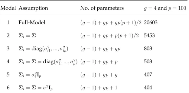
A commonly used way to reduce the number of parameters in a Guassian model is to impose constraints based on assumptions on the parameters of the model. This method can be illustrated by considering an example similar to the constrained Gaussian model given by Bouveyron and Brunet-Saumard (2014). Suppose an unconstrained Gaussian model (the full model) that highly parame-terized and contains 20603 parameters when there areg = 4groups andp= 100
variables. One possible constraint for reducing the number of parameters is to assume that all groups have the same covariance matrix, i.e. Σi = Σ,∀i, i =
assume that the variables are conditionally independent. This assumption im-plies that each covariance matrix is diagonal, i.e. Σi =diag(σi21, ..., σ2ip), whereσ2il
is variance of thelthvariable in theithgroup. In this case, where groups have the
same covariance matrix in addition to the independence assumption, the com-mon covariance matrix will be estimated as, Σ = diag(σ2
1, ..., σp2), where σ2l is
variance of thelthvariable in each group. Two other constraints are based on the
assumption that the covariance matrices are proportional to an identity matrix. They are: when the covariance matrix is spherical in each groupΣi = σi2Ip, and
when it is assumed that the covariance matrices are equal and spherical such that
Σi = Σ =σ2Ip, fori= 1,2..., gandσ2 ∈R.
For comparison, Table3.1lists the most commonly used model assumptions that can be obtained from a Gaussian mixture model withg groups andp vari-ables. The number of parameters can be decomposed into the number of param-eters for the proportions(g−1), for the meansgp, and for the covariance matrices (last term).
We can see that the full-model is a highly parameterized model. In contrast, the
5th and the 6th models are very parsimonious models (Bouveyron and
Brunet-Saumard, 2014). These models, however, work under the strong assumption of independence of variables which may be unrealistic in many discrimination problems. The second model requires estimation of an intermediate number of parameters, in this case 5453. This model is known to be an efficient model in practical classification problems. Furthermore, this model is commonly used when the normality assumption does not hold.
CHAPTER3. REVIEW OF DISCRIMINANT ANALYSIS IN HIGH-DIMENSIONS 37
Table 3.1: Number of parameters to estimate for constrained Gaussian models
Model Assumption No. of parameters g = 4andp= 100
1 Full-Model (g−1) +gp+gp(p+ 1)/2 20603 2 Σi =Σ (g−1) +gp+p(p+ 1)/2 5453 3 Σi =diag(σ2i1, ..., σip2) (g−1) +gp+gp 803 4 Σi =Σ=diag(σ21, ..., σ2p) (g−1) +gp+p 503 5 Σi =σ2iIp (g−1) +gp+g 407 6 Σi =Σ=σ2Ip (g−1) +gp+ 1 404
3.2
Regularization methods
In this section methods that mainly focus on estimating the within-class co-variance matrix using various regularization methods will be briefly reviewed. In general, methods of regularizing the within-class covariance matrix can be cat-egorized into two main groups. The first group of methods make an independent assumption that force the within-class covariance matrix to be diagonal. The sec-ond group of methods allow dependence and use various techniques to estimate the full covariance matrix (Clemmensen,2013).
3.2.1
Independence assumption
Because of the high dimensionpand small sample sizen, which are often re-ferred to aslargepsmalln, estimators of the sample mean and covariance matrix are usually unstable (Wang et al., 2013). Bickel and Levina (2004) have shown that Fisher’s LDA is no better than random guessing when p/n −→ ∞. From
the existing literature it is possible to classify the independence rules into two classes (Wang et al., 2013). The first and natural method is to ignore the depen-dence among the variables, which leads to the so called Naive Bayes Classifier. Some methods that assume independence are given in Tibshirani et al. (2003),
Tibshirani et al.(2002), andDudoit et al.(2002). These methods will be reviewed here briefly, together with a method that involves individual analysis (Fan and Fan,2008).
3.2.1.1 Nearest shrunken centroids (NSC)
Tibshirani et al.(2003) proposed a method for class prediction in high
dimen-sional microarray studies based on an enhancement of the nearest prototype clas-sifier. This method uses ’shrunken’ centroids as prototypes for each class where class centroids are shrunk toward the overall centroid.
In this approach, the covariance matrix is estimated as the diagonal of the full covariance estimateΣˆN SC =diag( ˆΣ) = diag(s21, s22, ..., s2p), wheres2l (l = 1,2, ..., p)
is variance of thelth variable. Consequently, the group means are shrunk using soft thresholding shrinkage. The absolute value of eachΣˆ−1N SCµˆiis reduced by an
amount∆and is set to zero if the result is less than zero. That is:
ˆ
Σ−1N SCµˆi∗ =sign( ˆΣ−1N SCµˆi)(|Σˆ−1N SCµˆi| −∆)+ (3.1)
where the subscript ’plus’ means the positive part (t+ =tift > 0). If the
shrink-age parameter is very large, many of the components (genes) will be eliminated. Hence,∆tunes the degree of sparsity. In particular, if∆causesΣˆ−1N SCµˆito shrink
to zero for all groups i, then the mean for variable l ,i.e.,X¯l, is the same for all
com-CHAPTER3. REVIEW OF DISCRIMINANT ANALYSIS IN HIGH-DIMENSIONS 39
putation. ∆is chosen by cross-validation. Similar methods can also be seen in
Dudoit et al.(2002) andTibshirani et al.(2002).
3.2.1.2 Independence rule (IR)
Bickel and Levina (2004) proposed an independence rule where the covari-ance matrix is estimated by the diagonal of the covaricovari-ance matrix. They ex-plained that the ’Naive Bayes’ classifier which assumes independence among variables greatly outperforms the Fisher LDA rule under certain conditions of the number of variables grows faster than the number of observations. They con-sidered the problem of discriminating between two groups withp-variate normal distributionsNp(µ1,Σ)and Np(µ2,Σ). A new observationxis to be assigned to
one of these two groups. Ifµ1,µ2, andΣare known, then the optimal classifier is
the Bayes Rule, expressed through the group indicator function1as:
δ(x) =1{log f1(x) f2(x) >0}=1(µTdΣ−1(x−µ)>0) (3.2)
where the prior probabilities are assumed to be equal and µd = µ1 − µ2 and µ= µ1+µ2
2 . Plugging all the parameter estimates directly into the Bayes Rule (2.4)
leads to the Fisher rule (FR):
δF(x) =1(ˆµTdΣˆ
−1
(x−µ)ˆ >0). (3.3)