Master’s Degree Programme in Computational and Systems Biology
Karolis Uziela
Making microarray and RNA-seq gene
expression data comparable
Master’s Thesis Espoo, June 30, 2012
Supervisors: Professor Juho Rousu, Aalto University
Professor Erik Aurell, KTH Royal Institute of Technology Instructor: Antti Honkela D.Sc. (Tech.)
Master’s Degree Programme in Computational and Systems Biology
ABSTRACT OF MASTER’S THESIS
Author: Karolis Uziela
Title:
Making microarray and RNA-seq gene expression data comparable
Date: June 30, 2012 Pages: vi + 61
Professorship: Information and Computer Science Code: T-61
Supervisors: Professor Juho Rousu Professor Erik Aurell
Instructor: Antti Honkela D.Sc. (Tech.)
Measuring gene expression levels in the cell is an important tool in biomedical sciences. It can be used in new drug development, disease diagnostics and many other areas. Currently, two most popular platforms for measuring gene expression are microarrays and RNA-sequencing (RNA-seq). Making the gene expression results more comparable between these two platforms is an important topic which has not yet been investigated enough.
In this thesis, we present a novel method, called PREBS, that addresses this issue. Our method adjusts RNA-seq data computational processing in a way that makes the resulting gene expression measures more similar to microarray-based gene expression measures. We compare our method against two other RNA-seq processing methods, RPKM and MMSEQ, and evaluate each method’s agreement with microarrays by calculating correlations between the platforms. We show that our method reaches the highest level of agreement among all of the methods in absolute expression scale and has a similar level of agreement as the other methods in differential expression scale.
Additionally, this thesis provides some background on gene expression, its mea-surement and computational analysis of gene expression data. Moreover, it gives a brief literature review on the past microarray–RNA-seq comparisons.
Keywords: Microarray, RNA-seq, gene expression, bioinformatics
Language: English
I would like to thank all of my friends and family for supporting me during the difficult time of writing the thesis. Moreover, I would like to thank my supervisors Prof. Juho Rousu and Prof. Erik Aurell, and especially my instructor Dr Antti Honkela for useful advice and comments regarding the thesis. Last but not least, I would like to thank my friends Andrew Keating and Maia Malonzo for keeping me a company during the lunch and coffee breaks.
Espoo, June 30, 2012 Karolis Uziela
CDF Chip Description File
DCPM Average depth of coverage per million reads
cDNA Complementary DNA
DNA Deoxyribonucleic acid
FDR False Discovery Rate
FPKM Fragments Per Kilobase of exon per Million fragments mapped
HIV Human Immunodeficiency Virus
LIMMA Linear Models for Microarray Data
Log2FC Log2 Fold Change
miRNA MicroRNA
MM probe Mismatch probe
MPSS Massively Parallel Signature Sequencing
mRNA Messenger RNA
PCR Polymerase chain reaction
PM probe Perfect match probe
PREBS Probe Region Expression Based on Sequencing qPCR (qRT-PCR) Quantitative real time PCR
RMA Robust Multichip Average
RNA Ribonucleic acid
RNA-seq RNA-sequencing
RPKM Reads Per Kilobase of exon per Million mapped reads
rRNA Ribosomal RNA
SAGE Serial Analysis of Gene Expression
siRNA Small interfering RNA
SNP Single-nucleotide polymorphism
TAR Transcriptionally Active Region
tRNA Transfer RNA
Abstract ii
Acknowledgments iii
Abbreviations and acronyms iv
1 Introduction 1
1.1 Problem setting . . . 1
1.2 Structure of the thesis . . . 2
2 Gene expression and its measurement 3 2.1 Biology of gene expression . . . 3
2.2 Gene expression measurement and data analysis . . . 5
2.2.1 Gene expression measurement methods . . . 5
2.2.2 Analysis of gene expression measurement data . . . 6
2.3 Microarrays . . . 7
2.3.1 Technical principles of microarray technology . . . 8
2.3.2 Computational analysis of microarray data . . . 10
2.4 RNA-sequencing . . . 12
2.4.1 Technical principles of RNA-seq technology . . . 12
2.4.2 Computational analysis of RNA-seq data . . . 14
3 Inter-platform gene expression data comparisons 16 3.1 Microarray–RNA-seq comparisons . . . 17
3.2 Methods that combine or visualize inter-platform data . . . . 21
4 Methods 23 4.1 Basic idea of the method . . . 23
4.2 Expression level inference . . . 25
4.3 Tools used for implementation . . . 26
5 Results 28
5.1 Data sets . . . 28
5.2 Absolute expression comparison . . . 29
5.3 Differential expression comparison . . . 35
5.4 Cross-platform differential expression . . . 40
5.5 Manufacturer’s CDF . . . 45
5.6 Differential expression in microarray technical replicates . . . . 47
6 Conclusion 49 6.1 Summary . . . 49
Introduction
1.1
Problem setting
Gene expression is a fundamental process in the cell during which the DNA is transcribed to the corresponding RNA and the RNA is translated to the corresponding protein. Gene expression levels can differ between different cells, tissues or points in time. Measuring gene expression has proven to be a very important tool in biomedical sciences, because it can be used for disease diagnostics, search for new drug targets and for analysis of diseases, such as cancer, Alzheimer’s disease, schizophrenia and HIV infection [1]. Therefore, gene expression measurement has been of great interest to scientists and many gene expression measurement methods have been developed.
Nowadays, two most popular gene expression measurement platforms are RNA-seq (RNA-sequencing) and microarrays. RNA-seq is a newer and more accurate technology [2, 3], but microarrays are still popular because they are cheaper and have a well established infrastructure [4]. On the other hand, it is predicted that in the future RNA-seq might fully replace microarrays [5]. This is also supported by Table 1.1 which shows that the number of RNA-seq experiments is rapidly increasing while the number of microarray experiments is slowly decreasing. That shows that the scientists are increasingly turning towards the newer gene expression measurement technology. However, even if the RNA-seq technology fully replaces microarrays we will still want to use the existing microarray data as a reference. There is a huge number of microarray experiments available in gene expression databases, such as ArrayExpress [6] or GEO [7], and therefore it is important to be able to compare the newly conducted RNA-seq experiments with existing microarray data in a meaningful way.
In the past, there have been many experimental RNA-seq–microarray
2010 2011 2012 Microarray 5796 5196 4724
RNA-seq 147 256 564
Table 1.1: Number of microarray and RNA-seq experiments in ArrayEx-press [6] database in the last three years. Data for the year 2012 is extrapo-lated based on the date when the query was made (June 25, 2012).
comparisons (they will be reviewed in Chapter 3). However, none of these comparisons tried to make RNA-seq and microarray data more similar, or, in other words, more comparable, by adjusting the computational processing of the data. In this thesis, we describe a method called PREBS that processes RNA-seq data in a way that the results become more similar to the microar-ray gene expression results. We evaluate our method by calculating gene expression correlations with microarrays and compare it against two other RNA-seq processing methods—RPKM [8] and MMSEQ [9]. We show that our method reaches the highest level of agreement with microarrays in abso-lute expression scale and a similar level of agreement as the other methods in differential expression scale.
1.2
Structure of the thesis
The thesis is organized as follows. In Chapter 2, we provide the background on gene expression, its measurement tools and analysis of the data. Two gene expression measurement tools, microarray and RNA-seq, are described in more detail.
In Chapter 3, we review past studies which were comparing or trying to combine/visualize inter-platform gene expression data. This review helps to get an understanding of the related work that has already been done.
In Chapter 4, we introduce our method and explain how it works. Addi-tionally, we list all of the tools that were used for the implementation.
In Chapter 5, we compare our method against two other RNA-seq pro-cessing methods: RPKM and MMSEQ. We demonstrate that our method agrees better with microarrays than the other two methods.
Finally, Chapter 6 concludes our work. Section 6.1 summarizes the work and Section 6.2 discusses the results and gives suggestions about possible future work.
Gene expression and its
measurement
In this chapter, we will review the necessary background that will be re-quired to understand the rest of the thesis. In Section 2.1, we will explain biological background of gene expression and, in Section 2.2, we will give a brief overview of its measurement methods and data analysis. Additionally, in Sections 2.3 and 2.4, we will look at the two currently most popular gene expression measurement tools, microarrays and RNA-seq, in more detail.
2.1
Biology of gene expression
All of the genetic information of the cell is encoded into DNA, a long double-stranded helical molecule composed of nucleotides. These nucleotides differ among themselves because of their side chains which are also calledbases. In DNA there are four different bases: adenine (A), guanine (G), cytosine (C) and thymine (T). The sequence of these four bases determines the genetic information encoded into DNA.
In order to make use of the genetic information, DNA first has to be transcribed to RNA. RNA chemical structure is very similar to DNA, except that instead of thymine (T) base it has uracil (U) base. RNA can sometimes be the final gene product, as it is in case of tRNA, rRNA, miRNA or siRNA. However, most common type of RNA is mRNA (messenger RNA) that is translated to proteins, molecules which are responsible for the most of the functions of the cell. The whole process of transcribing the DNA to the RNA and translating the RNA to the protein is called gene expression [10] (see Figure 2.1).
A single DNA strand can be viewed as a long string of letters A, C, G,
DNA
TranscriptionRNA
TranslationProtein
Figure 2.1: Basic scheme of gene expression. The DNA is first transcribed to RNA and then the RNA is translated into a proteinT, each of which stand for the base of a particular nucleotide. Not all of the DNA molecule is transcribed to RNA in a single transcription process, but only a small part of it. The substring of DNA which codes for a single RNA molecule is called a gene. During the process of transcription an enzyme called RNA polymerase reads the gene portion of the DNA and transcribes it to an RNA with complementary sequence. That is, adenine in the DNA is replaced with uracil in an RNA, cytosine is replaced with guanine, guanine is replaced with cytosine and thymine is replaced with adenine.
Before the mRNA can be translated into the protein, it undergoes post-transcriptional modifications. During this phase, 5’ cap and 3’ poly-A tail are added to the mRNA which protect the mRNA from degradation. More-over, during splicing process the non-coding parts of mRNA, introns, are removed and coding parts, exons, are joined together. The exons can be of-ten joined in a number of alternative ways, giving rise to different versions of the same gene—gene isoforms. RNA splicing and other post-transcriptional modifications occur only in eukaryotes, but not prokaryotes.
Next, during the translation phase the mRNA is translated into a protein. A protein is also a long macro-molecule like DNA and RNA, except that its subunits are not nucleotides, but amino acids. In most of organisms proteins are composed of 20 types of amino acids. Some organisms might, however, include two additional types of amino acids: selenocysteine and pyrrolysine [11].
Every three nucleotides in the mRNA code for one amino acid in a protein. During the translation phase, every three nucleotides in the mRNA are read and corresponding amino acid molecule is added to the protein chain which is being synthesized. After the whole protein is synthesized, it undergoes some more post-processing steps and folds into the correct shape. Then, it is transported to the appropriate place in the cell and can perform its function. Gene expression does not happen for all of the genes at the same time. If a gene is expressed at a particular point of time it is said to be active, otherwise, it is said to be passive. The rate of gene expression can also be different for different genes. If a lot of gene product is produced for a gene, the gene is said to have a high expression level, if only a little product is produced, the gene is said to have a low expression level.
2.2
Gene expression measurement and data
analysis
In this section, we will review the available tools for gene expression mea-surement. Moreover, we will provide an outline of the basic steps in gene expression analysis.
2.2.1
Gene expression measurement methods
Gene expression is defined as the conversion of genetic information into the actual protein [10]. Therefore, intuitively, gene expression level can be thought of as the amount of the corresponding protein present in the cell. There are some tools, such as Western Blot [12], which measure protein ex-pression levels in the cell. However, mRNA quantification is technically an easier task and it can be used as an approximation of the final gene product— protein [13]. So for the purposes of this thesis we will define gene expression level as the mRNA level and use these two terms interchangeably as it is also done by other scientists [13].
There is a variety of technologies available for quantifying mRNA lev-els in a cell. These technologies can be divided into two broad categories: hybridization-based and sequencing-based. The difference between the two is that hybridization-based technologies (Northern blot [14], qPCR [15], mi-croarrays [16]) use hybridization probes—short sequences which are comple-mentary to some part of expressed gene sequence. Designing these probes requires prior knowledge about the transcriptome which is being analyzed. On the other hand, sequencing-based technologies (RNA-seq [17], SAGE [18], MPSS [19]) do not use probes for gene expression analysis. There, the prin-ciple is to sequence the whole transcriptome and to determine the amount of reads which originate from each of the gene regions and, in this way, to evaluate gene expression levels.
Gene expression measurement technologies can also be divided into low-throughput and high-low-throughput categories. Low-low-throughput technologies can be used to analyze only from one up to several genes in the same exper-iment. On the other hand, high-throughput technologies allow us to analyze whole transcriptome—thousands of genes in the same experiment. All of the mentioned sequencing-based technologies and one hybridization-based tech-nology (microarrays) fall into the high-throughput category, while the rest of the hybridization-based technologies (Northern blot, qPCR) fall into the low-throughput category.
huge amount of genes that they can interrogate in one experiment. Mi-croarrays used to be a dominant high-throughput gene expression measure-ment platform, but nowadays RNA-seq is taking over its place [5]. Other sequencing-based high-throughput technologies (SAGE, MPSS) can be con-sidered as older variants of RNA-seq and are rarely used any more.
2.2.2
Analysis of gene expression measurement data
Gene expression data are often visualized as a gene expression matrix, a table where rows represent different genes, columns represent different sample conditions and each value represents the gene expression of a specific gene under a specific condition. Sample conditions can correspond to a number of different things, for example, different tissues, different disease states or samples taken at different points of time. Genes in the table can represent either all or some subset of the genes from the organism being analyzed [13, 20].
Gene expression measures inside the matrix can be either in an absolute or a relative scale. In case of an absolute scale, the values in gene expression matrix represent an absolute gene expression measurement in some abstract units, while, in case of a relative scale, the values are gene expression ratios between two conditions. The ratios of gene expression are often more inter-esting to the scientists, because they show how much expression values differ between two conditions of an experiment. Genes which have statistically sig-nificant changes in expression are called differentially expressed genes [20].
A natural way to analyze gene expression matrix is either to compare rows or columns of the table. However, for a comparison we need to decide what similarity measure to use. Most commonly used similarity measures are Euclidean distance, Pearson correlation, Spearman correlation or mutual information. It is difficult to tell which similarity measure is the best to use and it can often depend on the type of experiment being conducted [13].
After choosing the similarity measure, there are two major ways to an-alyze the data: supervised learning and unsupervised learning. In case of supervised learning, the data rows or columns have to be associated with some known features. It could be, for example, gene functions for rows or disease states for columns. Then some sort of a classifier is built which is trained to predict these features. Some of the popular methods used in gene expression analysis for classification are linear discriminants, decision trees and Support Vector Machines. After building a classifier, it can be used to predict features for new data. Moreover, if a classifier is built with some rel-atively simple classification rules, it can also be used to infer the underlying biological mechanisms of the system [13].
Affymetrix Agilent Illumina Nimblegen Other Count 13832 3091 1715 800 7456
Table 2.1: Number of experiments in ArrayExpress database for each mi-croarray platform as of June 20, 2012
In unsupervised learning the aim is to group objects (genes or samples) with similar properties. Some of the popular clustering methods that are used are K-means, Hierarchical clustering and Self-organizing maps. These methods can be, for example, used to cluster the genes with similar expres-sion patterns in order to identify common transcription-control mechanisms. Clustering genes can also help to infer function for an unknown gene, because genes with similar expression patterns tend to share a similar function [13]. Furthermore, clustering of the samples, can, for example, be used to infer new sub-classes of tumors as it was done by Alizadeh et al. [21].
2.3
Microarrays
Microarrays have evolved from Southern Blotting, a technique which is used to identify a specific DNA sequence in DNA samples [22]. The first studies that involved microarrays were published in 1980s, but the real microarrays take-off began with a publication by Fodor et al. [23] from Affymax, a com-pany which later changed its name to Affymetrix and became the market leader for microarray technology. Fodor et al. described protein and nu-cleotide microarrays, their uses and design principles. Since then microarray technology became more and more popular and, in the beginning of 21st century, one could hardly find a modern biology or genetics journal which does not mention microarrays [16].
Nowadays, besides Affymetrix, the other popular platforms include Ag-ilent, Illumina and Nimblegen. In order to see what are the approximate market shares of the commercial microarray platforms in academic use, we queried each platform name on ArrayExpress [6] database. The results are displayed in Table 2.1. As the results show, Affymetrix is by far the most popular platform and it takes up more than 50% of the whole market. There-fore, in this thesis most emphasis will be put on the Affymetrix microarray technology description and data analysis.
In this section we will shortly describe the basic principles of microarrays and review different types of technology. In addition, we will give a brief introduction to computational analysis of microarray data.
2.3.1
Technical principles of microarray technology
Typically, a microarray consists of a large number microscopic DNA spots attached to a solid surface. Each of the spots contains many short DNA sequences called probes. All of the probes inside one spot have the same sequence. Also, all of the probe sequences are complementary to a part of the gene from an organism which is being analyzed. Different spots on the microarray correspond to different genes, so the more spots a microarray has, the more genes can be interrogated at the same time.
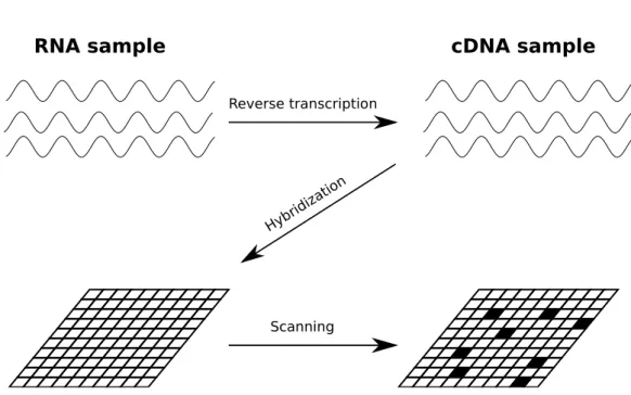
In order to conduct a microarray experiment, one has to extract RNA from the cell and reverse transcribe it to cDNA (complementary DNA) (see Figure 2.2). In this step, thereverse transcriptase enzyme synthesizes a DNA molecule which has complementary sequence to the given RNA molecule. The reason of doing this is that an RNA molecule is less stable than a DNA molecule, so the molecule conversion helps to improve the stability without losing the genetic information.
In the next step, the cDNA sample has to be fluorescently labeled (other labeling methods are also possible). The labeled sample is poured on top of the microarray and the cDNA molecules hybridize onto the microarray probes based on their complementarity. The spots where cDNA molecules have attached can be identified because of the fluorescent dye. The stronger the signal (fluorescence intensity) is for a spot, the higher is the gene expression level for the gene to which that spot corresponds.
The above described principles hold only for what is called gene expres-sion microarrays [1]. The purpose of these microarrays is to measure gene expression (mRNA) levels inside a cell. There are many other kinds of mi-croarrays that can be used for different purposes. For example, antibody microarrays [24] can be used to measure protein expression levels, SNP mi-croarrays [25] can be used to detect Single Nucleotide Polymorphisms, tiling microarrays [26] can be used for ChIP-on-chip [27] studies.
Tiling microarrays can also be used for gene expression profiling like gene expression microarrays, but there are some important differences between the technologies. The main difference is that the probe sequences for tiling arrays are not selected from the genes being investigated, but instead they are taken at regular intervals from the whole genome. In this way, there is a possibility for new genes to be identified in the genome places which were previously thought to be non-transcribed. However, tiling microarrays are more expensive and are not as commonly used for gene expression profiling as gene expression microarrays. In this thesis, we will concentrate on analyzing only gene expression microarrays.
RNA sample cDNA sample Reverse transcription Hybr idiza tion Scanning
Figure 2.2: Microarray workflow scheme. First, RNA sample is reverse tran-scribed to cDNA. Then cDNA sample is poured on top of the microarray to allow probes with complementary sequence to hybridize. Finally, the microarray is analyzed by a special machine to determine fluorescent dye intensities (scanning)
spotted microarrays andoligonucleotide microarrays [1]. The main difference between the two is that in spotted microarrays the probes usually consist of long cDNA molecules (several hundreds of base pairs) which are prepared beforehand and are printed on the microarray by a robotic arm. In oligonu-cleotide microarrays, the probes are short oligonuoligonu-cleotides (typically, 25-100 bp long) which are synthesized directly on the microarray plate.
Another important difference lies in the target preparation. In oligonu-cleotide microarrays, the target is labeled by one fluorescent dye and, in order to identify the differentially expressed genes, the signal intensity is compared between two microarrays. However, the probe preparation procedure for spotted microarrays is not as accurate as for oligonucleotide microarrays and comparison between two separate microarrays would not be possible. There-fore, for spotted microarrays two target samples are labeled by two different fluorescent dyes (typically Cy3 and Cy5) and the differential gene expression is identified by the ratio of two different signals on a single microarray [1].
Spotted microarrays are often termedin-house microarrays, because they are prepared in individual labs [28]. For this type of microarrays, the re-searchers conducting an experiment can decide which genes they want to
interrogate and design a microarray suiting their needs. On the other hand, oligonucleotide microarrays are usually called commercial microarrays, be-cause they are mass-produced by industrial companies. These microarrays usually aim to interrogate all known genes in the target organism transcrip-tome. Spotted microarrays were more popular in the past, because they were cheaper and more customizable. Nowadays, however, spotted microarrays are rarely used any more, because oligonucleotide microarrays have become more affordable and provide more accurate results [16]. Also, the design of oligonucleotide microarrays became customizable via availability of custom oligonucleotide arrays [29]. In this thesis we will analyze only oligonucleotide microarrays.
2.3.2
Computational analysis of microarray data
Computational analysis of microarray data largely depends on the type of microarray platform being used. Since, as we mentioned before, Affymetrix is, at the moment, the dominant microarray platform, we will discuss the data analysis only for this platform.
Affymetrix microarrays consist of many 25 nucleotides long probes at-tached to a solid surface [30]. There are of two types of probes: perfect match (PM) and mismatch (MM). Perfect match probes are perfectly complemen-tary to some part of a target gene which they are interrogating. Mismatch probes, on the other hand, have the same sequence as perfect match probes, but the middle nucleotide (13th) is changed. Some microarray methods use mismatch probes to account for non-specific probe binding while other meth-ods simply ignore the intensity values of the mismatch probe hybridization.
The probes are grouped into probe sets by the manufacturer. Typically, a probe set contains 15–20 PM/MM probe pairs and it interrogates one tar-get gene. The information about the probe sets is available in so called
Chip Description Files (CDFs). However, transcriptome annotations change over time and some of the probes might appear to be mapping not to one, but to several genes or do not correspond to any genes at all. The man-ufacturer’s CDFs are rarely updated, therefore, many people prefer to use custom CDFs [31] which account for the latest changes in the transcriptome annotation. In these files, probes that do not map uniquely to a single gene are filtered out and the rest of them are regrouped to new probe sets each of which corresponds to a single gene in the latest transcriptome annotation.
In general, probes belonging to one probe set can give different hybridiza-tion intensity values in an experiment. Furthermore, the microarray exper-iments are often done with replicates—the same experiment is done several times to reduce variability. The first step in microarray computational
anal-ysis is to summarize probe intensities from all probe sets and all microarray replicates to get a single gene expression measure for each gene. Many algo-rithms have been developed for this procedure, most popular of them being RMA [30] and MAS5 [32]. RMA is open source software, while MAS5 is Affymetrix proprietary method.
Both of these algorithms use some background-correction, normalization and summarization procedures. During the background-correction phase the probe intensity values are adjusted to account for technical noise, then, dur-ing normalization phase, probe intensity values are normalized to be compa-rable across different microarrays and, finally, during summarization phase, probe intensities are converted to gene expression measures.
The main difference between RMA and MAS5 is that RMA uses only values from PM probes while MAS5 uses values from both PM and MM probes. In MAS5 algorithm, MM values are subtracted from PM values to account for non-specific binding while RMA algorithm simply ignores MM values. Another important difference is that MAS5 normalizes every mi-croarray independently while RMA normalizes all mimi-croarrays at the same time. Nowadays, RMA algorithm is more often used than MAS5, therefore, for the rest of the thesis we will restrict ourselves only on analyzing results with RMA.
Further analysis of microarray data often include identification of differ-entially expressed genes. There are many tools for this task, but one of the most popular of such tools is LIMMA [33]. Among other results, LIMMA outputs log2 fold change values. These values show how much gene expres-sion has changed from one condition to another. They are determined, by calculating the ratio of absolute gene expression measures in the two samples and then taking base 2 logarithm of the ratio. In addition to that, LIMMA uses moderated t-test to calculate p-values. A p-value is a probability, as-suming that the null hypothesis is true, to obtain a statistic value at least as inconsistent with the null hypothesis as the one observed [34]. In our case, the null hypothesis says that the gene is not differentially expressed, there-fore,p-value measures statistical significance of differentially expressed genes. LIMMA also outputs adjusted p-values which are more commonly known as
False Discovery Rate (FDR) values. False Discovery Rate is a technique which is used to account for multiple testing problem and it denotes the percentage of false positives among the significant hypotheses [35].
2.4
RNA-sequencing
For over a decade, microarrays were the dominant platform in the high-throughput analysis of gene expression [36]. Sequencing-based methods, such as SAGE or MPSS, used to be the major alternative methods. One of the advantages of these methods is that they provided precise digital gene expression measures instead of analog expression measures provided by mi-croarrays1. These methods, however, were based on a conventional Sanger sequencing, and they were not as efficient as later developed methods based on next-generation sequencing [17].
There are several different technologies which correspond to the next-generation sequencing, but all of them have one thing in common— sequencing is done via massive parallelization. At the moment, three most popular next-generation sequencing technologies are Roche/454, Illumina and AB SOLiD [36]. Their ability to sequence transcriptome cost-effectively and in a high depth gave birth to a new technology for gene expression measurement—RNA-sequencing (RNA-seq) [17].
In this section, we review the basic principles of the next-generation se-quencing technologies and the steps needed to take in order to conduct an RNA-seq experiment. Also, we give a brief overview of the computational methods involved in RNA-seq data analysis.
2.4.1
Technical principles of RNA-seq technology
The first key step in the next-generation sequencing is sample preparation. The procedure varies from technology to technology, but the basic princi-ples remain the same: coding RNA (mRNA) has to be separated from the rest of the sample, reverse transcribed, fragmented and amplified [17]. For separation purposes, poly-A tail of the mRNA is often targeted by poly-T oligonucleotides attached to a given substrate. Next, the mRNA is reverse-transcribed to cDNA and fragmented into sizes required by the specific pro-tocol. The amplification can be carried out in a few different ways: 454 and SOLiD use emulsion PCR [39] while Illumina uses bridge amplification [40]. The end result for any sample preparation is the same: a number of short single-stranded cDNA molecules separated into clusters or microscopic wells on a plate and ready to be sequenced [41].
The next-generation sequencing technology which was developed the first 1Some of the studies claim that another advantage of SAGE is the ability to detect
novel transcripts [37, 38]. However, one of the studies [8] explicitly state that SAGE is not able to detect novel transcripts which is a little bit confusing.
is Roche/454 [41, 42]. This sequencing method is based on sequencing by synthesis methodology. Sequencing is done by synthesizing a complemen-tary DNA strand for each of the oligonucleotides on a plate. During the sequencing process, all four types of nucleotides (A, G, C, T) are added to the sequencing reaction sequentially, one at a time. If some particular DNA strand can be extended by the added nucleotide based on the complemen-tarity principle, a DNA polymerase adds that nucleotide to the DNA strand being synthesized. This causes a special reaction where an inorganic phos-phate ion is released and a flash of light is observed. In case of repetitive sequence, several nucleotides are added during one cycle and the intensity of the light being released becomes proportionally stronger. Light intensi-ties and positions on a plate are captured by a monitor. Unincorporated nucleotides are washed away and the sequencing reaction becomes ready for the next cycle. This reaction is repeated many times, until all of the oligonu-cleotide sequences are determined.
Illumina uses a similar approach as 454 which is also based on sequencing by synthesis [41, 40]. The main difference is that following Illumina tech-nology, all four types of nucleotides are added at the same time. Each of them, however, are labeled by a different fluorescent dye and have a termi-nating group which prevents the chain extension by more than one nucleotide. After each chain on a plate is extended by one nucleotide, unincorporated nucleotides are removed and the types of incorporated nucleotides are deter-mined by color imaging. Next, fluorescent dyes and terminating groups are removed and the sequencing reaction is ready for the next cycle. As it was in case of 454, the cycles are repeated until all of the sequences are determined. SOLiD system is based on a different methodology which is called se-quencing by ligation [41, 43]. First, a universal primer and 8-base long fluo-rescently labeled oligonucleotide probes are added to the reaction. Of these 8 bases only the first two are meaningful, the rest of them are degenerate, meaning that they can pair with any other base. The oligonucleotide probe binds to the DNA strand being sequenced and a DNA ligase enzyme links the oligonucleotide to the growing strand. The unlinked oligonucleotides are washed away and the fluorescent label is read by a scanner. Next, three trailing degenerate nucleotides are cleaved off and new oligonucleotides are added. This process continues until the new strand is fully synthesized. After this, the whole new strand is denaturated and the whole process is repeated with the only difference that a new primer is one nucleotide shorter than the previous one. As a result, new bases are read during the process. The whole reaction is repeated five times, to ensure that each nucleotide on the strand is interrogated twice. In this system, only 4 fluorescent colors are used to label 16 types of oligonucleotide probes, but this is sufficient, because the sequence
can be later inferred based on a set of logical rules, known as 4-color coding scheme [41].
After the sequencing is completed, the data has to be computationally analyzed. The exact type of analysis depends on what kind of experiment we want to conduct. In addition to gene expression profiling, RNA-seq data can be used for non-coding RNA discovery and detection, transcript rearrange-ment discovery or single-nucleotide variation profiling [44]. We, however, will focus only on RNA-seq applications for the gene expression profiling.
2.4.2
Computational analysis of RNA-seq data
In the computational analysis description we will assume that the genome of the species being investigated is known. In that case, the first step is to map the sequencing reads to the reference genome in order to know where they have originated from. This process is not complicated for individual reads, but the problem arises because of the huge amount of reads that need to be mapped. Conventional alignment programs such as BLAST or BLAT would simply be too slow for this task [45]. Hence, new alignment tools have been developed which are aimed at aligning a large amount of short read data. One of the most popular tools used for this task is Bowtie [46], a program which aligns the short reads in a very fast and memory efficient way.
Another problem for read mapping might be caused because of repetitive regions in a genome. Reads originating from these regions usually cannot be mapped unambiguously. In higher eukaryotic organisms, these regions constitute almost 50% of the genome [45], so discarding all of those reads would result in a substantial loss of the data. Therefore, many studies use
pair-ended reads. The idea is that a DNA fragment is sequenced from both of its ends giving rise to two reads with approximately known gap length between them. In this way, aligning one of the paired reads could help to align the other one unambiguously. Nowadays, pair-ended reads are supported by most of the sequencing platforms and alignment tools [45].
Yet another problem is caused by reads originating from the locations of splice junctions. These reads cannot be straightforwardly mapped to the original genome, because the read sequence is split into two parts and sepa-rated by an intron sequence in the original genome. Some of the alignment programs take into consideration the existing transcriptome annotations or even try to find novel splice junctions in order to map such reads. One of the most popular program among these is TopHat [47]. Original Bowtie soft-ware was not able to deal with such reads, but the problem is addressed in Bowtie 2 [48], a new version of the tool which is currently under the devel-opment.
After the reads are mapped, the gene expression levels can be inferred simply by counting how many mapped reads fall into the regions of known genes [8]. In the fragmentation step, longer genes get more fragments for sequencing, therefore, the counts for each gene have to be normalized by gene lengths. Moreover, these counts have to be normalized by the total number of mapped reads for a sample, because some samples might have more mapped reads than the others which would result in a sample bias. A popular gene expression measure which follows these principles is called RPKM (Reads Per Kilobase of exon model per Million mapped reads) [8]. It normalizes read counts by gene lengths in kilobases and by millions of mapped reads for a sample.
More advanced methods, such as Cufflinks [49], MMSEQ [9] or Bit-Seq [50], measure gene expression levels not on the gene level, but on the isoform level. Since gene isoform sequences are very similar, many reads can often be mapped to several gene isoforms. If we discarded all of those reads, it would be difficult to estimate the expression levels for separate isoforms. Therefore, a statistical model has to be created which aims to tell how many of these reads originate from each of the isoform. Parameters of the model are usually adjusted by looking at the reads which map to the distinct parts of the isoforms. Having isoform level expressions, gene expressions can be derived by summing up all of the isoform expressions belonging to a single gene.
As it was in the case of microarrays, the downstream analysis often include identification of differentially expressed genes. One of the most popular tools used for this task are DESeq [51] and edgeR [52]. Similarly to microarray differential expression analysis tool LIMMA, DESeq and edgeR calculate log2 fold change values,p-values and FDR values. However, unlike LIMMA, for calculating p-values these tools use a statistical test that is based on a negative binomial distribution.
Inter-platform gene expression
data comparisons
RNA-seq technology offers many advantages over conventional microarrays, such as a low background signal, a possibility to detect novel transcripts and an increased dynamic range of measurements [2, 17]. Therefore, RNA-seq has already become a popular alternative to microarrays and it is likely that in the future it will fully replace microarrays [5]. However, there are some im-portant practical considerations which favor microarrays: lower cost, known biases and well-established experimental pipelines [4]. Thus, microarrays still remain a popular technology for dealing with gene expression data.
Naturally, there is a need to compare microarray experiments against RNA-seq experiments. Previously, such comparisons usually aimed at eval-uating the reliability of RNA-seq technology [2, 3], but in the future such comparisons might more often be used in order to retrieve similar microarray– RNA-seq experiment pairs and get more insight on a particular study. These comparisons will still be relevant even if microarrays are fully replaced by RNA-seq, because there are big databases of microarray experiments avail-able [6, 7] and they could be used as a reference.
In order to make these comparisons more effective, we have to find a way, how to convert the measurements of microarrays and RNA-seq or how to change the processing of their raw data in order to make these measurments more similar or more ”comparable”. However, to the best of our knowledge, there are no past studies which would had been aiming at doing that. On the other hand, there were previous studies that are 1) comparing the platforms in order to estimate their accuracy, 2) performing the same experiment on two platforms in order to validate results, 3) visualizing data from the two platforms 4) combining the data from two platforms in order to extract some new information about the experiment. In this chapter, we will first present
the studies which were comparing the two platforms (1 and 2) and then we will give a short overview of the studies which were combining or visualizing data from the two platforms (3 and 4).
3.1
Microarray–RNA-seq comparisons
One of the earliest and most prominent microarray–RNA-seq comparisons was done by Marioniet al.[2]. This study evaluated RNA-seq technical repro-ducibility and compared the RNA-seq and microarray gene expression mea-surements. The RNA-seq platform used in the study was Illumina Genome Analyzer and the microarray platform was Affymetrix U133 Plus 2. RNA-seq and microarray experiments were done using the same samples taken from human kidney and liver. Sequencing was done in 2 runs, each of the runs was using 7 lanes where some of the lanes contained kidney samples while the other lanes contained liver samples. Microarray experiment was done with 3 technical replicates for each kidney and liver sample.
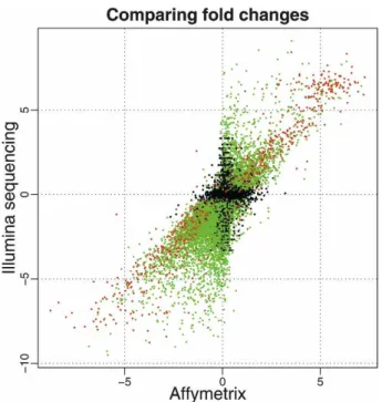
RNA-seq data was shown to be highly reproducible and the technical variance across the lanes was very small. In addition, RNA-seq gene expres-sion measures were found to agree with microarray gene expresexpres-sion measures rather well both on an absolute and differential gene expression scale. The Spearman correlation was 0.75 for kidney, 0.73 for liver and 0.73 for log2 fold changes between the two conditions (Fig. 3.1). 11493 genes were found dif-ferentially expressed at FDR of 0.1% according to RNA-seq and 8113 genes according to microarray technology. Among these, the majority (6534) were found to be differentially expressed according to both platforms. In order to find out which of the platforms gives more accurate results, they were compared against the third technology—qRT-PCR. The results of qRT-PCR were found to agree better with RNA-seq giving an indication that RNA-seq is a more sensitive method at detecting differentially expressed genes.
Another prominent study by Fuet al.[3] compared microarrays and RNA-seq with the third dataset coming from an independent source—proteomics. Sequencing platform used was Illumina’s Solexa Sequencer, microarray plat-form was Affymetrix Human Exon 1.0 ST and protein expression levels were measured by 2D LC-MS/MS system. Absolute gene expression measure-ments of a human brain sample were calculated for both platforms. The Pearson correlation between RNA-seq and microarray measurements was rea-sonably good: r = 0.67 for 8441 genes. For a subset of 520 genes RNA-seq and microarrays were compared against proteomics. The Pearson correla-tion was of a moderate level, but it was better for RNA-seq than microarrays (r = 0.36 for RNA-seq and r= 0.24 for microarrays). Hence, RNA-seq was
Figure 3.1: A comparison of log2 fold changes between Affymetrix and Illu-mina platforms by Marioni et al. [2]. Differentially expressed genes having more than 250 reads are colored red and genes having less than 250 reads are colored green. Reads that are not differentially expressed at FDR of 0.1% are colored black.
concluded to be a more precise method for an absolute gene expression level estimation.
A particularly interesting inter-platform comparison was done by Agar-wal et al. [53] comparing tiling arrays against Solexa/Illumina sequencing technology. Tiling arrays are the only type of microarrays which is able to detect novel transcripts. Therefore, RNA-seq and tiling arrays were com-pared not only by their gene expression measurements, but also by their ability to detect known transcriptionally active regions (TARs). The de-tected TARs were compared with a gold standard set—known transcriptome annotations. RNA-seq was found to be in a better agreement with known transcriptome annotations, hence, it was suggested that RNA-seq could be used to calibrate tiling arrays for detecting unknown transcripts.
An another interesting study was done by Bradfordet al.[54]. Expression measurements of human breast cell lines were compared between SOLiD sequencing platform and Affymetrix Human Exon 1.0 ST microarrays. The difference between this study and the previously mentioned studies is that in
this study, expression measures were compared not on a gene level, but on an exon level. The Pearson correlations were r = 0.55 for MCF-10a cell line and r = 0.53 for MCF-7 cell line. The log2 fold change correlation for the exons expressed in both conditions was r = 0.59.
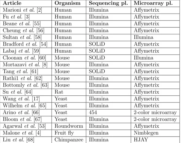
All of the above mentioned and some of the other microarray–RNA-seq comparisons are listed in Table 3.1. The list is not exhaustive, but includes most of the published comparisons up to this date. As we can see, most of the comparisons were done on human samples, but there were some comparisons on mouse, yeast and other organisms. Most of the studies compared Illumina sequencing platform against Affymetrix microarray platform, but there were some comparisons between other types of platforms, too. For many of the studies, the inter-platform comparison and evaluation of RNA-seq platform reliability was the major purpose, however, some of the studies were aimed at biology-related questions and the comparisons were done just as an additional validation of experimental results [55, 56].
Most of the studies calculated either absolute gene expression measure-ment or log2 fold change correlation between the two platforms. Both abso-lute gene expression and log2 fold change correlations varied between studies. For example, in Beaneet al.[55] log2fold change correlation between Illumina sequencing and Affymetrix HGU133A 2.0 microarray was only 0.16, while in Marioni et al. [2] it was 0.73. The correlation levels rarely depend on which type, Pearson or Spearman, correlation measurement is used. However, they depend a lot on the way experiment samples are prepared. If the exact same experiment samples are being used for both RNA-seq and microarray studies and the sample preparation protocol is very similar, the correlation between the two platforms is significantly better. For log2 fold change correlations there is an another important factor: the similarity of the two sample con-ditions. If the conditions are very similar, log2 fold change values are very small and the two platforms are not able to measure them precisely because of the noise. Therefore, in this case, the two platforms do not agree as well as in the case of where two sample conditions are very different. Finally, one should remember that the correlation significance largely depends on the number of points being correlated [57]. Therefore, in general, one could ex-pect a lower correlation coefficient if the correlation is calculated for a large number of genes and a higher correlation coefficient if it is calculated for a small number of genes.
In the past, there were also many studies which compared gene expres-sion measurements across different microarray platforms [28, 69, 70, 37]. In some of these studies, the correlation between different microarray platforms is even worse than the correlations between RNA-seq and microarray in the above mentioned studies. For example in Liu et al. [37], the absolute gene
Article Organism Sequencing pl. Microarray pl.
Marioni et al. [2] Human Illumina Affymetrix
Fuet al. [3] Human Illumina Affymetrix
Beaneet al. [55] Human Illumina Affymetrix
Cheunget al. [56] Human Illumina Affymetrix
Sultanet al. [58] Human Illumina Illumina
Bradfordet al. [54] Human SOLiD Affymetrix
Labajet al. [59] Human SOLiD Affymetrix
Cloonan et al.[60] Mouse SOLiD Illumina
Mortazaviet al. [8] Mouse Illumina Affymetrix Tanget al. [61] Mouse SOLiD Affymetrix
Rathi1 et al. [62] Mouse Illumina Affymetrix
Bottomly et al. [63] Mouse Illumina Affymetrix Suet al. [64] Rat Illumina Affymetrix Wang et al.[17] Yeast Illumina Affymetrix
Wilhelm et al.[65] Yeast Illumina Affymetrix
Arino et al. [66] Yeast 454 2-color microarray
Bloom et al. [67] Yeast Illumina 2-color microarray Agarwal et al. [53] Roundworm Illumina Affymetrix
Malone et al. [4] Fruit fly Illumina Nimblegen Liuet al. [68] Chimpanzee Illumina HJAY
Table 3.1: Publications that compare RNA-seq – microarray gene expression data
expression measurement correlations between different microarray platforms ranged only from 0.42 to 0.60. This is an another indication that we can-not expect a perfect correlation between different platforms, especially given different sample preparation protocols. However, we can still look for the ways to reduce the gene expression measurement differences by computa-tional analysis and aim at increasing the inter-platform correlation as we will be doing in this thesis.
3.2
Methods that combine or visualize
inter-platform data
There have been a few studies which developed tools for combined microarray– RNA-seq gene expression data processing, visualization and statistical analy-sis [71–73]. The common feature of these tools is that they all support several different RNA-seq and microarray platforms, employ traditional gene expres-sion data processing algorithms and have a few different ways of visualizing the data.
Among these tools, probably the most universal and well-known tool is Mayday SeaSight [71] which is an extension of an older version of the tool Mayday [74, 75]. The main new feature of the extension is the ability to handle sequencing data, in addition to microarray data. As sequencing data input SeaSight takes a mapped reads file in SAM or BAM format while as microarray data input it takes raw output files from GenePix, Affymetrix, Agilent or ImaGene platforms. Alternatively, it can take generic tabular for-mat files as sequencing or microarray data input. SeaSight has a number of different possible data processing methods both for microarray (background correction, two-channel array normalization, inter-array normalization and summarization) and sequencing (RPKM, DCPM and locus-dependent func-tions). Also, the original Mayday software offers many plugins which can be used for data clustering, filtering, classification and for finding significantly differentially expressed genes. Finally, the data can be visualized in a num-ber of different ways: scatter plots, box plots, profile plots or enhanced heat maps.
Some of the past studies created methods that combine gene expression measurements from several microarray platforms in order to get some addi-tional information about the experiment [76, 77]. Warnat et al.[76] has used gene expression data from several different microarray platforms to classify the samples between three different diseases: prostate cancer, breast cancer and acute myeloid leukemia. The gene expression measurements were
trans-formed using either Median Rank Score or Quantile discretization algorithm in order to make them more comparable and then they were used as an input for Support-Vector-Machine-based classifier. In another study, Wang
et al. [77] used factor analysis to unify gene expression data from several microarray platforms. The factor analysis was performed either on gene ex-pression level or probe exex-pression level. The method accuracy was evaluated by comparing it to an independent dataset—gene expression measurements from SAGE platform.
To the best of our knowledge, so far there have not been any attempts to combine gene expression data from microarray and sequencing platforms or from two different sequencing platforms. There was one study which com-bined results from two RNA-seq experiments, but the study was concerned not with the gene expression measurements, but with the transcriptome an-notation [77]. The two experiment results were combined in order to identify more novel transcripts and splice sites. On the other hand, combination of RNA-seq and microarray gene expression results is possible in principle and might be done in the future. This could be another motivation to make RNA-seq and microarray gene expression measurements more comparable, as we are aiming in this thesis.
Methods
In this chapter, we present our method that aims to make microarray and RNA-seq gene expression data more comparable. Section 4.1 explains the main idea of our method, Section 4.2 gives the details about the statistical model which we used to infer expression levels and Section 4.3 provides the information about the tools used for implementation.
4.1
Basic idea of the method
One of the fundamental differences between microarrays and RNA-seq is that RNA-seq measures gene expression based on the whole gene sequence while microarrays rely only on the sub-portion of the gene where the microarray probe sequences are located. The idea of our method is to eliminate this difference, by calculating gene expression for RNA-seq using only the gene regions where probe sequences are located.
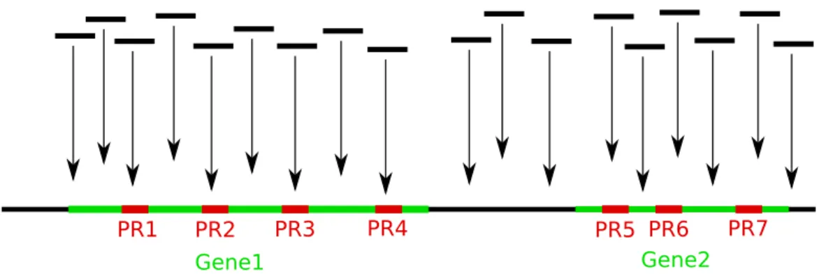
The basic idea of our method is illustrated in the Figure 4.1. Usually, in RNA-seq technology, gene expression is calculated based on the number of mapped reads overlapping with gene regions. We, on the other hand, counted the number of reads overlapping with probe regions. Probe region locations were retrieved from Custom CDF probe annotation files [31].
Based on the read counts we estimated probe region expressions using a probabilistic approach (more details on this step will be provided in Sec-tion 4.2). As a result, we got probe region expressions using the sequencing data. Each probe region expression has a corresponding probe expression in the microarray. Therefore, from this point we treated probe region ex-pressions the same way as probe exex-pressions are treated in microarray data analysis. That is, we applied one of the most popular algorithms for microar-ray data analysis—RMA.
PR1 PR2 PR3 PR4 PR5 PR6 PR7
Gene1 Gene2
Figure 4.1: Counting reads overlapping with probe regions. Gene1 and Gene2 denotes gene regions, while PR1-PR7 denotes probe regions inside the gene regions.
The RMA algorithm (which was also discussed in Section 2.3.2 of Chap-ter 2) consist of three steps: background-correction, normalization and sum-marization. During background-correction step, technical noise is removed, during normalization step, the expression values from different microarray replicates are normalized and, finally, during summarization step, probe-level expressions are converted to gene-level expressions. Since sequencing data contains very little technical noise [17], we skipped background-correction step and applied only the two latter steps of RMA.
We call our method PREBS—Probe Region Expression Based on Se-quencing. The basic pipeline for the whole method is depicted in Figure 4.2. In short, we count read overlaps with probe regions to get probe region ex-pressions and then we apply RMA to get gene exex-pressions. This type of sequencing data processing resembles microarray data processing and, as we will see later, the gene expression results which we get this way are more similar to microarray gene expression results.
Sequencing data
Count reads overlapping with probe regions
Probe region expressions
Apply RMA
Gene
expressions Figure 4.2: Basic pipeline to get gene expression measurements using PREBS method
4.2
Expression level inference
Counting the number of reads that overlap with regions of interest (probe regions or gene regions) is a stochastic process. As a result, there is a lot of uncertainty about the observed counts for these regions, especially, when the counts are small. In order to account for the uncertainty, we decided to use a probabilistic approach.
We use Bayesian inference [78] which is based on Bayes rule:
P(H|E) = P(E|H)·P(H)
P(E) ∝P(E|H)·P(H). (4.1) Bayes rule says that theposterior P(H|E) is equal to the likelihood P(E|H) times prior P(H) divided by the evidence P(E). We can often choose to ignore the normalizing factor (evidence) and then we get that the posterior is proportional to the likelihood times the prior. In our case, the evidence E
will be the number of mapped reads that overlap with the region of interest in a genome and the hypothesis H will be the distribution of those reads.
Each sampled read has two possibilities: either it overlaps with the re-gion of interest or it does not. Therefore, read sampling can be modeled as a Bernoulli process and the read distribution converges to a Poisson distri-bution as the number of reads approaches infinity [79]. The number of reads
k mapped to the region of interest depends on the Poisson distribution with a rate parameter λ and it can be modeled by
p(k|λ) = Poisson(k;λ) = λ ke−λ
k! , (4.2)
where λ parameter can be viewed as the gene expression level of the region of interest or, in other words, the rate by which reads are sampled from that region.
Equation (4.2) will be our likelihoodP(E|H). In order to select the prior
P(H), we have to select a distribution for λ parameter. In this case, the most convenient distribution for the prior is the Gamma distribution
p(λ) = Gamma(λ;α, β) = β α Γ(α)λ
α−1
e−βλ, (4.3)
because it is conjugate to the Poisson distribution. That means, if the like-lihood is a Poisson distribution and the prior is a Gamma distribution then the posterior P(H|E) will also be a Gamma distribution [80]. If we have a
single measurement of k, it can be shown that posterior will be p(λ|k) = 1 Zp(k|λ)p(λ) = 1 ZPoisson(k;λ)Gamma(λ;α, β) = Gamma(λ;α+k, β+ 1), (4.4) where Z =p(k) = R p(k|λ)p(λ)dλ.
The prior distribution can be viewed as the expression level distribution before we see any evidence (number of counts for a region of interest). The posterior distribution can be viewed as the expression level distribution, after we observe the evidence. Therefore, in order to estimate expression level for a region of interest we will calculate an expected value of the posterior distribution. The expected value of Gamma distribution is equal to the ratio of its scale parameter and rate parameter, therefore, in our case, it is
E[p(λ|k)] = α+k
β+ 1. (4.5)
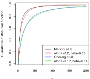
We have estimated α and β parameters, by comparing cumulative dis-tribution functions for read counts and Gamma (Figure 4.3). We found out that the best values for α andβ parameters were (0.2, 0.03) and (0.17, 0.01) for Marioni et al. and Cheunget al. data sets respectively.
4.3
Tools used for implementation
Affymetrix microarray data were processed using Affy package [81] from R/Bioconductor [82] and custom CDF files [31]. Microarray expression val-ues were summarized using RMA algorithm [30].
Sequencing data was converted from .sra format to .fastq format using SRA Toolkit version 2.1.9 [83]. Next, sequencing data was processed using three different methods: MMSEQ [9], RPKM [8] and PREBS.
To get MMSEQ gene expression measures, MMSEQ software (version 0.9.18) was used. Bowtie software (version 0.12.7) [46] was used to map the reads to the transcriptome, as recommended by MMSEQ manual. MMSEQ options were set to default and Bowtie options were set as recommended by MMSEQ (-a --best --strata -S -m 100 -X 400). Homo Sapiens tran-scriptome version GRCh37.65 from Ensembl database was used. SAMtools (version 0.1.18) [84] was used for alignment format conversion.
For the RPKM method, reads were mapped by TopHat software (ver-sion 1.4.1) [47]. Option --transcriptome-onlywas used for TopHat to get
Figure 4.3: Comparison of read count and Gamma cumulative distribution function
read alignments only to known transcriptome annotations. Ensembl GTF annotation file (version GRCh37.65) was used along with the genome file of the same version. Next, Ensembl genomic annotations were downloaded using GenomicFeatures package and read overlaps with gene regions were calculated using GenomicRanges package [85]. Then, RPKM values were calculated and base 2 logarithm values were taken.
PREBS values were calculated using the same tools as for RPKM values, but the read overlaps were calculated not for genes, but for probe regions taken from custom CDF file annotations. RMA algorithm was applied us-ing Affy package [81] slightly modified to accept custom probe expression measures.
All necessary data processing tasks were done using R, Perl and Python scripts. Script running was coordinated by Bash scripts. Additionally, some Unix shell utilities, such as grep, awk and sed, were used.
Results
In this chapter, we will introduce the results of the PREBS method and com-pare it against two other methods: MMSEQ and RPKM. In order to evaluate the methods, we will compare each of the method results against microar-ray results and calculate correlations. The methods will be tested in three different categories: absolute expression (Section 5.2), differential expression (Section 5.3) and cross-platform differential expression (Section 5.4). In ad-dition, we will have a look at some more technical results: we will examine our method performance using manufacturer’s CDF files instead of custom CDF files (Section 5.5) and we will calculate the differential expression for microarray replicates (Section 5.6).
5.1
Data sets
In our study we used two data sets: Marioni et al.[2] and Cheunget al [56]. These data sets were selected, because they were easily accessible, used popular sequencing and microarray platforms (Illumina and Affymetrix re-spectively). An additional advantage was that most of the samples in both datasets had microarray technical replicates which makes the data more re-liable.
The Marioni et al. [2] data set consisted of two samples: human kidney and liver. The sequencing was done using Illumina Genome Analyzer se-quencer for two runs where each of the runs was using 7 lanes. Some of the lanes contained 3 pM concentration while the others contained 1.5 pM concentration samples from human kidney or liver. We used only data from the lanes that contained 3 pM concentration. Altogether, there were 5 such lanes for the kidney sample and 5 such lanes for the liver sample. Each of these lanes gave 12.9-14.7 million 32 nucleotides long reads. The microarray
experiment was done using Affymetrix U133 Plus 2 platform. 3 microarray technical replicates were used for kidney and 3 for liver sample. Microarray and sequencing experiments were done on exactly the same samples using as similar sample preparation protocols as possible. The microarray data set is available in the GEO database [7] under accession number GSE11045 and sequencing data is available in NCBI short read archive under accession number SRA000299.
The Cheung et al. [56] data set consisted of 41 samples of B-cells taken from CEPH HapMap individuals. Illumina Genome Analyzer sequencer was used giving around 40 million 50 nucleotides long reads for each of the sam-ple. Microarray experiments were done using Affymetrix Human HG-Focus Target Array. 25 out of 41 samples had two microarray technical replicates while the rest of the samples did not have any microarray technical replicates. Sequencing and microarray samples were taken from the same individuals, hence, they were biological replicates. The data is available in the GEO database [7] under accession numbers GSE16921 and GSE16778 for sequenc-ing and microarray data, respectively.
We tried to find more coupled microarray–RNA-seq data sets, but it proved to be a difficult task. Most of the ones we found had some problems, for example, the microarray and RNA-seq samples were prepared in very different ways, old type of sequencing platforms were used or the data was not easily accessible. Therefore, in this thesis, we will only use the two aforementioned data sets.
5.2
Absolute expression comparison
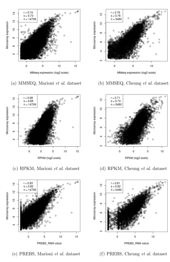
We have processed the RNA-seq data using 3 different methods: MMSEQ, RPKM and PREBS. Then, we processed microarray data for the same sam-ples using a single method—RMA. In order to find out which one of the 3 methods agrees best with microarray gene expression measurements, we have calculated Pearson and Spearman correlations and made scatter plots of microarray–RNA-seq data. We used 2 data sets: Marioni et al. [2] and Cheunget al.[56]. The scatter plots for all of the samples in each of the data sets looked similar, therefore, here we provide the scatter plots only for first sample in each data set: kidney sample in the Marioni et al. and GM06985 sample in the Cheunget al.data set (see Figure 5.1). On the other hand, the performance tables include the average correlations among all of the samples (see Tables 5.1, 5.2, 5.3 and 5.4).
For evaluation we used only those genes that were present on all of the RNA-seq processing methods and microarrays. Moreover, we filtered points
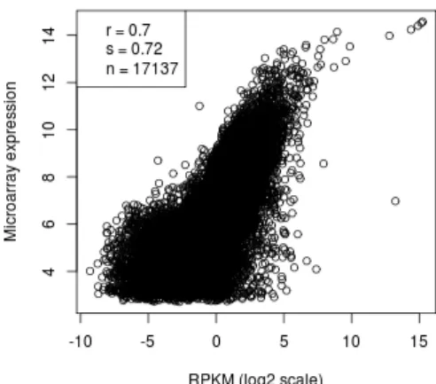
that had FPKM < 0.3 according to the MMSEQ method. The reason we did this is because MMSEQ measurements for low expressed genes are not very reliable and they decrease the correlation with microarrays quite a lot (see Figure 5.2). We also tried to filter low expression genes in RPKM and PREBS methods, but the correlation stayed virtually unaffected (data not shown), so we decided to include unfiltered results for these methods. In order to make the comparison fair, the three methods were evaluated on the exactly same set of genes.
From the scatter plots and the tables it is evident that PREBS agrees best with microarray data both in terms of Pearson and Spearman correlations. For the kidney sample in the Marioniet al. data set the Pearson correlations were 0.74, 0.68 and 0.83 for MMSEQ, RPKM and PREBS respectively (see Figures 5.1a, 5.1c and 5.1e). Similarly, for a GM06985 sample in the Cheung
et al. data set the Pearson correlations were 0.76, 0.71 and 0.81. Thus, PREBS performs best on both samples. The improvements in the correlation are just as evident when we look at Tables 5.1 and 5.2 where the correlations are averaged over all samples in the data sets (2 samples for the Marioni
et al. data set and 41 samples for the Cheung et al. data set). Pearson correlations for PREBS are 0.84 and 0.8, while for MMSEQ they are 0.7 and 0.76, for the Marioni et al.and the Cheunget al. data sets respectively. RPKM correlations are the lowest among all of the methods for both data sets.
Tables 5.3 and 5.4 show the correlation improvements of PREBS com-pared to other methods. The calculation formula for improvements was
(PREBS−OTHER)
(1−OTHER) · 100%, where PREBS is the correlation of PREBS vs mi-croarray and OTHER is the correlation of the other method vs mimi-croarray. The normalizing factor (1−OTHER) was chosen, because it corresponds to a total amount of how much correlation can be improved up until the perfect correlation.
Both for the Marioni et al. and the Cheung et al. data sets, PREBS reached reasonable amounts of improvement over the other two RNA-seq processing methods, but the improvement was bigger for the Marioni et al.
data set. The reason for that might have been, because RNA-seq and mi-croarray experiments for the Marioni et al. data set were conducted on ex-actly the same samples using very similar protocols, while for the Cheung et al. data set the RNA-seq and microarray samples were biological replicates which might have caused more differences in the expression levels. There-fore, the Marioni et al. data set is better suited for RNA-seq vs microarray comparisons and it is easier to reach some improvement in correlation using a novel method.
that have high microarray values (in the upper left corner). This effect is more evident for the Marioni et al. data set than the Cheung et al. data set. It is hard to tell what is the cause and it would require some further investigation. Interestingly, RPKM seems to be the only method for which this effect is not evident.
Moreover, in the plots for the Marioni et al. data set (Figures 5.1a, 5.1c and 5.1e) we see that expression values based on sequencing can go up even af-ter microarray values reach the saturation level. This suggests that RNA-seq has a larger dynamic range than microarrays. However, we cannot see such behaviour in the scatter plots for the Cheung et al. data set (Figures 5.1b, 5.1d and 5.1f).
(a) MMSEQ, Marioniet al.dataset (b) MMSEQ, Cheunget al.dataset
(c) RPKM, Marioniet al.dataset (d) RPKM, Cheunget al.dataset
(e) PREBS, Marioniet al.dataset (f) PREBS, Cheunget al. dataset
Figure 5.1: RNA-seq expressions plotted against microarray expressions. Kidney sample was used for the Marioni et al. dataset and GM06985 sam-ple was used for the Cheung et al. dataset. Points with FPKM < 0.3 were filtered. The legend contains Pearson correlation (r), Spearman correlation (s) and the number of genes (n).
(a) MMSEQ, Marioniet al.dataset (b) RPKM, Marioniet al. dataset
(c) PREBS, Marioniet al.dataset
MMSEQ RPKM PREBS Pearson 0.70 0.66 0.84
Spearman 0.68 0.64 0.83
Table 5.1: Absolute expression correlations for Marioni et al. dataset.
MMSEQ RPKM PREBS Pearson 0.76 0.71 0.80
Spearman 0.76 0.72 0.81
Table 5.2: Absolute expression correlations for Cheung et al. dataset.
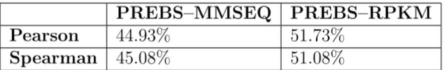
PREBS–MMSEQ PREBS–RPKM Pearson 44.93% 51.73%
Spearman 45.08% 51.08%
Table 5.3: Absolute expression correlation improvements comparing PREBS against MMSEQ and RPKM on Marioni et al. dataset.
PREBS–MMSEQ PREBS–RPKM Pearson 16.49% 29.48%
Spearman 18.35% 30.01%
Table 5.4: Absolute expression correlation improvements comparing PREBS against MMSEQ and RPKM on Cheung et al. dataset.
5.3
Differential expression comparison
In this section, we will compare differential expression measures between RNA-seq and microarray platforms. More precisely, we will compare differ-ences in log2 fold changes between the two platforms. We will not compare p-values or False Discovery Rate values, because these values in each platform are calculated in different ways and therefore they are not as comparable as log2 fold change values.
For the Marioniet al. data set log2 fold changes were calculated between liver and kidney samples. For the Cheung et al. data set we calculated log2 fold changes for several pairs of samples, but they were all quite similar, so we will include the results only for the pair of first two samples in the data set (GM06985 and GM06993).
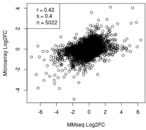
MMSEQ and RPKM vs microarray scatter plots (Figures 5.3a and 5.3c) look rather similar to the original scatter plot from the Marioni et al. publi-cation (Figure 3.1 on page 18). The Spearman correlations (0.74 and 0.75) are also similar to the one reported by the authors (0.75). MMSEQ and RPKM methods perform similarly both with respect to Pearson and Spear-man correlations. Unfortunately, the PREBS method (Figure 5.3e) did not significantly improve the differential expression correlations with microarray. Compared to RPKM, there is a small improvement for Pearson correlation (from 0.74 to 0.75), but there is no improvement for Spearman correlation.
Scatter plots for the Cheu
![Table 1.1: Number of microarray and RNA-seq experiments in ArrayEx- ArrayEx-press [6] database in the last three years](https://thumb-us.123doks.com/thumbv2/123dok_us/636541.2576690/8.892.165.449.195.266/table-number-microarray-experiments-arrayex-arrayex-press-database.webp)