Pattern Clustering using Soft-Computing Approaches

Pattern Clustering using

Soft-Computing Approaches

Mohit Agarwal

Department of Computer Science and Engineering

National Institute of Technology Rourkela

Pattern Clustering using Soft-Computing Approaches

Thesis submitted in partial fulfillment of the requirements for the degree of

Bachelor of Technology

in

Computer Science and Engineering

by

Mohit Agarwal

under the guidance of

Prof. S. K. Rath

NIT Rourkela

Department of Computer Science and Engineering

National Institute of Technology Rourkela

Department of Computer Science and Engineering

National Institute of Technology Rourkela

Rourkela-769 008, Orissa, India.

May 14, 2012

Certificate

This is to certify that the work in the thesis entitled Pattern Clustering Using Soft Computing Approaches by Mohit Agrawall is a record of an original research work carried out under my supervision and guidance in partial fulfillment of the requirements for the award of the degree of Bachelor of Technology in Computer Science and Engineering. Neither this thesis nor any part of it has been submitted for any degree or academic award elsewhere.

S. K. Rath

Acknowledgment

I express my sincere gratitude to Prof. S. K. Rath for his motivation during the course of the project which served as a spur to keep the work on schedule. I also convey my heart-felt sincerity to Ms. Swati Vipsita for her constant support and timely sugges-tions, without which this project could not have seen the light of the day.

I convey my regards to all other faculty members of Department of Computer Science and Engineering, NIT Rourkela for their valuable guidance and advices at appropri-ate times. Finally, I would like to thank my friends for their help and assistance all through this project.

Abstract

Clustering is the process of partitioning or grouping a given set of patterns into disjoint clusters. This is done such that patterns in the same cluster are alike and patterns belonging to two different clusters are different. . Clustering Process can be divided into two parts

• Cluster formation

• Cluster validation

The most trivial K-means algorithm is first implemented on the data set obtained from UCI machine repository. The comparison is extended to Fuzzy C-means algo-rithm where each data is a member of every cluster but with a certain degree known as membership value. Finally, to obtain the optimal value of K Genetic K-means algorithm in implemented in which GA finds the value of K as generation evolves.The efficieny of the three algorithms can be judged on the two measuring index such as : the silhouette index and Davies-Bouldin Index .

keywords: pattern clustering,soft computing,k-means,fuzzy c-means,genetic k-means,Silhouette index,Davies-Bouldin index

Contents

Certificate ii

Acknowledgement iii

Abstract iv

List of Figures vii

List of Tables viii

1 Introduction 1

1.1 Clustering . . . 1

1.2 Cluster Formation . . . 1

1.3 Cluster Validation . . . 2

2 Basic Concepts of Clustering 3 2.1 Cluster Validation . . . 3 2.1.1 Silhouette . . . 4 2.1.2 Davies-Bouldin Index . . . 5 2.2 Cluster Formation . . . 5 3 Clustering Algorithms 6 3.1 K-Means Algorithm . . . 6

3.2 Fuzzy C-Means Algorithm . . . 7

3.3 Genetic K-Means Algorithm . . . 8

4 Experimental Details 10 4.1 Iris Data Set . . . 10

4.2 Wisconsin Breast Cancer Data Set . . . 10

4.3 K-Means . . . 10

4.4 Fuzzy C-Means . . . 11

4.5 Genetic K-Means Algorithm . . . 11

5 Results and Discussions 12 5.1 K-Means Algorithm . . . 12

5.3 Genetic K-Means Algorithm . . . 17

6 Conclusion 19

List of Figures

5.1 Cluster formation using K-means on Iris dataset . . . 12

5.2 Cluster formation using K-means on Cancer dataset . . . 13

5.3 Silhouette Index of Iris dataset using K-means . . . 13

5.4 Silhouette Index of Cancer dataset using K-means . . . 14

5.5 clustering of iris data set using fuzzy c-means. . . 16

5.6 Silhouette Index of iris dataset using fuzzy c-means . . . 16

5.7 fuzzy c-means clustering of Cancer dataset . . . 17

List of Tables

5.1 Number of samples in cluster and its corresponding DBi

value for iris data set . . . 14 5.2 Number of samples in cluster and its corresponding DBi

value for cancer data set . . . 15 5.3 Silhouette index value for different number of clusters . . . 15 5.4 Davies-Bouldin index for different number of clusters . . . . 15 5.5 Silhouette index value for data sets . . . 18 5.6 Number of clusters obtained at different iterations. . . 18

Chapter 1

Introduction

Data Mining is the process of finding the pattern or relationship in the large data sets. This pattern or relationship can be coined as Knowledge, so the term Knowledge Discovery from Data, or KDD are used interchange-ably. This process involves use of automated data analysis technique to uncover the relationship between the data items. This data analysis tech-nique involves many different algorithms. The overall goal of the data mining process is to extract knowledge from an existing data set and trans-form it into a human-understandable structure for further use. The KDD process consists of various steps, they are data cleaning, data integration, data selection, data transformation, data mining, pattern evaluation and knowledge representation. The first four steps are different forms of data preprocessing, where data is prepared for data mining. The data mining step is an essential step where data analysis technique is applied to ex-tract patterns or knowledge. The exex-tracted patterns or knowledge is then evaluated in process evaluation step and this evaluated knowledge is the represented before the user in knowledge representation step. Basic data mining tasks are classification, regression, time-series-analysis, prediction, clustering, summarization, association rules and sequence discovery.

1.1

Clustering

Clustering is the unsupervised data mining technique partitioning or group-ing a given set of patterns into disjoint clusters without advance knowledge of the group or clusters. This is done such that patterns belonging to same clusters are alike and patterns belonging to two different clusters are dif-ferent. Clustering process can be divided into two parts, cluster formation and cluster validation.

1.2

Cluster Formation

Cluster formation is the process of placing the data elements in the related groups. This is done by the use of different algorithms. The algorithms

1.3 Cluster Validation Introduction

used are means algorithm, Fuzzy C-Means algorithm and Genetic K-Means algorithm.

1.3

Cluster Validation

Cluster validation is the process of measuring the quality of clusters formed. The cluster validation techniques used are Silhouette Index index and Davies-Bouldin Index.

Chapter 2

Basic Concepts of Clustering

Clustering is the process of partitioning the data elements into groups such that elements of the same group are alike or similar to each other and dis-similar to element of other group. Although classification is also process of partitioning data elements in groups such that element of same group are similar and dissimilar to other, but in this process, grouping is done on the basis of label of each element, which turns out to be costly. And this process of grouping is called supervised learning whereas clustering is un-supervised learning, where prior information of which element belongs to which group is not present. Clustering has various applications in various field like market research, pattern recognition, data analysis, bioinformat-ics, machine learning and image processing. The various cluster models are Connectivity model, Centroid model, Distribution model, Density model, subspace model and Graph-based model. Out of these data sets, Centroid model has been used for clustering. Clustering can be further classified as hard clustering and soft clustering. In hard clustering, each element sam-ple to exactly one cluster and in soft clustering, each element belong to each cluster to a certain degree. The hard clustering algorithm used in this project is K-Means and Genetic K-Means algorithm and soft computing algorithm used is Fuzzy C-Means algorithm.

2.1

Cluster Validation

After clusters are formed, cluster evaluation is the next and most impor-tant step. Based on its result the goodness of our cluster is decided, how well clusters are formed and data elements are grouped. The two criteria for cluster evaluation and selection of an optimal clustering scheme are compactness and selection. In compactness it is checked that members of each cluster should be as close to each other as possible. A common mea-sure of compactness is distance air dispersion, which should be minimized. In separation, the clusters themselves should be widely separated from each other. The common approaches for measuring the distance between the clusters are single linkage, complete linkage and comparison linkage.

2.1 Cluster Validation Basic Concepts of Clustering

In single linkage, separation is done on the basis of distance between the closest members of the cluster whereas in complete linkage, separation is done on the basis of distance between the most distant members and in comparison linkage separation is done on the basis of distance between the centers of the clusters. The various validation techniques are Silhou-ette Index index, Dunns index, Davies-Bouldin index and C-index. Out of these Silhouette Index index and Davies-Bouldin index have been used.

2.1.1

Silhouette

Silhouette Index refers to a method of interpretation and validation of cluster of data. The technique provides a succinct graphical representation of how well each object lies within its cluster. Intuitively, good clusters have the property that cluster members are close to each other and far from members of other clusters. For calculation of Silhouette Index the distance of cluster member with its other cluster member is found. The average distance between them is called dissimilarity. Cluster members with low dissimilarity are comfortably within the cluster to which they have been assigned. The average dissimilarity for a cluster is a measure of how compact it is. If the data set is divided into K clusters X=x1,x2,...,xj

, after applying some algorithm then for each datum i, a(i) is calculated, where, a(i) is the average dissimilarity of i with other data within the same cluster. The average dissimilarity of i is calculated with the data elements of other cluster and repeat this for every cluster of which i is not a member and lowest of this average dissimilarity is assigned as b(i).

By the value of a(i), it is interpreted how well that element is matched to the cluster it is assigned. Lower the value higher the matching. And from b(i), the cluster with minimum average dissimilarity is the neighboring cluster of i.s(i) is known as the Silhouette width. From its value it is determined how well the element is attached or matched to the cluster. The silhouette width,s(i), for the ith sample in the Xj cluster is defined as:

s(i) = b(i)−a(i)

max{a(i), b(i)}

Form the above definition it is clear the

−1≤s(i)≥1

When the value of s(i) is close to 1 then it is inferred that ith sample is well clustered. When it is close to 0 then it inferred that ith element can

be clustered to the neighboring cluster and when it is close to -1 then it inferred that element is misclassified i.e., it should have assigned to some other cluster. The silhouette index for a cluster is defined as average of sum of all the silhouette index of the members of that cluster,

Sj = 1 m m X i=1 s(i) 4

2.2 Cluster Formation Basic Concepts of Clustering

Where m is the number of elements in that cluster Sj.

The silhouette value for the whole system known as Global Silhouette GS is calculated as GSu =f rac1c c X j=1 Sj

Where c is number of cluster.

2.1.2

Davies-Bouldin Index

Davies-bouldin index aims at identifying the set of clusters which are com-pact and well separated. It is calculated as

DB =f rac1n n X i=1 max{Sn(Qi) +Sn(Qj) S(Qi, Qj) }

Where, Sn(Qi) is the average dispersion of the cluster which is calculated as Sn(Qj) = 1 Nj X x∈Cj ||x−mj||2

Where Nj is the is number of element in cluster j,and mj is the centroid

or cluster center of that cluster.

Small values of Davies-bouldin index conveys that cluster is compact and far away from other cluster.

2.2

Cluster Formation

Cluster formation is formation of clusters by applying some clustering algorithm on data sets. Clustering algorithm assigns data elements to some cluster thus dividing whole data set in groups. The algorithms used are K-Means, Fuzzy C-Means and Genetic Algorithm.

Chapter 3

Clustering Algorithms

3.1

K-Means Algorithm

The K-means algorithm is a typical partition-based clustering method which is simple and unsupervised. it is the basic partition algorithm which aims to partition n observations into k clusters in which each observation belongs to the cluster with the nearest mean. K in k-means is the number of cluster which is user input to the algorithm. It is iterative in nature.The K-means algorithm is simple and fast. The time complexity of K-means is (l*k*n), where l is the number of iterations and k is the number of clus-ters. Our empirical study has shown that the K-means algorithm typically converges in a small number of iterations.

The algorithm includes following steps:

Step 1: Choose K number of clusters which is predefined by user. Step 2: randomly choose k different clusters from the data set, which acts as the initial clusters for clustering.

Step 3: for each data elements compute the cluster which is closet to it and the assign that data element to that cluster.

Step 4: compute the new cluster center by taking the mean of all the elements in that cluster.

Step 5: repeat step 2-4 until there is no new assignments.

Computation of closet cluster is done by finding the euclidean distance between the data element and cluster center and assigned to that cluster with whom the euclidean distance is minimum.

Since k-means is simple and fast unsupervised clustering algorithm so it has some advantages and disadvantages.the advantages of using k-means algorithm are

1. Relatively efficient: where N is no. objects, K is no. clusters, and T is no. iterations. Normally, K, T ¡¡ N.

2. Procedure always terminates successfully i.e., given any numeric data set, k-means always gives a result such that all samples are divided into given number of clusters.

3.2 Fuzzy C-Means Algorithm Clustering Algorithms

The weakness of using k-means algorithm are

1. Does not necessarily find the most optimal configuration

2. Significantly sensitive to the initial randomly selected cluster centers 3. Applicable only when mean is defined (i.e. can be computed)

4. Need to specify K, the number of clusters, in advance which is a difficult task.

K-means is hard clustering type i.e., either a sample belong to this cluster or not. But there are some data elements which are present at the boundary of the cluster can belong to either of the cluster. So for this soft-computing approach is used for pattern clustering. In soft computing approach data are assigned a membership value which gives the amount of dependencies of that data element on different clusters and hence based on these membership value clustering is performed such that a data element can belong to two or more classes. So Fuzzy C-Means algorithm is used.

3.2

Fuzzy C-Means Algorithm

Fuzzy C-means (FCM) is a method of clustering which allows one piece of data to belong to more than one cluster. In other words, each data is a member of every cluster but with a certain degree of membership value. So each sample or element has some membership value so a sample is attached partially to other clusters also. So no cluster will be empty or no class will be with no data points. The output of such algorithm will be clustering but not partition. It is based on the minimization of the objective function Jm = N X i=1 C X j=1 uijm||xi−cj||2,1≤m <∞

Where m is any real number grater than 2,generally it is taken to be 2.uij

is the degree of membership of xi in j cluster,xi is the ith elements of the

cluster, cj is the centroid of the cluster j, C is the total number of cluster,

N is the total number of samples in the data set and ——*—— is norm for finding distance or similarity between two data and this is generally done by finding euclidean distance. Fuzzy partition is done by iterative optimization of the objective function and this iterative optimization is done by iterative findinguij and cj and then finding new objective function.

uij = 1 PC k=1( ||xi−cj|| ||xi−ck||) 2 m−1 , cj = PN i=1uijm·xi PN i=1uijm

And this iterative optimization is stopped when (uk+1-uk)¡e where e is a

value between 0 to 1. Algorithm steps:

3.3 Genetic K-Means Algorithm Clustering Algorithms

1. Initiate U=[uij] matrix, U(0)

2. At k-step calculate the centers vectors C(k)_=[c

j] with U(k) cj = PN i=1uijm·xi PN i=1uijm 3. Update U(k), U(k+1) uij = 1 PC k=1( ||xi−cj|| ||xi−ck||) 2 m−1

4. If || U(k+1) _{- U}(k) _{|| < then stop, otherwise return to step 2}

The advantages of using fuzzy c-means are:

1. No class or cluster will be empty. Every cluster will have some or partial membership of elements.

2. More efficient then k-means.

3. It has better convergence properties. Weakness of fuzzy c-means

1. For large data sets it consumes high CPU time.

2. Number of cluster is given in advance, before the execution of algo-rithm.

3. Sometimes it results into clusters but not partition. 4. Result depends on the initial cluster chosen.

3.3

Genetic K-Means Algorithm

The genetic algorithm is a probabilistic search algorithm that iteratively transforms a set (called a population) of mathematical objects (typically fixed-length binary character strings), each with an associated fitness value, into a new population of offspring objects using the Darwinian principle of natural selection and using operations that are patterned after naturally occurring genetic operations, such as crossover (sexual recombination) and mutation.

In GAs, the parameters of the search space are encoded in the form of strings (called chromosomes). A collection of such strings is called a popu-lation. Initially, a random population is created, which represents different points in the search space. An objective and fitness function is associated with each string that represents the degree of goodness of the string. Based on the principle of survival of the fittest, a few of the strings are selected

3.3 Genetic K-Means Algorithm Clustering Algorithms

and each is assigned a number of copies that go into the mating pool. Bi-ologically inspired operators like cross-over and mutation are applied on these strings to yield a new generation of strings. The process of selection, crossover and mutation continues for a fixed number of generations or till a termination condition is satisfied.

Basic Genetic Algorithm Steps: 1. Representation:

The value of K is chosen such that it lies between [kmin,kmax],where kmin is

the minimum number of cluster to be formed. Generally it is taken as 2 unless specified. Andkmax is the maximum number of cluster to be formed,

which is taken to be length of the string. —bf 2. Population initialization:

K random cluster centers are chosen and places in random order in the string and the remaining places are filled with NULL. Thus one chromo-some is formed. And this step is repeaated for each chromochromo-some of the population Chosen.

3. Fitness Computation:

Fitness computation is the most crucial part of genetic algorithm. In this algorithm inverse of davies-bouldin index is used as fitness value.

4. Selection

After fitness is computed for each chromosome , they are sorted in de-scending order and the top kmax/2 is selected for mutation and crossover.

5. Crossover

The selected chromosomes are then single point cross overred with the probability of Pc.

6. Mutation

After the crossover mutation is done on the population set to generate new set of population. Mutation is done with the probability of Pm. (Pm*kmax*no.of chromosome) values are randomly selected from the pop-ulation and then checked, if the value is null then select a value randomly from the data set and replace that null value with it else if value is not null then is made null.

Chapter 4

Experimental Details

The data set used for various clustering algorithms as an input are: 1. Iris Data Set

2. Wisconsin Breast Cancer Data Set

which are obtained from UCI Machine Repository.

4.1

Iris Data Set

This is perhaps the best known database to be found in the pattern recog-nition literature. The data set contains 3 classes of 50 instances each, where each class refers to a type of iris plant. Every sample of iris data set have four attributes, which are sepal length, sepal width, petal length and petal width. One class is linearly separable from the other 2; the latter are NOT linearly separable from each other.

4.2

Wisconsin Breast Cancer Data Set

The data set contains 2 classes with distribution of 458 in one class and remaining 241 in other one. Every sample of Wisconsin breast cancer data set have 10 attributes, which are Sample code number, Clump Thickness, uniformity of Cell Size, Uniformity of Cell Shape, Marginal Adhesion, Sin-gle Epithelial Cell Size, Bare Nuclei, Bland Chromatin, Notmal Nucleoli, Mitoses.

4.3

K-Means

Since benchmark data set are used, so number of clusters are known in advance. The results obtained from experiment is then compared with the existing one. Number of clusters of Iris Data set are 3 and of Wisconsin breast Cancer Data set is 2.

4.4 Fuzzy C-Means Experimental Details

4.4

Fuzzy C-Means

The membership function uij is chosen as number of cluster × number of

samples. And its data are assigned randomly in the range of 0 to 1. The end result or the partition depends on this initial membership matrix.

4.5

Genetic K-Means Algorithm

The control parameters used in Genetic k-Means are 1. Population size(N)=10

2. Probability of crossover(Pc)=0.5

3. Probability of mutation(Pm)=0.1

4. Size of chromosome=10

5. Maximum number of generations=200 6. Crossover:Single point

Chapter 5

Results and Discussions

5.1

K-Means Algorithm

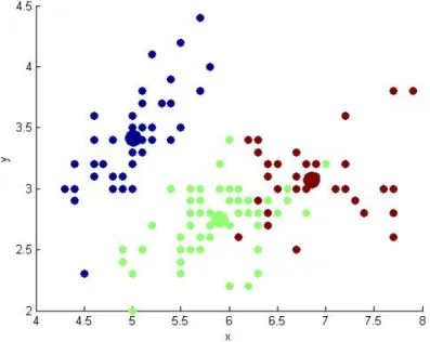
On applying k-means on the data sets the clusters formed are seen below. The dot represent the samples and final centroid of the cluster is shown by the bigger dot in size.The dots of same colour belong to one cluster with bigger dot as its centroid. The X-axis and y-axis are the first two attributes which are plotted in Cartesian space.

Figure 5.1: Cluster formation using K-means on Iris dataset

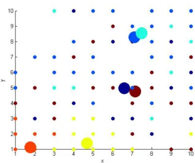
5.1 K-Means Algorithm Results and Discussions

Figure 5.2: Cluster formation using K-means on Cancer dataset

The silhouette index for these data sets are

5.1 K-Means Algorithm Results and Discussions

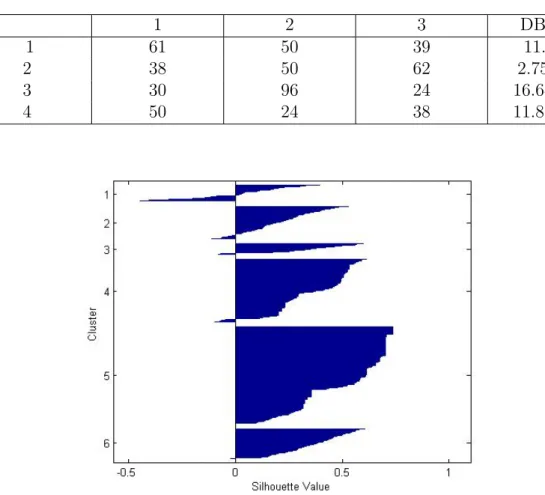
Table 5.1: Number of samples in cluster and its corresponding DBi value for iris data set 1 2 3 DB 1 61 50 39 11.43 2 38 50 62 2.75 3 30 96 24 16.64 4 50 24 38 11.87

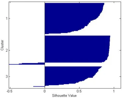
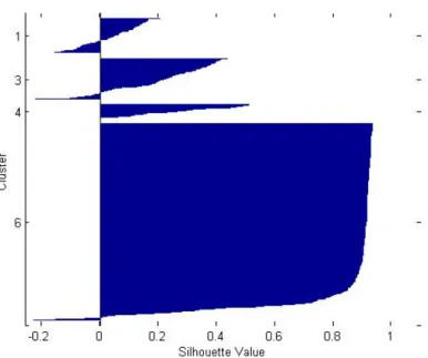
Figure 5.4: Silhouette Index of Cancer dataset using K-means

The above figures represent the Silhouette Index index. In figure (iris) it is observed from the graph that value of Silhouette Index is lying in the range of 0.8 to 1, which means that the clusters are well formed, compact and distant from each other. in the second figure(cancer)for some cluster 1 the positive value is lying around 0.5, means it is semi compact and negative value is also around 0.5 means some elements are misclassified i.e., there are some elements in cluster 1 which shouldnt be present in cluster 1. For cluster 5 it is observed that Silhouette Index value is lying in the positive side, means it is perfectly clustered.

The Davies-bouldin index for

The above figure displayed the number of samples in each cluster for iris data set after different iterations and its corresponding Davies-Bouldin index. As discussed earlier, less the Davies-Bouldin index value, better is the cluster formed. And from the above table it is noticed that Davies-Bouldin index is minimum for 2nd iterations, so it can be said that cluster formation with data element distribution as (38,50,62) is a better cluster-ing. These number in different cluster varies at different iterations because of choosing initial cluster centroid as random. So initial centers plays an

5.1 K-Means Algorithm Results and Discussions

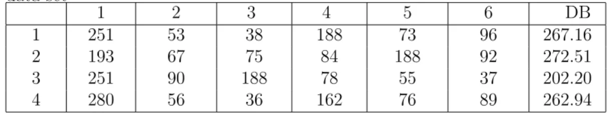
Table 5.2: Number of samples in cluster and its corresponding DBi value for cancer data set 1 2 3 4 5 6 DB 1 251 53 38 188 73 96 267.16 2 193 67 75 84 188 92 272.51 3 251 90 188 78 55 37 202.20 4 280 56 36 162 76 89 262.94

Table 5.3: Silhouette index value for different number of clusters

no.of cluster iris cancer

2 .8502 .7542

3 .7355 .7542

4 .6786 .3083

5 .6722 .6162

6 .5772 .3775

important role in clustering.

From this table also it is concluded that cluster 3 is the best cluster formed with (251,90,188,78,55,37) as distribution of data elements in clus-ters.

Cluster validation also provides insight into the problem of predicting the correct numbers of clusters. So by analyzing the value of the various in-dexes it can predicted the number of clusters for that data set such that, the inter-cluster distance and intra-cluster distance is maximum and min-imum respectively. As the value of Silhouette Index should be more for better cluster formation and Davies-Bouldin index should be less.

From the above figure it is conclude that if Silhouette Index index is considered then the value of K i.e., number of cluster, will be that value whose corresponding Silhouette Index is maximum and that comes out to be 2 in case of iris and 2 in case of cancer. But if Davies-Bouldin index is considered then that cluster will be selected whose corresponding Davies-Bouldin index value is minimum and that comes out to be 2 in case of iris data set and 3 in case of Wisconsin breast cancer data set. And this obtained k value is used in k-means algorithm.

Table 5.4: Davies-Bouldin index for different number of clusters

no.of cluster iris cancer

2 7.91 33.46

3 19.10 26.42

4 15.56 28.27

5 48.59 260.93

5.2 Fuzzy C-Means Algorithm Results and Discussions

5.2

Fuzzy C-Means Algorithm

Figure 5.5: clustering of iris data set using fuzzy c-means

Figure 5.6: Silhouette Index of iris dataset using fuzzy c-means

5.3 Genetic K-Means Algorithm Results and Discussions

Figure 5.7: fuzzy c-means clustering of Cancer dataset

Figure 5.8: Silhouette Index of Cancer dataset using fuzzy c-means

5.3

Genetic K-Means Algorithm

Since benchmark data set has been used from UCI machine repository so the number clusters that data set should have formed. So our obtained result is compared from the existing value. K value for iris data set is 3 and value obtained from our Genetic K-Means algorithm is in range of 4-6, which is close. Similarly for Wisconsin breast cancer data set, the K

5.3 Genetic K-Means Algorithm Results and Discussions

Table 5.5: Silhouette index value for data sets

no.of cluster iris cancer

2 .8502 .7542 2 .7358 .7525 3 .4891 .6618 4 .4445 .4769 5 .4891 .4385 6 .5970 .5562

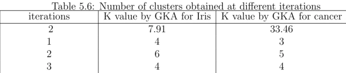
Table 5.6: Number of clusters obtained at different iterations iterations K value by GKA for Iris K value by GKA for cancer

2 7.91 33.46

1 4 3

2 6 5

3 4 4

value is 2 and our obtained value is in range of 3-5 which is also close. So it is concluded that genetic K-Means algorithm gives the K value which is close to original number of cluster that data set should have formed.

Chapter 6

Conclusion

Though K-means algorithm is easy to implement but to determine the value of K at prior is a difficult task. Many number of iterations were performed to determine the optimal value of K which was a very time consuming process. From the above implementations, it can be concluded that the K value obtained from Genetic K-means is very near to the exact number of clusters. The genetic K means algorithm globally partitions the data set into a specified number of clusters. Fuzzy C-Means algorithm partitions each sample in clusters but in this algorithm no class or cluster lies empty. So, it can be concluded that in Genetic K-means no initial guess of probable number of clusters is required, but the final output is very close to the exact number of clusters.

Bibliography

[1] Fu-Lai Chung & Shitong Wang Lin Zhu. Generalized fuzzy c-means clustering

algorithm with improved fuzzy partitions. IEEE Transactions on Systems, Man,

and Cybernetics, Part B: Cybernetics, 39:578–591, 2009.

[2] Jitendra V.; Bezdek James C. Cannon, Robert L.; Dave. Efficient implementation of the fuzzy c-means clustering algorithms. IEEE Transactions on Pattern Analysis and Machine Intelligence, PAMI-8:248–255, 1986.

[3] Ming-Chuan Hung; Don-Lin Yang;. An efficient fuzzy c-means clustering algorithm. Proceedings IEEE International Conference on Data Mining, pages 225–232, 2001.

[4] A.B. Gath, I.; Geva. Unsupervised optimal fuzzy clustering. IEEE Transactions on

Pattern Analysis and Machine Intelligence, 11:773–780, 1989.

[5] Wang Min; Yin Siqing. Improved k-means clustering based on genetic algorithm. In-ternational Conference on Computer Application and System Modeling, ICCASM, 2010.

[6] Ujjwal Maulik; Sanghamitra Bandyopadhyay. Genetic algorithm-based clustering

technique. Pattern Recognition, 33:1455–1465.

[7] K. Krishna ; M. Narasimha Murty. Genetic k-means algorithm. IEEE

TRANSAC-TIONS ON SYSTEMS, MAN, AND CYBERNETICSPART B: CYBERNETICS, 29, 1999.

[8] Bashar Al-Shboul; Sung-Hyon Myaeng. Initializing k-means using genetic

algo-rithms. World Academy of Science, Engineering and Technology, 2009.

[9] Madjid Khalilian; Norwati Mustapha; MD Nasir Suliman ; MD Ali Mamat. A novel

k-means based clustering algorithm for high dimensional data set. International

Multiconference of Engineers and Computer scientists, Vol I,TMECS 2010:104– 109, 2010.