Fairness scheme for energy efficient H.264/AVC-based video sensor network

R E S E A R C H

Open Access

Fairness scheme for energy efficient

H.264/AVC-based video sensor network

Bambang AB Sarif

, Mahsa T Pourazad

, Panos Nasiopoulos

, Victor CM Leung

and Amr Mohamed

* Correspondence:

[email protected]

1_{Electrical and Computer} Engineering Department, University of British Columbia, 2332 Main Mall, Vancouver, BC V6T 1Z4, Canada Full list of author information is available at the end of the article

Abstract

The availability of advanced wireless sensor nodes enable us to use video processing techniques in a wireless sensor network (WSN) platform. Such paradigm can be used to implement video sensor networks (VSNs) that can serve as an alternative to existing video surveillance applications. However, video processing requires tremendous resources in terms of computation and transmission of the encoded video. As the most widely used video codec, H.264/AVC comes with a number of advanced encoding tools that can be tailored to suit a wide range of applications. Therefore, in order to get an optimal encoding performance for the VSN, it is essential to find the right encoding configuration and setting parameters for each VSN node based on the content being captured. In fact, the environment at which the VSN is deployed affects not only the content captured by the VSN node but also the node’s performance in terms of power consumption and its life-time. The objective of this study is to maximize the lifetime of the VSN by exploiting the trade-off between encoding and communication on sensor nodes. In order to reduce VSNs’ power consumption and obtain a more balanced energy consumption among VSN nodes, we use a branch and bound optimization techniques on a finite set of encoder configuration settings called configuration IDs (CIDs) and a fairness-based scheme. In our approach, the bitrate allocation in terms of fairness ratio per each node is obtained from the training sequences and is used to select appropriate encoder configuration settings for the test sequences. We use real life content of three different possible scenes of VSNs’implementation with different levels of complexity in our study. Performance evaluations show that the proposed optimization technique manages to balance VSN’s power consumption per each node while the nodes’maximum power consumption is minimized. We show that by using that approach, the VSN’s power consumption is reduced by around 7.58% in average.

Keywords:Component; Video sensor network; H.264/AVC; Power consumption; Computation and communication trade-off; Fairness

Introduction

The advances in VLSI, sensors and wireless communication technologies have pro-vided us with miniature devices that have low computational power and communica-tion capabilities. These devices can be organized to form a network called wireless sensor network (WSN). A WSN is typically used to measure physical attributes of the monitored environment and send the information to a central device that usually has unlimited resources. The information gathered at the central device, usually called the sink node, can be used by human operator or any additional machine/software to

several existing surveillance technologies because it can be implemented in an ad-hoc manner, customized to user requirements, and implemented on locations that are lack-ing infrastructure. However, unlike the conventional WSNs, VSNs require a large amount of resources for encoding and transmitting the video data. Therefore, maximiz-ing the power efficiency of codmaximiz-ing and transmission operations in VSNs is very important.

Video nodes in VSNs share the same wireless medium in order to send their encoded video to the sink node. Since the bandwidth allocated for the network is limited, there is an issue of fairness of bandwidth allocated per each VSN node. Allocating the same bitrate to each video node guarantees the fairness in terms of bitrate and the quality of the encoded video, given that each node is using the same video encoding parameter settings and configurations. However, in many VSN deployment scenarios, nodes fur-ther from the sink usually need to relay their data through intermediate nodes. There-fore, the total energy consumption of nodes that are closer to the sink will be greater than the nodes further. More balanced energy consumption among VSN nodes is achieved by allocating different fairness ratio per each node in the VSN. It has to be noted that this has to be done without sacrificing the quality of the transmitted video of any node. To this end different fairness ratios are assigned to VSN nodes such that the tradeoff between encoding complexity and compression performance is exploited. Since encoding complexity and compression performance (in terms of bit rate) deter-mine the required power for coding and transmission respectively, assigning different fairness ratio per each node will affect the distribution of power consumption in a VSN. To the best of our knowledge this idea has not been studied in details in the existing literature on VSN.

energy consumption in a VSN. Furthermore, in [12] some encoder parameters that can affect the performance of the encoder in terms of bitrate and computational complexity were highlighted. In order to take advantage of the trade-off between encoding and transmission energy consumptionin, a table called configuration ID (CID) was pro-posed, that includes several encoder configuration settings to compress a video with almost similar quality in terms of peak signal to noise ratio (PSNR), at different bitrate and compression complexity level. Unlike the CommonConfig approach used in [10] [11], where all VSN nodes have the same encoding configuration, the proposed scheme in [12], assigns different CIDs to different nodes in order to exploit the trade-off between communication and computation. The analysis of the energy consumption fairness of the VSN showed that by assigning different configuration setting parameters to each node, the node’s maximum energy consumption of VNSs can be reduced [13]. One of the common drawbacks of the existing studies is using the same video resource for all VSN nodes. While this seting may show some aspects of the video encoding process and trade-off in a VSN, it does not reflect the real life setting of a VSN deploy-ment, where different VSN nodes capture the scene from different point of view and thus the complexity of captured content is not consistent over different nodes. Note that the performance of a video encoder in terms of computational complexity and bitrate depends on both the encoding configuration and temporal and spatial complex-ity of content. That brings the problem of exploiting the trade-off between computation and communication in a VSN into a different level of difficulty.

In this paper, we propose an algorithm to reduce the maximum power consumption VSN nodes by extending our previous work in [12] and [13]. We use a branch and bound optimization techniques on a finite set of CID options and a fairness-based scheme in order to reduce VSNs’ power consumption and obtain a more balanced energy consumption among VSN nodes. Furthermore, in order to simulate a realistic VSN implementation, we use a variety of real life captured content in our analysis. We also study the effect of spatial and temporal complexity of the videos on the VSN’s encoding performance. In order to perform the analysis, the captured videos are classified into different content complexity classes. Then some of these videos are used for training and the rest for testing the performance of our algorithm. Also, to evaluate the performance of the proposed algorithm in a more realistic scenario, the VSN used in this study has a more complex network topology than the one used in [12,13].

The rest of the paper is organized as follows: Section Video capturing and encoding settings describes the video capturing and encoding settings used in this paper, Section Video content classification presents the video content classification methodology, Section VSN Power consumption modelling and formulation describes the energy con-sumption model for the VSN used in the paper, experiments and results are provided in Section Experiments and results, and conclusions are and future works are discussed in Section Conclusions.

Video capturing and encoding settings

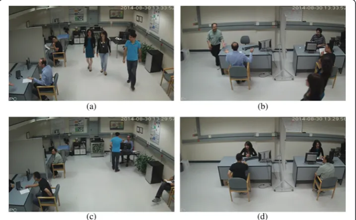
such that each of them has different field of view as shown in Figure 1. Some of the cameras’ field of view overlaps one another. The scene arrangement is such that the motion and activities are not centered in the middle of the field and the content cap-tured by each camera is different. With the assumption that most important activities occur around the entrance door in a surveillance system, the middle camera (see cam-era 5 in Figure 2) is directed towards the door. To capture representative VSN data with different temporal and spatial complexity levels, we modify the layout of the lab to

Figure 1Camera placements.In order to mimic a realistic scenario, nine cameras are installed in one of our lab such that each of them has different field of view.

represent three different scenes, namely “office”, “classroom”, and “party”. Figure 2 il-lustrates the layout of different scene settings. To have a representative database with different activity levels, each scene is captured several times based on four different settings as follows:

1. The level of activity of all the people in the room is high, and the total number of people is between six to eight.

2. Three or more people moving around the room, while the total number of people in the room is around six.

3. Couple of people walking around the room, while the total number of people in the room is around five.

4. Three or four people walking in the room.

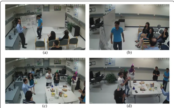
Using the nine cameras installed, we have captured four different activity settings for the three scenes (“office”, “classroom” and “party”), producing 108 different videos to be used for our analysis. Each video is 10s length and downsampled to 15 frame per seconds (fps) 416×240 pixels to mimic the requirement of a decent video sensor net-work. Figure 3 shows snapshots of the“office”scene from camera2 and camera4 when activity level of the scene falls into the first and third settings. As it is observed the video content from the two cameras and the two activity scenarios are not the same. Figure 4 shows snapshots from the “classroom” and “party” scenes when the activity level of the scene falls into the second setting. For ease of referencing, the following video identification is used: <camera-id__scene-setting__activity-level>. Hence, cam-era2_party_act1 means the video captured by camera2 in the “party” scene when the activity level of the scene falls into the first setting.

Figure 3Some snapshots from the“office”scene.The first row show the snapshots of the“office” scene in the first activity settings from:(a)camera2 and(b)camera6. The two cameras produced different contents when the activity level of the scene falls into the third setting as shown in(c)camera2 and

For encoding the videos captured at each node, we use the most widely used video coding standard H.264/AVC [6]. The video coding standard comes with a number of different encoding tools that can be configured to suit a wide range video applications. The performance of the H.264/AVC encoder in terms of computation requirement (complexity) and bitrate depends on the setting parameters used to encode the video. One of the encoding parameters is group of picture (GOP) size. GOP size determines the number of frame coded picture within a successive video stream. In inter-frame prediction process, each block within a current inter-frame is predicted by the most similar block from previously coded reference frames. This is in contrast with the intra-frame prediction technique, in which blocks of pixels are predicted from its neighboring pixels within the same frame. The inter-frame prediction technique pro-duces lower bitrate than intra-frame prediction; while the encoding complexity of inter-frame coding is much higher than the later. As it is observed by increasing the GOP size, the number of inter-frame coded pictures increases, therefore the bitrate of the coded video is reduced at the cost of higher encoding complexity. Note that the complexity and bitrate of inter-frame prediction can be controlled by adjusting the search range (SR) of motion estimation process. The SR determines the size of search-ing area in the reference frame to find the best match to be used for inter prediction. Increasing the SR may result in better compression performance at the cost of in-creased complexity. However this observation is quite content dependant and there are cases where increasing the value of SR does not provide significant benefit in terms of compression performance [12]. Quantization parameter (QP) is another encoding par-ameter that regulates how much spatial detail is saved. In fact, the quality of the encoded video in terms of peak signal to noise ratio (PSNR) depends largely on the QP value. When QP value is very small, the residue signal is preserved more and the qual-ity of compressed video is high, at the cost of higher complexqual-ity and bitrate.

Due to the limitation in the energy and processing resources of VSNs, less complex encoder configurations are deployed. To this end, we use the baseline profile of H.264/ AVC that is suitable for low complexity applications. Therefore, only I and P frames are used (no B-frame). The other encoding settings used in this paper include the use of context-adaptive variable-length coding (CAVLC) entropy coding, one reference frame, SR equal to eight, while the rate distortion optimization (RDO), rate control, and the deblocking filter are disabled. The H.264/AVC reference encoder software (JM 18.2) is used in our study. The instruction level profiler iprof [14] that provides us with the number of basic instruction counts (IC) to perform an encoding task is used as the en-coding complexity measure. The benefit of using IC as the measure of complexity is threefold. Firstly, IC is more accurate than the commonly used encoding time. The other benefit of using IC is the fact that IC is agnostic to the device architecture. In addition, IC can be used to estimate the encoding power consumption of the video node.

From our earlier work, we learned that the IC increases as the GOP sizes increases [12]. For a specific QP, however, increasing the GOP size will also reduce the bitrate as the number of intra predicted frames are reduced. Therefore, the trade-off between en-coding and transmission power consumption can be controlled by managing the GOP size. This information were translated into a tabular format as shown in Table 1. It has to be noted that the table only shows the value of GOP size used for the corresponding configuration ID (CID). The remaining encoder setting parameters are the same, i.e., as mentioned in the previous paragraphs.

Figure 5(a) shows the complexity and bitrate plot of the CIDs defined in Table 1 for different QP values forcamera2_party_act2video. As it is observed, when CID value is small, the compression performance of the encoder is sacrificed such that the bitrate is high. However, this is compensated by having a low encoding complexity. On the other hand, using bigger CID means increasing the encoder complexity to gain a better com-pression performance. Figure 5(a) also shows that reducing the value of QP will in-crease both the encoder complexity and bitrate. Therefore, the bitrate of the encoded video and the complexity of the encoding process depend on the CID and QP used. It has to be noted that although the GOP sizes gap for CID = 6 (GOP = 32) and CID = 7 (GOP = 64) is very high, i.e., the GOP size gap is 32, the different in complexity (bitrate) between these two CIDs is very small. Moreover, the values used in Table 1 shows a re-lation between the GOP size and the CID, i.e.,CID = log2(2*GOP). This shows that the CID values represent an encoder parameter, i.e., the GOP size, whose values affect the complexity and bitrate of the encoder. We also want highlight that the bitrate

Table 1 Configuration ID (CID)

CID GOP

1 1

2 2

3 4

4 8

5 16

6 32

(complexity) is monotonously decrease (increase) with the increase of CID value. In terms of the encoded video quality, Figure 5(b) shows that for the same QP, the quality of the encoded video is almost the same in terms of PSNR, i.e., the different is less than 0.5 dB, regardless of the CID value used to encode the video.

Video content classification

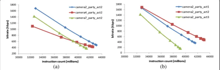
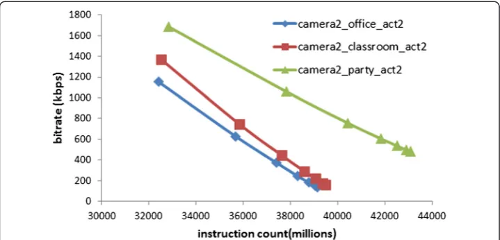
Since the cameras in a VSN can have different field of views, the content captured by each camera in a VSN will be different. For example, Figure 6(a) shows the complexity and bitrate of videos captured by three different cameras in the “party” scene at the same activity level while Figure 6(b) shows the complexity and bitrate of videos cap-tured by camera2 in the “party” scene at different activity levels. On the other hand, Figure 7 shows the complexity and bitrate of videos captured by camera2 in different scenes. It can be seen from these figures that the bitrate and encoding complexity of the videos captured by each camera depends on the content complexity of the scene. The video that contain more objects and with higher motion will have a higher bitrate than the video that has less objects and motion. Consequently, the total bitrate gener-ated by the captured scenes that have high spatial and temporal detail will be bigger

Figure 5Complexity, bitrate, and video quality trade-off.Part(a)of this figure shows the trade-off between complexity (in terms of instruction counts) and bitrate ofcamera2_party_act2video encoded with different CID and QP values. It can be seen that the smaller CID value entails high bitrate but low encoding complexity. On the other hand, encoding the video with a smaller QP value (to get better video quality) increases computation complexity and bitrate. Part(b)of the figure shows that for the same value of QP, the video quality is almost the same, regardless of the CID used to encode the video.

than the ones obtained from the scenes with lower spatial and temporal detail. Ideally, we need to find the nodes’optimal bitrate allocation for each possible scene. However, this approach is not practical. In this regard, we assume that if we can obtain the opti-mal bitrate ratio allocation for the worst scenario, i.e., when the nodes’ bitrate is high, we can use that information as an initial guide for us to allocate the configuration set-tings for the other scenarios. Thus, in this paper, the scenes with higher content will be used for the training set while the remaining scenes are use as the test set. In order to find the scenes that have higher activity content, we need to formulate a methodology to classify each camera and scene into different content complexity level. For that pur-pose, we use the ITU-T recommendation that includes the use of spatial information unit (SI) and temporal information unit (TI) that is defined as follow [15]:

SI ¼ maxtime stdspace½Sobel Fð Þn

ð1Þ

T I¼ maxtime stdspace½Fn−Fn−1

ð2Þ

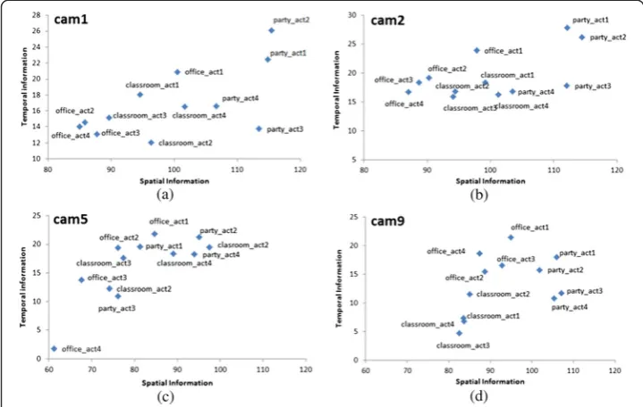
SI and TI measure the spatial and temporal activity level of videos. In this regard, Figure 8 shows the SI and TI values of camera1, camera2, camera5, and camera9. It can be seen from this figure that for the same scene, each camera has different spatial and temporal activity level. Consequently, Table 2 shows the SI values of all videos while Table 3 shows the TI values, respectively.

In order to classify the scenes into different content complexity level, the following procedure is used:

1. Classify each video from a scene into different SI and TI classes using the following threshold:

t1¼mean CCð Þ−0:5std CCð Þ t2¼mean CCð Þ þ0:5std CCð Þ CC ¼fSI;T Ig

Using (3), we found that the value of t1and t2 for SI are 87.85 and 98.95, respect-ively. On the other hand, the value oft1andt2for TI are 14.32 and 19.04, respectively. For example, if a specific video’s SI is less thant1, the video is classified aslow-SI_video. If the video’s SI is higher thant2, it is classified ashigh-SI_video. If the video’s SI is be-tweent1andt2, the video is classified asmedium-SI_video.

2. Based on the SI(TI) classes of the videos, we classify the scene into different SI(TI) classes using the following rules:

a. The SI(TI) class of a scene is equal to the majority of SI(TI) classes of all videos from that scene

b. If no majority is found, the scene is classified as medium SI(TI) scene Figure 8Spatial and temporal information of all scenes captured.The figure shows the spatial and temporal information captured from(a)camera1,(b)camera2,(c)camera5, and(d)camera9.

Table 2 Spatial Information unit (SI) of all videos

Scene cam1 cam2 cam3 cam4 cam5 cam6 cam7 cam8 cam9 office_act1 100.52 97.83 88.92 76.17 84.60 89.95 85.73 95.06 94.98

office_act2 85.83 90.26 85.90 71.24 76.14 84.45 85.20 90.06 88.62

office_act3 87.78 88.68 89.78 74.30 67.62 91.16 89.93 90.80 92.75

office_act4 84.97 87.01 87.96 71.40 61.17 89.97 83.85 87.36 87.43

classroom_act1 94.62 99.18 96.73 89.56 97.46 96.04 92.03 88.12 83.59

classroom_act2 96.30 94.46 96.30 91.46 74.07 88.83 92.74 85.52 84.99

classroom_act3 89.67 94.11 90.04 85.71 77.42 87.03 88.94 85.85 82.55

classroom_act4 101.69 101.21 94.74 92.68 89.08 94.57 91.86 89.19 83.64

party_act1 114.85 112.10 116.85 99.60 81.27 104.73 104.60 110.79 105.97

party_act2 115.40 114.49 107.53 90.61 95.06 101.31 104.56 111.56 101.90

party_act3 113.43 112.04 113.87 99.02 76.15 96.36 107.40 111.86 107.08

Figure 9 shows an example on how to obtain the office_act1 and classroom_act1 scenes’ classes. Using the above rule, the office_act1is classified as medium-SI_high-TI_scene. On the other hand, scene classroom_act1is classified as medium-SI_medium-TI_scene. Figure 10 shows the classes of all the scenes.

Scenes with high SI will generally produce videos with higher bitrate than the scenes that have lower SI. This is especially true for CID equal to one that corresponds to using GOP size equal to one, i.e., the video is intra-frames coded. Therefore, the config-uration settings that is suitable for a specific SI class may not be suitable to be used for the other SI class. Based on this assumption, the scenes are arranged into three differ-ent sets, namely scenes that have high SI, scenes that have medium SI and scenes that have low SI. In each of these sets, the scene with the highest TI will be selected as the training scene. For example, in Figure 10, the scenes having medium SI are the offi-ce_act1, office_act3, classroom_act1, classroom_act2, and classroom_act4. Out of these five scenes, the scene that has the highest TI class, i.e., office_act1, is selected as the training scene for the medium SI scenes. If there is more than one candidate for the training scene, the scene that has the biggest average TI will be selected as the training scene. Henceforth, the training set for the high SI scenes is theparty_act2, the training set for the medium SI scenes is the office_act1, and the training scene for the low SI Table 3 Temporal Information unit (SI) of all videos

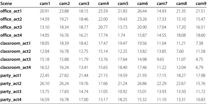
Scene cam1 cam2 cam3 cam4 cam5 cam6 cam7 cam8 cam9 office_act1 20.91 23.88 18.15 25.59 21.83 26.44 14.93 21.35 21.51

office_act2 14.59 19.21 18.46 22.00 19.43 23.26 17.33 15.10 15.47

office_act3 13.10 18.34 18.77 20.77 13.73 20.90 17.04 17.20 16.51

office_act4 14.05 16.76 16.21 17.74 1.74 15.87 14.55 18.08 18.60

classroom_act1 18.05 18.39 18.42 17.47 19.47 19.56 11.04 11.21 7.38

classroom_act2 12.04 16.78 12.75 15.14 12.25 13.82 13.85 7.60 11.58

classroom_act3 15.18 15.88 11.79 13.76 17.64 14.98 9.65 11.07 4.75

classroom_act4 16.52 16.24 13.41 15.65 18.40 17.46 11.22 12.04 6.79

party_act1 22.45 27.82 21.44 27.15 19.59 21.93 17.15 18.27 17.98

party_act2 26.10 26.24 19.76 17.66 21.24 26.86 22.29 22.67 15.76

party_act3 13.75 17.83 14.74 17.05 10.92 15.01 13.93 13.50 11.72

party_act4 16.59 16.78 17.00 13.17 18.25 15.32 11.10 13.31 10.83

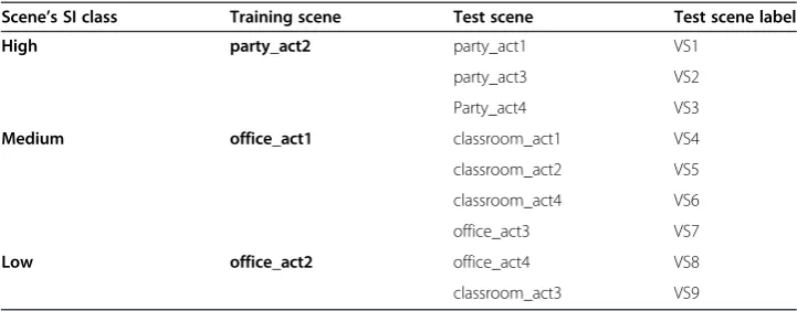
scenes is the office_act2. The training scenes are shown in bold in Figure 10. Corres-pondingly, Table 4 shows the training scenes and their corresponding test scenes.

VSN Power consumption modelling and formulation

The encoding power consumption of a VSN node depends on the CID value assigned to that node. However, since some nodes need to relay their data through intermediate nodes, the node’s communication power consumption depends on both the CID value assigned to that node and the way the encoded data is relayed in the network. This problem can be formulated as an optimization procedure. For this purpose, the follow-ing video sensor node model is used in this paper. All the nodes, includfollow-ing the sink, are assumed to be statically deployed in the deployment area. It is assumed that a standard medium access control (MAC) protocol is applied to resolve the link interfer-ence problem. The network is modeled as an undirected graph G(N,L) whereNis the set of nodes andLis the set of links. The nodes are identified such that the first node is the closest node to the sink while the Nthnode is farthest one. The sink has unlim-ited source of energy. However, the total information flow to the sink is constrained by the bandwidth of the network.

Nodeican communicate with nodejif a link between those nodes (Lij∈L) exists. Sen-sor nodeican capture and encode video, and then generate video traffic with a source rate Ri. Furthermore, each node can also relay the traffic from upstream nodes. The flow conservation law at each node is then:

X

rij− X

rki¼Ri ð4Þ

Figure 10Scene’s classes.The scenes shown in bold are the training scenes for their respective SI class.

Table 4 Training and test scenes

Scene’s SI class Training scene Test scene Test scene label High party_act2 party_act1 VS1

party_act3 VS2

Party_act4 VS3

Medium office_act1 classroom_act1 VS4

classroom_act2 VS5

classroom_act4 VS6

office_act3 VS7

Low office_act2 office_act4 VS8

Here, rijdenotes the outgoing rate atLij whilerkidenotes incoming rates at Lki, and

Lij,Lki∈L.

The sum of transmission rate of all the nodes is constrained to be equal to the band-width available (B):

XN

i¼1Ri≤B ð5Þ

The bitrate allocated to a node itself is obtained using the relationRi=R{CIDi,QPi}, whereRis the bitrate of the video for the pair ofCIDandQPused by the node.

A generally used energy consumption model for a wireless communication transmit-ter and receiver as presented in [16] is used in this paper. The total transmission power consumption of node i is the sum of all power consumed to transmit data to other nodes within its transmission range. The transmission power consumption is calculated as follow:

Pti¼ X

aþβ⋅dijn

⋅rij ð6Þ

where, Pti is the transmission power consumption of node i, α and β are constant coefficients, η is the path loss exponent, and dij is the distance between node i and node j. The total reception power consumption of nodeiis the sum of all power con-sumed to receive data from other nodes, as formulated below, where λ is a constant coefficient:

Pri¼ X

λ⋅rki: ð7Þ

The energy depleted to execute that task can be calculated as the multiplication of the total number of cycles to execute that task and the average energy depleted per cycle. Therefore, the average power consumption required to encode a sequence is estimated as [12]:

Pei¼

ki⋅CPI⋅Ec⋅Fr Nf

ð8Þ

where, κiis the total number of instructions to encode the video for node i,CPIis the average number of cycles per instruction of the CPU, Ec is the energy depleted per cycle, Nfis the number of frames andFrdenotes the frame rate of the video sequence. The value of κi is obtained using the following relationκi=IC{CIDi, QPi}, where ICis the instruction count provided by iprof for the pair ofCIDand QP values used. Since we want each node to produce video with almost similar quality, all nodes have to use the sameQP, thus,QPi=QP,∀i∈N.

The total energy dissipation at a sensor node consists of the encoding power consumption (Pe), the transmission power consumption (Pt) and the reception power consumption (Pr):

Pi¼PeiþPtiþPri ð9Þ

Pei¼Ki⋅CPI⋅Eec⋅Fr=Nf

Ki¼IC CID i;QP X

rij− X

rki¼Ri;∀k∈N;k≠i;∀j∈N;j≠i

Ri¼R CIDf i;QPg

Pti¼ X

aþβ⋅dn_i

⋅rij

Pri¼ X

λ⋅rki_;∀k∈N;k≠i X

Ri≤B

In order to find the configuration settings per each node that minimizes the energy consumption, we need to evaluate all possible CID combinations in the VSN. Letvi de-notes the different CIDs that can be used by node i, thenV= {v1,v2,…,vN} denotes the vector of possible CID that can be selected by the nodes in a VSN. The combination of all CIDs that needs to be evaluated is then given byC(V,N), whereCdenotes the com-binatorial operation. The number of possible combinations increases with the number of node. For example, when the number of nodes is equal to three, the number of pos-sible CID combinations that needs to be evaluated is equal to 343. However, when the number of nodes is increased to nine, the number of possible CID combination is equal to 79. We can reduce the search space for the optimization problem by focusing on the fact that all nodes share the same wireless bandwidth (2) such that the bitrate allocated per each node is equal to a portion of the total bandwidth. Therefore, the problem of assigning the CIDs to all nodes can be viewed as the problem of assigning fairness ratio to each node in the VSN.

Common approach

A common approach for setting encoding parameters of VSN nodes is to use the same configuration settings over all nodes. We call this approach CommonConfig algorithm. This approach has been used by [10] and [17] to analyze the VSN power consumption of Intra only configuration and Inter Main Profile with GOP size of 6 and frame-type sequence of I-P-B-P-B-P-I. The authors in [11] also have used CommonConfig algorithm for Intra only configuration in their analysis. In order to implement the CommonConfig algorithm while still being fair with the implementation reported in the literature, we try to assign the same CID to all nodes such that the bandwidth con-straint is not violated.

each node will have the same bitrate and encoding complexity. However, if the video source for each video is different, assigning the same CID to each node will not guarantee the same bitrate is allocated to each node. The amount of bitrate allocated to each node will then depend on the content complexity of the video captured by the node. To guaran-tee some fairness measure for the VSN nodes, one can allocate the same bitrate per each node. In this regard, the end-to-end fairness constraint, i.e., the maximum percentage of the total bitrate that can be sent to the sink by each node, is formulated as follow [18]:

Ri≤ρi⋅

XN

j¼1R_j ð10Þ

With this constraint, each node ican only generate a flow to the sink that is lower than a fraction of ρi of the sum of the bitrate of all nodes. According to (5) the sum of all bitrate has to be less than the bandwidth of the network (B). When all nodes use the same fairness constraints that is equal to ρfair=ρi= 1/N, each node will be allocated equal transmission rate. In this condition, the network is called to use the MaximumFairness scheme, as shown below.

In the algorithm shown above, the procedure getCIDis a procedure to assign a node with a specific CID, where R{CIDi, QP}/B<ρi, andRis the bitrate allocated for nodei when using the corresponding CID. Note that, fratio= {ρ1,ρ2,..ρN}, N is the number of nodes, andρi= 1/N.

Proposed optimization-based minimum energy VSN

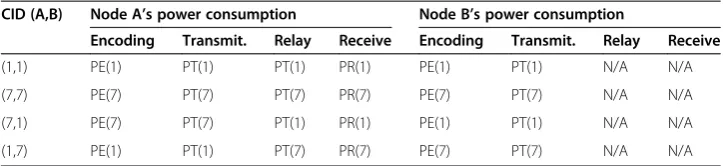
using a particular CID for a specific video. The table shows that if both nodes use the same CID, the power consumption of node A will be higher than that of node B. However, if the nodes are using different CIDs, we can exploit trade-off between encoding complex-ity and bitrate to minimize the node’s maximum power consumption. The example shown in the Table is for a simple VSN with two nodes. However, the number of possible CID combinations increases exponentially with the increase of the number of nodes.

Furthermore, it should be noted that the value of CID is bounded to be integral. On the other hand, the value of rijand rkithat determine the routing of data from and to node i in (6) and (7) are rational numbers. An optimization problem involving mixed linear and integer variables is NP-complete, where some of the solutions are intract-able. However, there are algorithms that can be used to provide a near optimal solution for this kind of optimization problem. These algorithms mostly work by solving the re-laxed linear programming and then adding some linear constraints that drive the solu-tion towards being integer without excluding any integer feasible points. Branch and bound [19] is considered one such algorithm. Using branch and bound algorithm, the optimization procedure can be terminated early and as long as a solution that satisfies the stopping criteria is found. Therefore, a feasible, not necessarily optimal solution can be obtained. In this paper, the branch and bound approach is implemented by using the following steps: 1) solve the bounded optimization problem 2) call a recursive pro-cedure to perform branch and bound until a solution is found or termination criteria are satisfied. The bounded optimization problem is shows as follow.

Optimization minimizePowerBounded(CIDu_bound,CIDl_bound) minimize Pnet

subject to:

Pi≤Pnet

Pi¼PeiþPtiþPri Pei¼κi⋅CPI⋅Eec⋅Fr=Nf κi¼IC CIDf i;QPg X

rij− X

rki¼Ri;∀k∈N;k≠i;∀j∈N;j≠i Ri¼R CIDf i;QPg

Pti¼ X

αþβ⋅dη_i

⋅rij Pri¼

X

λ⋅rki;∀k∈N;k≠i X

Ri≤B

CIDi≤CIDu boundi CIDi≥CIDl boundi

values are given as upper and lower bounds instead of a specific value. Note that, since the CID value represent the configuration label, whenever the optimization procedure needs to lookup the values of the complexity and bitrate, the CID value needs be rounded to the nearest integer. If the CID provided by the bounded optimization does not satisfy the inte-grality constraint, the RecursiveBranchBound procedure will be called to perform branch and bound approach to find the solution, as shown below.

If a solution that satisfies the integrality constraint cannot be found, the prob-lem will be divided into two sub-probprob-lems by defining new upper and lower bounds followed by call to the recursive functions. Note that, the integrality con-straint ε is the error between the CID and the rounded integral value of the CID. In order to illustrate the proposed approach, consider an example of a four node Table 5 Node’s power consumption for a simple scenario

CID (A,B) Node A’s power consumption Node B’s power consumption

Encoding Transmit. Relay Receive Encoding Transmit. Relay Receive

(1,1) PE(1) PT(1) PT(1) PR(1) PE(1) PT(1) N/A N/A

(7,7) PE(7) PT(7) PT(7) PR(7) PE(7) PT(7) N/A N/A

(7,1) PE(7) PT(7) PT(1) PR(1) PE(1) PT(1) N/A N/A

Fairness-based CID allocation for the test Set

The scenes’content complexity affects the overall VSN’s power consumption. Ideally, in order to find the best solution, the VSN nodes’optimal bitrate for each possible scene has to be calculated. However, this approach is not practical since the scene’s activity captured by a VSN changed with time while the algorithm to find the optimal solution requires some significant computation. Thus, following our assumption mentioned in Section Video content classification, we will attempt to find the optimal fairness ratio allocation only for the training sets. The optimal fairness ratio allocation obtained from the training sets will be used as an initial guess to allocate the CID for the test videos. However, since the content of the video of the training set and the test set are not exactly the same, we need to perform some adjustment procedure while assigning the nodes’CID in the test sets. Hence, the algorithmFairnessBasedCID allocation is shown below.

will return CID equal to six. However, in some cases, thegetCID procedure may not be able find a suitable CID with fairness ratio allocation ρj to be allocated to node j. In this regard, the node will need to be assigned the highest CID possible accord-ing to Table 1, i.e., it will use the configuration with the lowest bitrate. Then, a vari-able named overflow is updated with the difference between the allocated bitrate (obtained using a lookup table R{CIDj, QP}) with the supposed maximum bitrate for that node, i.e.,ρj*B. Note that, the variableoverflowis used to record the accumula-tive amount of bitrate that are borrowed from the other nodes. On the other hand, if an appropriate CID is available while the value of overflow variable is positive, an-other call to the procedure getCID with a lower fairness ratio is performed to get another CID. This is performed so that we can ‘pay back’ the outstanding bitrate ‘debt’. The overflow variable is then updated accordingly. In the chance that the overflow variable is still positive after the CID allocation for all nodes have been per-formed, a procedure checkBandwidthConstraint is then called to adjust the CID al-location per each node. Starting from the node furthest from the sink, the procedure checks whether assigning a higher CID to that node can reduce the variableoverflowto be less than or equal to zero. After that, the nodes’power consumption is calculated using the minimizePower procedure as discussed in Section VSN Power consumption modelling and formulation.

Figure 11Example of how the proposed optimization based approach proceeds.This figure shows an example of CID allocation for a four node VSN. Part(a)of the figure shows the initial step where the solution obtained is shown as the dark bold line. Since the solution violates the integrality constraint, the search space is divided into two new spaces, colored with green and yellow. Then, recursive calls with new boundaries are executed. Following the assumption shown in Table 6, the new solution is shown as the dark bold line in(b). Here two new search spaces are created. Note that, in this figure, the upper and lower bound for the yellow colored space is the same.

Table 6 Example of the progression of the proposed MILP-based optimization for a four node VSN

Bounds Solution found

Step 1 UB = {4,4,4,4} SOL = {3.5, 2.75, 2, 1.75}

LB = {1,1,1,1}

Recursive 1 UB = {4,4,4,4} NA

LB = {4,3,3,2}

Recursive 2 UB = {3,2,2,1} SOL = {2.75, 1.75, 1.75, 1}

LB = {1,1,1,1}

Recursive 2.1 UB = {3,2,2,1} SOL = {3, 2, 2, 1}

LB = {3,2,2,1}

Recursive 2.2 UB = {2,1,1,1} SOL = {2,1,1,1}

In this algorithm, the perturb procedure checks whether altering the CID allocation of a specific node can reduce the VSN’s power consumption. For example, if nodei is assigned to use CID equal to four, the perturb procedure will check whether assigning CID equal to three or five to nodeireduces the VSN’s power consumption further.

Experiments and results

This section elaborates on our experiment settings for evaluating the performance of our proposed approach. To ensure the efficiency of our proposed scheme, our experiment re-sults are compared with the CommonConfig and MaximumFairness approaches.

Experiments settings

Figure 12 is attached to the camera located at the same location shown in Figure 1. Therefore, node1 will be using the video captured by camera1; node2 will be using the video captured by camera4, and so forth. The H.264/AVC software, JM version 18.2 is used to generate the CID lookup table of encoding complexity and bitrate of all videos. The QP value used in this paper ranges from 28 until 36.

Two separate sets of experiments were performed. The first set of experiment is con-ducted on the training set. The objective is to compare the results obtained by the pro-posed optimization technique with the ones obtained using the CommonConfig and MaximumFairness approaches. From this experiment, we will obtain the fairness ratios of the training set that minimize the node’s maximum energy consumption. We will compare the energy consumption obtained using that approach with the one obtained using the CommonConfigandMaximumFairness approaches. To this end the parame-ters shown in Table 7 are used.

Performance evaluation of the proposed algorithms for the training scenes

In order to find the minimum power consumption with the highest possible video qual-ity, we need to find the minimum QP for each content complexity class. To do this, starting from the lowest QP, a procedure to check the possibility to allocate CIDs to all the nodes is performed using the MaximumFairness approach. Since each scene has different SI (TI) complexity class, the minimum QP value for each scene may also be different. For example, for scene party_act2, the minimum QP that can be used to allocate the CID using the maximum fairness approach is equal to 36. However, the

minimum QP for scene office_act2is 28. Once the minimum QP for a scene is ob-tained, we execute the optimization-based approach on the corresponding training scene. It should be noted that for the optimization-based approach, we repeat the experiment eight times to find the best solution. For the purpose of the analysis, we compare the performance of the algorithm against the CommonConfig and Maxi-mumFairness approaches mentioned in Section Common approach. Figure 13 shows the bitrate allocated using the compared techniques. Figure 13(a) shows the bitrate allocation for the training scenes obtained using the CommonConfig algo-rithm. The figure shows that the difference between the highest bitrate and the lowest bitrate allocated in each scene is as follow: 129.85 kbps for the high SI train-ing scene (party_act2), 115.87 kbps for the medium SI training scene (office_act1)

Figure 13Bitrate allocated per each node in all training scenes.Part(a)of the figure shows the bitrate allocated by theCommonConfigapproach. Part(b)of the figure shows the bitrate allocated by the MaximumFairnessapproach. The figure shows that the bitrate allocated per each node is roughly the same. On the other hand,(c)shows the bitrate allocated by the proposed optimization based.

B Network Bandwidth 2 Mbps

d Distance between node 5m

and 115.08 kbps for the low SI training scene (office_act2), respectively. The algorithm CommonConfigdoes not regulate the bitrate assigned per each node since the algorithm only concern about using the same configuration for each node. Thus, the bitrate assigned to each node does not follow any trend. However, the MaximumFairnessapproach allo-cates roughly the same bitrate per each VSN node for any training scene used as shown in Figure 13(b). Given that the content captured by each camera in each training scene is not the same, there are some variations in the bitrate assigned to each node. However, the dif-ference between the highest bitrate and the lowest bitrate allocated in each scene is not significant, i.e., 50.37 kbps for the high SI training scene (party_act2), 63.85 kbps for the medium SI training scene (office_act1) and 41.64 kbps for the low SI training scene ( offi-ce_act2), respectively. On the other hand, the proposed optimization-based approach takes into account the node’s total power consumption in allocating the bitrate for each node. As Figure 13(c) shows, the proposed technique allocates different bitrate to each node such that the nodes closer to the sink have generally higher bitrate than the nodes that are farther from the sink. The different between the maximum and minimum bitrate allocated in each scenes has become more significant, equaling to 327.73 kbps for the high SI scene, 471.56 kbps for the medium SI scene and 476.59 kbps for the low SI training scene, respectively. It can also be seen in this figure that node2 is allocated with smaller bitrate than the other nodes. The reason behind this behavior is the fact that node2 corre-sponds to camera4 (see Figure 1), which according to Table 2 and Table 3 has lower con-tent complexity level than the other cameras.

balanced, we can obtain lower VSN’s power consumption than the other algorithms. Fur-thermore, Table 9 shows the fairness ratio allocation of the training scenes.

Performance of the fairness based algorithms for the test scenes

Using the fairness ratio obtained from the training scenes, the fairness based algorithm explained in Section Fairness-based CID allocation for the Test Set will be used to allo-cate the VSN nodes’ CID for all test scenes. Our initial experiments show that the fairness-based with adjustment algorithm managed to obtain lower Pnet, Pavg and STD (Pi) than the propsoed fairness-based allocation algorithm. Therefore, from this point forward, we will only compare the proposed fairness-based with adjustment with the other techniques mention in Section Common approach. In this regard, Table 10 shows the Pnet, Pavgand STD(Pi) of the three algorithms for all test scenes. It can be seen from the table that the proposed fairness with adjustment algorithm proves to perform better than the other techniques. Correspondingly, Figure 15 compares the value of the Pnet, Pavg and STD(Pi) obtained by the three algorithms in all test cases. Furthermore, Table 11 shows the percentage of Pnet, Pavgand STD(Pi) improvement obtained by the proposed techniques against the common approach for all test cases used. It can be seen here that the amount of power consumption reduction obtained by the proposed fairness-based with adjustment technique is in the range of 5.06% to 10.48%, averaging into 8.18% improvement against the MaximumFairness algorithm. On the other hand,

Table 8 Pnet, Pavgand STD(Pi) of the training scenes

Training sequence

Pnet Pavg STD(Pi)

Common Config Maximum Fairness Proposed Common Config Maximum Fairness Proposed Common Config Maximum Fairness Proposed

party1_act2 10.73 10.95 9.73 9.40 9.39 9.31 0.54 0.64 0.18

office_act1 10.25 10.45 9.53 9.03 9.03 9.38 0.49 0.57 0.09

office_act2 9.97 10.06 9.35 8.80 8.83 9.19 0.47 0.48 0.09

ric

Computin

g

and

Informa

tion

Sciences

(2015) 5:7

Page

25

of

9.67%, averaging into 6.97% improvement. Thus, the average improvement of the proposed algorithm against the common approach is around 7.58%. This result is encouraging since it shows that by using the fairness ratio obtained from the videos with higher activity level; we are still able to reduce the maximum power consumption by around 7.58% than the CommonConfigandMaximumFairnessapproaches. Since VSN’s energy is usually limited, reducing the energy consumption by 7.58% means that we are increasing the lifetime of the sensor network by 7.58%. In addition to that, except for test scene VS1 and VS4 the proposed algorithm also manage to slightly reduces the average power consump-tion. On the other hand, the standard deviation of nodes’power consumption is also reduced by more than 40% on average.

Future work

In order to improve the result obtained in this paper, there are some considerations that can be included into our framework. The first and notable extension is to directly incorporate the effect of spatial and temporal information of the videos into the

Figure 15Comparison of the Pnet, Pavg, and STD(Pi) values obtained from all test scenes.This figure compares the Pnet, Pavg, and STD(Pi) values obtained by the(a)CommonConfig(b)MaximumFairness(c)

optimization framework. In this paper, the effect of spatial and temporal information is implemented indirectly through the process of classifying the videos into different scenes’classes. We are currently working on to develop a model for encoding complex-ity and bitrate that incorporate the spatial and temporal information. By using a model, we can remove the use of tabular information of configuration ID that is used in this paper. Another consideration that could be addressed is the power consumption minimization during or at the point of the transmission. For example, one can imple-ment an importance based scheduling approach such that only select nodes are allowed to send their data to the sink. Some other practical considerations that could be in-cluded from this study is to consider the effect of camera orientation into the VSN power consumption and whether the nodes are implemented for indoor or outdoor en-vironment. We are also considering the possibility to use the new encoding standard HEVC for our future work. However, it has to be noted that HEVC encoder’s complex-ity is higher than that that of H.264/AVC encoder. HEVC utilizes more advanced and complex features compared to H.264/AVC. In order to implement our approach to the HEVC-based VSNs, we need to first investigate the trade-off provided by different en-coding parameters of HEVC and generate a CID table customized for HEVC, and then tune our scheme accordingly.

Table 10 Performance of the different techniques in all test cases

Test scenes

CommonConfig MaximumFairness Proposed

Pnet Pavg STD(Pi) Pnet Pavg STD(Pi) Pnet Pavg STD(Pi)

VS1 10.61 9.32 0.55 10.87 9.41 0.63 9.73 9.35 0.26

VS2 10.47 9.18 0.56 10.56 9.19 0.62 10.03 9.14 0.41

VS3 10.63 9.22 0.59 10.71 9.24 0.64 9.60 9.16 0.24

VS4 10.11 8.78 0.58 10.48 8.99 0.67 9.40 8.89 0.36

VS5 10.08 8.73 0.58 10.08 8.77 0.59 9.28 8.66 0.34

VS6 10.14 8.79 0.58 10.29 8.87 0.62 9.38 8.76 0.34

VS7 9.73 8.84 0.37 9.91 8.83 0.45 9.29 8.78 0.23

VS8 9.55 8.51 0.43 9.64 8.52 0.47 9.04 8.43 0.29

VS9 10.06 8.76 0.57 10.07 8.80 0.58 9.24 8.69 0.33

Table 11 Percentage of improvement of the proposed algorithm against the other techniques

Test scenes Improvement against CommonConfig (%) Improvement against MaximumFairness (%) Pnet Pavg STD(Pi) Pnet Pavg STD(Pi)

VS1 8.33 −0.29 51.92 10.48 0.72 58.20

VS2 4.24 0.41 26.68 5.06 0.48 33.54

VS3 9.67 0.63 60.32 10.30 0.88 63.30

VS4 7.01 −1.29 38.01 10.23 1.04 46.57

VS5 7.88 0.83 40.86 7.97 1.29 41.32

VS6 7.50 0.41 41.89 8.83 1.29 45.48

VS7 4.60 0.63 36.85 6.28 0.53 47.90

VS8 5.40 0.96 33.65 6.21 1.05 38.81

maximum power consumption is then used on the training sets. We have shown that the proposed optimization procedure performs better than the CommonConfig and MaximumFairness approaches such that VSN’s power consumption per each node was balanced while the nodes’ maximum power consumption is minimized. We have also shown in this paper that the fairness ratio allocated per each node affects the distribu-tion of power consumpdistribu-tion in a VSN. In particular, by assuming that the fairness ratio of nodes closer to the sink are higher than the nodes that are farther from the sink, the VSN’s power consumption is reduced.

The fairness ratio obtained by the proposed optimization-based approach is then used in the proposed fairness-based encoder complexity and bitrate allocation algo-rithm for the test scenes. The results show that the amount of power consumption reduction obtained by the proposed techniques varies according to the test sequences used. In general, the improvement obtained by the fairness based with adjustment tech-nique is 8.18% on average against the MaximumFairnessalgorithm and 6.97% on aver-age against CommonConfigalgorithm. In addition to that, the proposed algorithm also shows better performance in terms of nodes’average power consumption and standard deviation of nodes’power consumption.

Abbreviations

WSN:Wireless sensor network; VSN: Video sensor network; CID: Configuration ID; PSNR: Peak signal to noise ratio; FPS: Frames per second; GOP: Group of pictures; SR: Search range (in motion estimation); QP: Quantization parameter; IC: Instruction counts; SI: Spatial information unit; TI: Temporal information unit; CPI: Cycle per instruction.

Competing interests

The authors declare that they have no competing interests.

Authors’contributions

This work is a joint effort between the University of British Columbia and Qatar University. All authors have contributed to this document and given the final approval. All authors read and approved the final manuscript.

Acknowledgment

This work was supported by the NPRP grant # NPRP 4-463-2-172 from the Qatar National Research Fund (a member of the Qatar Foundation). The statements made herein are solely the responsibility of the authors.

Author details

1_{Electrical and Computer Engineering Department, University of British Columbia, 2332 Main Mall, Vancouver, BC V6T} 1Z4, Canada.2TELUS Communications Inc, 555 Robson St, Vancouver, British Columbia V6B 3K9, Canada.3Computer Science and Engineering Department, Qatar University, Doha, Qatar.

Received: 20 November 2014 Accepted: 12 February 2015

References

1. Akyildiz F, Melodia T, Chowdhury KR (2007) A survey on wireless multimedia sensor networks,”Computer Networks. The International Journal of Computer and Telecommunications Networkin 51(4):921_–960 2. Ren X, Yang Z (2010)“Research on the key issue in video sensor network”, presented at the Computer Science

and Information Technology (ICCSIT), 2010 3rd IEEE International Conference on. Chengdu 7:423_–426 3. Seema A, Reisslein M (2011) Towards efficient wireless video sensor networks: a survey of existing node

4. Chen J, Safar Z, Sorensen JA (2007) Multimodal Wireless Networks: Communication and Surveillance on the Same Infrastructure. Information Forensics and Security, IEEE Transactions on 2(3):468–484

5. R¨aty TD (2010) Survey on Contemporary Remote Surveillance Systems for Public Safety,”Systems, Man, and Cybernetics, Part C. Applications and Reviews, IEEE Transactions on 40(5):493–515

6. Wiegand T, Sullivan GJ, Bjontegaard G, Luthra A (2003) Overview of the H.264/AVC video coding standard. IEEE Transactions on Circuits and Systems for Video Technology 13(7):560–576

7. Richardson E (2010) The H.264 Advanced Video Compression Standard, Second Editionth edn. John Wiley & Sons, Ltd 8. H. K. Zrida, A. C. Ammari, M. Abid, and A. Jemai, Complexity/Performance Analysis of a H.264/AVC Video Encoder,

in Recent Advances on Video Coding, InTech, Rijeka, Croatia, 2011.

9. Ostermann J, Bormans J, List P, Marpe D, Narroschke M, Pereira F et al (2004) Video coding with H.264/AVC: tools, performance, and complexity. IEEE Circuits and System Magazine 4(1):7–28

10. J. J. Ahmad, H. A. Khan, and S. A. Khayam,“Energy efficient video compression for wireless sensor networks,” Information Sciences and Systems, 2009. CISS 2009. 43rd Annual Conference on, Baltimore, MD, 2009, pp. 629– 634.

11. Imran N, Seet BC, Alvis C, Fong M (2012) A comparative analysis of video codecs for multihop wireless video sensor networks. Multimedia Systems 18(5):373–389

12. B. A. B. Sarif, M. T. Pourazad, P. Nasiopoulos, and V. C. M. Leung,“Encoding and communication energy consumption trade-off in H.264/AVC based video sensor network,”World of Wireless, Mobile and Multimedia Networks (WoWMoM), 2013 IEEE 14th International Symposium and Workshops on a , pp.1,6, Madrid, 4-7 June 2013. 13. B. A. B. Sarif, M. T. Pourazad, P. Nasiopoulos, and V. C. M. Leung,“Analysis of Energy Consumption Fairness in

Video Sensor Networks.”Poster presented at 2013 Qatar Foundation Annual Research Forum Proceedings, ICTSP 02. Qatar, Nov. 2013.

14. P. M. Kuhn,“A Complexity Analysis Tool: iprof (version 0.41),”ISO/IEC JTC1/SC29/WG11/M3551, Dublin, Ireland, July 1998.

15. ITU-T,“Subjective video quality assessment methods for multimedia applications,”P.910, April 2008. 16. T. S. Rappaport, Wireless communications: principles and practice, 2nd ed. Prentice Hall, 2001.

17. S. Ullah, J. J. Ahmad, J. Khalid, and S. A. Khayam, "Energy and distortion analysis of video compression schemes for Wireless Video Sensor Networks," Military Communication Conference, MILCOM 2011, Baltimore, MD, Nov. 2011, pp. 822–827.

18. B. Krishnamachari and F. Ordonez,“Analysis of Energy-Efficient, Fair Routing in Wireless Sensor Networks through Non-linear Optimization,”in IEEE Vehicular Technology Conference, 2003 IEEE 58th, vol.5, Orlando, Florida, Oct. 2003, pp. 2844–2848.

19. J. Clausen,“Branch and Bound Algorithms - Principles and Examples,”University of Copenhagen, Mar. 1999. 20. D. Chinnery and K. Keutzer, Closing the Power Gap between ASIC & Custom: Tools and Techniques for Low

Power Design, 1st edition. Springer, 2007.

Submit your manuscript to a

journal and benefi t from:

7Convenient online submission 7Rigorous peer review

7Immediate publication on acceptance 7Open access: articles freely available online 7High visibility within the fi eld

7Retaining the copyright to your article