Existence And Uniqueness Of The Adjoint Function For Degree-One Approximation: Dasguptas Approach

912

Existence And Uniqueness Of The Adjoint

Function For Degree-One Approximation:

Dasgupta’s Approach

Rishabh Tiwari, P. L. Powar

Abstract— Dasgupta, proposed a method to construct the wedge functions over an element of polygonal discretization of the domain using an analytic approach to determine the denominator of rational wedge function, whereas Wachpress had applied the geometric approach for the same task. We have extended the idea described by Dasgupta and established the conditions, mandatory for the existence and uniqueness of the denominator and consequently the wedge functions in case of the quadrilateral discretization of the domain. A more general form of the linear functions, representing sides of the quadrilateral has been considered, which eradicates restriction on the sides for not passing through the origin. This paper has been furnished with a Mathematica program which computes all the required parameters and finally approximation over the element under consideration.

Index Terms—. Finite Element, Quadrilateral Discretization, Rational Form, Adjoint, athematica

——————————  ——————————

1 I

Finite Element Methods(FEM), have a wide range of applications, as in the process, a body with complicated geometry, could be reconstructed by subdividing it with respect to the elements of the discretized domain. In the FEM, we directly pick desired part of the body and analyze it with respect to the corresponding element, hence the entire body can be analyzed by its analysis in the different fragments[12]. It is also used in numerical analysis, where a complicated function is replaced (approximated) by a function having nice mathematical properties such as it can be differentiated, integrated etc. The use of FEM in structural engineering was first noted in 1940s in the work of Hrenikoff[11] and McHenry[17], they separately manufactured different parts of an aircraft, like wings, main body etc., and then assembled them to get the desired structure. At that time this method was termed as framework method. This framework method is known as the forerunner of the FEM. The current practices in FEM are inspired by the work of Courrant[5], who used triangles for the discretization and obtained shape functions to solve stress functions. Levy in[14] and [13] suggested flexibility method and stiffness method as promising tools in aircraft construction. Derivation of stiffness matrices by using three node triangular elements was a significant contribution of Turner[20] and Argyris[2] in the area of two dimensional FEM. The name Finite Element Method, for this procedure was first used by Clough[4], when he solved stress problems using three and four node elements.

Möbius[18], calculated the barycentric coordinates by considering a triangle of reference and noted that an arbitrary point can be represented as a linear combination of these barycentric coordinates. Later this concept was used to define

Bézier and Bernstein polynomials. It was noted that these polynomials along with FEM algorithm play a crucial role in solving problems of numerical analysis, mathematical modeling, surface generation and designing, more effectively than existing methods. Applications of this concept evolved rapidly, as these barycentric coordinates form basis of the space of linear functions, and it was found that the execution of the process of interpolation became quite simple. Wachpress[22] used the concepts of algebraic geometry and proposed the idea of rational wedge functions(ratio of two polynomials) known as Wachspress‘ coordinates. The concept of barycentric coordinates with respect to triangle of reference, has been extended over polygons and polycons[9] and it was noted that the Wachspress‘ coordinates satisfy the pre-defined properties of barycentric coordinates. It has been clearly mentioned by Clough[3], that the discretization in FEM is not at all restricted to triangles, while on increasing the number of sides of the polygon a better approximation is obtained. It may be noted that, one of the results of algebraic geometry plays a key role in defining the rational form of wedge function, which insists the denominator to be a polynomial passing through the exterior intersection points of polygonal element of the discretization. This form of the rational function assures global continuity of the approximate surface.The process involved in approximation by Rational FEM is mainly comprised of the three important steps [10]viz.

Discretization of the domain: The domain has to be sub divided into non overlapping polygons in such a way that, - Entire domain is covered.

- The intersection of interiors of any two elements is an empty set.

- The boundaries of any two elements, intersects only at a common edge or at a common node.

- The domain is connected.

————————————————

 Rishabh Tiwari Ph. D. candidate, Department of Mathematics and Computer Science, R. D. University Jabalpur(M.P.), 482002, PH-+91 9131698759. E-mail:[email protected]

Rational wedge functions: Corresponding to each node of the element(polygon) rational wedge functions are obtained in such a way that the wedge function corresponding to the 𝑖 node gives the value 1 on that node and it is zero on the sides other than the adjacent sides, and the denominator is the curve passing through the exterior intersection points of the polygonal element.

Interpolation using wedge basis functions: Finally, a real valued data of two variables, can be interpolated over the considered element with the help of these wedge functions.

Computer programs like poly2014[21] with several input options, many programs using MATLAB, Mathematica, C++, for computing rational basis made work of Wachspress more significant.

Every method has its own significance, eg. several iterative methods in numerical analysis lead to a same or similar results, some make the approximations very close to the exact value some produce a greater error but each one is important in one or the other point of application.

Dasgupta[8] emphasizes the approximations beyond ‘isoparametric shapes‘, which has no geometric foundation and is so ad-hoc that ‘isoparametric formulation‘ is restricted to a subset of convex quadrilaterals as compared to the projective geometry‘s vista that encompasses concavity, and goes to n-gons in a systematic way that are beyond what the isoparametrics could achieve.

The Wachspress Coordinates[15], mostly employed on convex regions, can be extended to concave quadrilaterals and (degenerated) triangles with a side node. Another important aspect of the derivation is that the square root singularity, which occurs in all isoparametric maps for nontrapezoidal regions, can be traced to the degenerated triangles.

This paper is concerned with the rational shape functions, and it is a well known fact that the Pad`𝑒‘s approximants adhere different mathematical ideas than Taylor‘s series.

Computational issues rather than calculational ones, are algebraic in nature and modern technology in software/hardware address the entire class of problems. In order to determine adjoint of the wedge functions over a domain with polygonal discretization, Dasgupta in [8] proposed a technique different from the well established Wachspress‘ method(see [21], [22])), which was later appreciated and elaborated by Wachspress[7]. Unlike Wachspress‘ approach, the method used in [8] has a very little dependency on the geometry, rather it deals with the analysis. This new method allowed an alternative technique of solving problems involving FEM.

Using the property, that sum of wedge functions is a partition of unity, Dasgupta[8] claimed that the denominator is nothing but the sum of numerators of wedge functions, with appropriate choice of the normalizing constants 𝐾 𝑠, which are obtained by solving a system of linear equations.

In this paper, a more general method of defining the linear forms, required to define wedge functions has been introduced, which allows the quadrilateral to have sides passing through the origin. Moreover, analytic approach is

applied to establish the existence and uniqueness of the denominator function(adjoint) which was an open problem in [8]. This paper also comprises of a Mathematica program, to execute the entire process accurately, which supports assertions made in this paper.

.

2 Prerequisites

Some basic definitions, which are required for construction and analysis are given in this section.

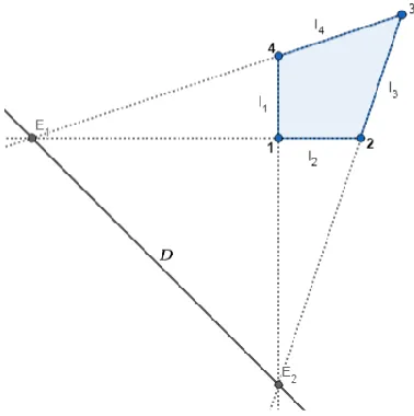
Let 𝑄 = (1,2, . . . , 𝑚), 𝑚 ≥ 4 be closed and convex polygon with m sides, in ℝ and 𝑖 ∈ ℤ be the verices of 𝑄 which are called nodes, where 𝑖 − 1 and 𝑖 are the consecutive nodes and ℤ denotes the set of integers under modulo m.

Let the Cartesian coordinates of the nodes 𝑖 − 1 and 𝑖 be (𝑥 , 𝑦 ) and (𝑥, 𝑦) respectively. Then, equation of the straight line passing through 𝑖 − 1 and 𝑖 is

𝑙(𝑥, 𝑦) = (𝑖 − 1, 𝑖) ≅ (𝑥 − 𝑥)(𝑦 − 𝑦) − (𝑦 − 𝑦)(𝑥 − 𝑥) = 0

Definition 1[21](see also[22

]) Sides of the polygon

Definition 2[19] Let 𝑠, 𝑖 ∈ ℤ be straight line passing through the nodes 𝑖 and 𝑖 − 1, referring relation (1), 𝑙 denotes the linear form of 𝑠.

Definition 3[21](see also[22])Wedge functions are the functions 𝑁: 𝑄 ⟶ ℝ of the form

𝑁(𝑥, 𝑦) = 𝐾 _{( , )}( , )(𝑖 ∈ ℤ ) (2)

where 𝐾 𝑠 are the normalizing constants.

Within the context of uniqueness, it is important to note that D(x,y) has a unique geometrical meaning for convex polygons. It is the equation of the straight line(see[21],[22]) connecting the exterior intersection points(cf. Fig. 1)

914 For the analysis of this paper, following properties of

wedge functions described in [21](see also[22]) for linear approximation over a polygonal element, have been considered:

Properties of wedge functions[21](see also[22]) The wedge functions are functions which are smooth within their associated element and posses the following properties: 1. There is a node at each vertex of the polygon. For each node there is an associated wedge within each polygon containing the node.

2. Wedge 𝑁(𝑥, 𝑦) associated with node i is normalized to unity at node i,

(𝑖 ∈ ℤ ).

3. Wedge 𝑁(𝑥, 𝑦) is linear on sides adjacent to i, (𝑖 ∈ ℤ ). 4. Wedge 𝑁(𝑥, 𝑦) vanishes on sides opposite to node i and at all nodes j for which 𝑗 ≠ 𝑖.

5. The wedges associated with 𝑄 form a basis for linear functions over it. For the polygon 𝑄 , there must be at least 𝑚 nodes. For these to suffice, one should have(cf. G.15 of [6]):

∑ ‍𝑁(𝑥, 𝑦) = 1 (3)

∑ ‍𝑥𝑁(𝑥, 𝑦) = 𝑥 (4)

∑ ‍𝑦𝑁(𝑥, 𝑦) = 𝑦 (5)

6. Each wedge function and all its derivatives are continuous within the polygon for which the wedge is a basis function.

The following concept of interpolation is also required for the analysis:

Definition 4 [16] Let W: W, W , . . . , W be a system of real valued functions on a set A, let 𝑥 , 𝑥 , . . . , 𝑥 be given distinct points of A and let 𝑐, 𝑐 , . . . , 𝑐 be given real numbers. The polynomial 𝑁(𝑥) = ∑ ‍𝑐𝑊 is said to interpolate the values 𝑐 if 𝑁(𝑥 ) = 𝑐 , 𝑘 = 1, . . . , 𝑛.

3 C

For a convex m-gon, a rational wedge function for degree k approximation, corresponding to the 𝑖 _{node has been} constructed as follows[21]:

𝑁 (𝑥, 𝑦) = _{( , )}( , ) (6)

where 𝑃( )_{(𝑥, 𝑦) is a polynomial of degree m, in x and y such} that it satisfies the wedge properties. For this, the numerator is the product of all the edges other than the ones which are adjacent to the given node, with the multiple of a constant 𝐾 to normalize it on the 𝑖 _{node(see [21], [22]). The denominator} of the wedge function is desired to be such that the wedge function remains a bi-variate polynomial of degree k on the adjacent sides.

3.1 Computation of denominator of the rational form of wedges

Using properties of wedge functions, now the denominator can be determined.

Referring relation (6), it is quite clear that in case of the quadrilateral element, numerator and denominator of 𝑁 𝑠

reduce to degree two and degree one respectively. In view of relation (3), the denominator is identically equal to the sum of the terms of the numerator. For the validity of this identity, it is mandatory to equate the coefficients of the terms of degree higher than one to zero. In this process, a system of three linear equations in four unknowns, 𝐾 ,( i=1,...,4) is obtained. Without loss of generality 𝐾(≠ 0) may be normalized to one.

Finally, a system of three equations in three unknowns 𝐾 , 𝐾 and 𝐾 , is left which can be expressed as

𝐀𝐊 = 𝐌 (7)

where A is a 3 × 3 matrix and K is the column vector ,𝐾 𝐾 𝐾- . As a first step, invertibility of the matrix A is established, to assure the existence and uniqueness of the solution of the system.

The value of 𝐾𝑠 thus obtained have been substituted in the left hand side of (3) to determine linear form of the denominator function.

3.2 Existence of the denominator function

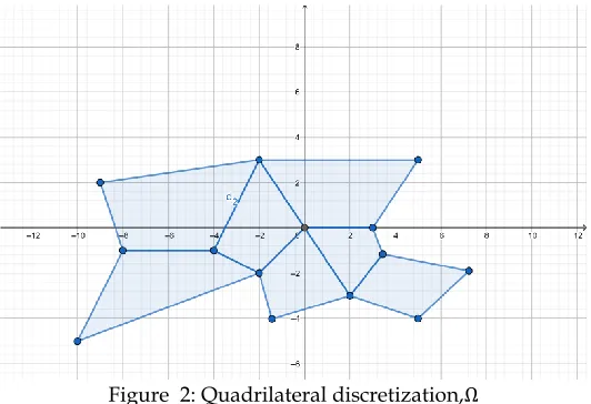
The main result, which establishes the existence and uniqueness of solution of the system of linear equations(7) under certain geometric constraints on the element under consideration, is proved in this part of the paper. Let Ω be the quadrilateral discretization of the domain ℝ (see Figure 2) and 𝑄 be an arbitrary quadrilateral element of Ω.

Figure 2: Quadrilateral discretization,Ω

Theorem 1 The denominator of the wedge functions corresponding to the element 𝑄 ∈ Ω exists and is unique if the following hold:

(a) No two opposite sides of 𝑄 are parallel. (b) No three vertices of 𝑄 are collinear.

Proof of Theorem 1

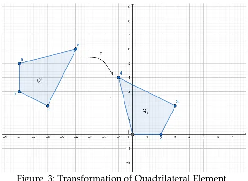
Figure 3: Transformation of Quadrilateral Element

By applying the transformations, viz. rotation and translation, the quadrilateral 𝑄 has been transformed into 𝑄 with vertices (1,2,3,4) having Cartesian coordinates (0,0), (𝑥, 0), (𝑥 , 𝑦 ) and (𝑥, 𝑦 ) respectively (cf. Figure 3). This transformation does not cause any loss to the generality.

Using notation of linear form described in (1), 𝑙 𝑠 (𝑖 = 1, . . ,4) have been computed

𝑙 = (4,1) ≅ 𝑥𝑦 − 𝑦𝑥 ‍,‍‍‍𝑙 = (1,2) ≅ 𝑦‍,‍‍‍𝑙 = (2,3) ≅ 𝑦 𝑥 − (𝑥 − 𝑥 )𝑦 − 𝑥 𝑦 ‍,‍‍‍

𝑙 = (3,4) ≅ (𝑦 − 𝑦)𝑥 − (𝑥 − 𝑥 )𝑦 − 𝑥 𝑦 +

𝑥 𝑦 (8)

The value of numerator of the wedge function 𝑁 corresponding to the 𝑖 _{node can be computed. In view of the} wedge properties, 𝑁 should vanish on the opposite sides of the node i and turns out to be linear on the adjacent sides. Denoting the numerator of 𝑁 by 𝑁𝑢𝑚, we have

𝑁𝑢𝑚 = 𝐾𝑙 𝑙 ‍,‍‍‍𝑁𝑢𝑚 = 𝐾𝑙 𝑙

𝑁𝑢𝑚 = 𝐾𝑙 𝑙 ‍,‍‍‍𝑁𝑢𝑚 = 𝐾𝑙 𝑙 (9)

Applying the technique, described in [8], consider ∑ ‍𝑁𝑢𝑚 and equate the coefficients of terms 𝑥𝑦 (𝑖 + 𝑗 = 2, i, j =0, 1, 2) to zero. Thus, the following system of three linear equations in three unknowns 𝐾 , 𝐾 and 𝐾 is obtained for 𝐾 = 1.

𝐾𝑦 𝑦 − 𝐾𝑦 = −(−𝑦 + 𝑦𝑦 ) (10)

−𝐾𝑥 + 𝐾𝑥 𝑥 − 𝐾𝑥 𝑥 + 𝐾𝑥𝑥 − 𝐾𝑥 += −(𝑥 𝑥 − 𝑥 − 𝑥 𝑥 + 𝑥 𝑥 )

−𝐾𝑥 𝑦 + 𝐾𝑥𝑦 − 𝐾𝑥𝑦 − 𝐾𝑥 𝑦 + 2𝐾𝑥 𝑦 = −(2𝑥 𝑦 − 𝑥 𝑦 + 𝑥 𝑦 −

𝑥𝑦 − 𝑥 𝑦 )

It may be verified easily that the coefficient matrix of the system (10) is invertible if

• 𝑦 ≠ 0 • 𝑦 ≠ 𝑦 • 𝑥 ≠ ( )

These conditions in turn imply assertions (a) and (b). Hence, the proof of Theorem 1 is completed Substituting the value of 𝐾𝑠, i=1,2,3,4, obtained on solving the system (10), the denominator of the wedge functions yields directly.

4 E

C

Algorithm of a program in Mathematica which supports the claim has been written here. In case of existence of the denominator function, it determines the wedge function. Further, it executes the task of computing approximant to the data provided and also generates the approximate surface. Algorithm illustrating this program is as follows:

Algorithm

Step1: :

Start

Step2: :

Declare variables n, 𝑥,4-, 𝑦,4-, nodes,4-, k,4-, R,3-,3-, K.

Step3:

Repeat steps until (𝑖 ≤ 4);𝑖 = 1. Let [ls(x,y)[𝑖]]=call function nodesToLines(nodes(x[𝑖],y[𝑖]),x,y). Step4:

Repeat steps until (𝑖 ≤ 4);𝑖 = 1. m:=Mod[i+2,4];

If [m==0, num[i]:= k[[i]]*ls[[i+2]]*ls[[1]], num[i]:=k[[i]]*ls[[m]]*ls[[m+1]]]

Step5: : Let deno(x,y)=deno(x,y)+call

Expand([num(x,y),[𝑖]]);𝑖 = 1; 𝑖 ≤ 4.

Step6: : Let L={call Coefficient(deno(x,y), pow(x,2)), call Coefficient(deno(x,y), pow(y,2)),

call Coefficient(deno(x,y), pow(x*y,1))}.

Step7:

Repeat 𝑖=1,𝑖 ≤ 3. Repeat 𝑗=2, 𝑖 ≤ 4.

R[𝑖][𝑗]=call Coefficient(k[𝑗] in L[[𝑖]]).

Step 8:

If call Det(R)=0 then exit.

Else

Call function Solve for L[[i]], i=1 to 3 equated to 0 with respect to 𝑘 , 𝑘 , 𝑘 .

Repeat until 𝑖 ≤ 4; 𝑖=1.

Let ,𝑁(𝑥, 𝑦), ,𝑖-- = ,𝑛𝑢𝑚(𝑥, 𝑦), ,𝑖--/𝑑𝑒𝑛𝑜(𝑥, 𝑦). Input function f(x,y), to be approximated.

Repeat until 𝑖 ≤ 4; 𝑖=1. a[𝑖]=f(nodes(x[𝑖],y[𝑖])]). The approximant Ap(x,y)=Ap(x,y)+call Expand(a[𝑖]*N[𝑖](x,y));𝑖 = 1;𝑖 ≤ 4.

Plot Ap(x,y) and f(x,y) over the considered quadrilateral.

Step9: : Stop.

916 User defined functions

Intercept

:

𝐼𝑛𝑡𝑒𝑟𝑐𝑒𝑝𝑡‍((𝑥, 𝑦 ), (𝑥 , 𝑦 )) = (𝑦 − 𝑦, 𝑥 − 𝑥 , −𝑥 ∗ 𝑦 + 𝑦 ∗ 𝑥 )

nodesToIntercepts 𝑛𝑜𝑑𝑒𝑠𝑇𝑜𝐼𝑛𝑡𝑒𝑟𝑐𝑒𝑝𝑡𝑠(𝑝)= 𝐼𝑛𝑡𝑒𝑟𝑐𝑒𝑝𝑡𝑠(𝑝, 𝑅𝑜𝑡𝑎𝑡𝑒𝑅𝑖𝑔𝑕𝑡(𝑝)):

nodesToLines :

nodesToLines(p,(x,y))=-Dot(nodesToIntercept(p),(x,y,1)) ls 𝑙𝑠 = 𝑛𝑜𝑑𝑒𝑠𝑇𝑜𝐿𝑖𝑛𝑒𝑠(𝑛𝑜𝑑𝑒𝑠, (𝑥, 𝑦)):

5 Numerical Examples

In support of the assertions of this paper, following numerical examples have been illustrated:

Example 1(When assertions (a) and (b) are true) Consider the quadrilateral 𝑄 = (1,2,3,4) with Cartesian coordinates of the vertices as (cf. Figure4) 1=(0,0), 2=(2,0), 3=(1.5,1) and 4=(0.5,0.75). Then, referring relation(7) the matrix A will be

Figure 4: Quadrilateral Element

𝐴 =

[ −7

8 3

2 −2

1

2 −1 −1

3

16 0 0 ]

,

Clearly, determinant of A is nonzero. Hence, the denominator function D(x,y) exists uniquely and

𝐷(𝑥, 𝑦) = (8𝑥 − 17𝑦 + 20) the wedge function 𝑁, corresponding to the 𝑖 _{node, (𝑖 =} 1,2,3,4) will be:

𝑁 = − 𝑁 = _{( )} 𝑁 =

𝑁 = − ( _{( )} )

Case 1 Let 𝑓(𝑥, 𝑦) = 2𝑥 + 𝑦 is to be approximated, it may be verified easily that the resulting approximant is f(x,y) itself.

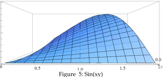
Case 2 If any non linear function is to be approximated, say 𝑓(𝑥, 𝑦) = 𝑠𝑖𝑛(𝑥𝑦) then the approximant is 𝜙(𝑥, 𝑦)(𝑠𝑎𝑦) = , - , -

( ) . Figure 5, represents f(x,y) over the element 𝑄 and its approximation is displayed in Figure 6.

Figure 5: Sin(xy)

Figure 6: Approximant to Sin(xy)

Example 2 (When assertions (a) and (b) of Theorem 1 are violated) Consider the quadrilateral 𝑄 = (1,2,3,4) such that 1=(0,0), 2=(2,0), 3=(1,1) and 4=(0.5,1) (cf Figure 7).

Figure 7: Element with parallel sides

Then, the matrix A(cf. relation (7)) will be

𝐴 =

[ −1

2 2 −2

1

4 −1 −2

0 0 0 ]

Since |𝐴| = 0, obviously the matrix is not invertible and thus, the denominator function D(x,y) does not exist uniquely.

6 C

Dasgupta‘s contribution in computing the wedge functions makes the process more viable to be solved using computers, as it sets the method free from geometry. From application point of view, it may be noted that this approach is more preferable than previous ones. Moreover, it may be easily implemented by using software based on Mathematics, in particular Mathematica. Identifying the conditions of existence and uniqueness of the wedge functions makes the process more plausible.

A

A

Example of a Quadrilateral:Mathematica program implementing the algorithm in section 4

n = 4;

(*Coordinates of the vertices*) xy = {{0, 2, 3/2, 1/2}, {0, 0, 1, 3/4}}

nodes = Transpose[xy]

(*Linear forms*)

Intercept[{x1_, y1_}, {x2_, y2_}] := {y2 - y1, x1 - x2, -x1*y2 + y1*x2}

nodesToIntercepts[p_?MatrixQ]:= Thread[Intercept[p, RotateRight[p]]]

nodesToLines[p_,{x_,y_}]:=-Dot[nodesToIntercepts[p], {x, y,1}]

ls = nodesToLines[nodes, {x, y}]

(*Figure representing the quadrilateral*) Graphics[Polygon[nodes]]

(*Weights*) k = {k1, k2, k3, k4};

(*Construction of wedge functions*)

For[i = 1, i < 5, i++, m := Mod[i + 2, 4];

If[m == 0,

num[i] := k[[i]]*ls[[i + 2]]*ls[[1]], num[i] := k[[i]]*ls[[m]]*ls[[m + 1]] ]

]

deno = Expand[Sum[num[i], {i, 1, 4}]]

L={Coefficient[deno,x,2],Coefficient[deno,y,2],Coefficient[den o, x*y, 1]}

ClearAll[R]

R:=({{Coefficient[L[1], k2], Coefficient[L[1], k3], Coefficient[L[1], k4]},{Coefficient[L[2],k2],Coefficient[L[2],k3], Coefficient[L[2], k4]},{Coefficient[L[3], k2], Coefficient[L[3], k3], Coefficient[L[3], k4]}})

K := Det[R]

(*verification of the condition of existence*)

If[K == 0, NotebookClose[], Print[Entries are valid]]

k1 := 1;

Table[L[[i]] == 0, {i, 3}];

Solve[%, {k2, k3, k4}] For[i = 1, i < 5, i++,

(𝑆𝑢𝑏𝑠𝑐𝑟𝑖𝑝𝑡,𝑁, 𝑖-)[{x, y}] = Thread[Expand[num[i]]/deno] /. %]

ClearAll[f, x, y];

(*Function to be approximated*)

𝑓,*𝑥_, 𝑦_+- = 𝑆𝑖𝑛,𝑥 ∗

𝑦-For[i = 1, i < 5, i++, a[i] = f[nodes[[i]]]] ClearAll[A1];

(*Approximant*) A1=

Thread[ApartThread[Apart[Sum[a[i]*(𝑆𝑢𝑏𝑠𝑐𝑟𝑖𝑝𝑡,𝑁, 𝑖-)[{x, y}], {i, 1, 4}]]]

(*Plot of the approximant*)

Plot3D[A1, {x, 0, 2}, {y, 0, 1}, 𝑉𝑖𝑒𝑤𝑃𝑜𝑖𝑛𝑡 ⟶ Front, 𝑅𝑒𝑔𝑖𝑜𝑛𝐹𝑢𝑛𝑐𝑡𝑖𝑜𝑛 ⟶ 𝐹𝑢𝑛𝑐𝑡𝑖𝑜𝑛,*𝑥, 𝑦+, 𝑙𝑠,,1-- ≤ 0&&𝑙𝑠,,2-- ≤ 0 &&𝑙𝑠,,3-- ≤ 0&&𝑙𝑠,,4-- ≤

0--R

[1] D. Apprato, R. Arcangeli and J. L. Gout, Rational interpolation of Wachspress error estimates, Comp. and Maths.with Appls, Pargamon Press Ltd vol 5, 329-336, 1979.

[2] J. H. Argyris, and S. Kelsey, Energy Theorems and Structural Analysis, Butterworths, London, 1960.

[3] R. W. Clough and P. Joseph, "Dynamics of Structures", Computers and Structures, Inc.,2003.

[4] R. W. Clough, The Finite Element Method in Plane Stress Analysis, American Society of Civil Engineers,345-378, 1960.

[5] R. Courant, Variational Methods for the Solution of Problems of Equilibrium and Variations, Bulletin of the American Mathematical Society, vol 49, 1-23, 1943. [6] G. Dasgupta, ―Finite Element Concepts: A Closed Form

Algebraic Development‖, Springer, New York, 2018. [7] G. Dasgupta and E. L. Wachspress, The adjoint for an

algebraic finite element. Comput. Math. Appl. vol 55, 1988–1997, 2008.

[8] G. Dasgupta, ‖Interpolants within convex polygons: Wachspress‘ Shape Functions‖, Journal of Aerospace Engineering, Vol. 16, No. 1,1-8, 2003.

[9] M. S. Floater, Mean-value coordinates. Comput. Aided Geom. Des., vol 20, 19–27, 2003.

[10]∅ Hjelle, M. Dæhlen, Triangulations and Applications, Springer-Verlag Berlin Heidelberg, 2006.

[11]A. Hrennikoff, Solution of Problems in Elasticity by the Frame Work Method, Journal of Applied Mathematics, Vol. 8, No. 4, 169-175, 1941.

[12]D. Levin, Multidimensional Reconstruction by Set-valued Approximations, IMA Journal of Numerical Analysis, vol 6, 173-184, 1986.

[13]S. Levy, Structural Analysis and Influence Coefficients for Delta Wings, Journal of Aeronautical Sciences, vol. 20, no. 7, pp. 449-454, July 1953.

547-918 560, 1947.

[15]P. Lidberg, Barycentric and Wachspress coordinates in two dimensions: theory and implementation for shape transformations. Technical Report U.U.D.M. Project Report 2011:3, Uppsala Universitet, 2011.

[16]G. G. Lorentz, Approximation of Functions, Holt, Tinehart and Wilson, U.S.A., 1966.

[17]D. McHenry, ―A Lattice Analogy for the Solution of Plane Stress Problems,‖ Journal of Institution of Civil Engineers, Vol. 21, 59-82, 1943.

[18]A. F. Mobius, Der Barycentrische Calcul, Johann Ambrosius Barth, Leipzig, 1827.

[19]P. L. Powar, S. S. Rana, Construction of ‗Wachspress type‘ rational basis functions over rectangles, Proc. Indian Acad, Sci.(Math. Sci.), vol 110, no. 1, 69-77, February 2000. [20]M. J. Turner, R. W. Clough, H. C. Martin and L. J. Topp, Stiffness and Deflection Analysis of Complex Structures, Journal of the Aeronautical Sciences, vol 23, 805-823, 1956. [21]E. L. Wachspress ―Rational Bases and Generalized Barycentrics: Applications to Finite Elements and Graphics‖, Springer, New York, 2015.