https://doi.org/10.5194/esd-9-969-2018
© Author(s) 2018. This work is distributed under the Creative Commons Attribution 4.0 License.
Using network theory and machine learning
to predict El Niño
Peter D. Nooteboom1,3, Qing Yi Feng1,3, Cristóbal López2, Emilio Hernández-García2, and Henk A. Dijkstra1,3
1Institute for Marine and Atmospheric Research Utrecht (IMAU), Department of Physics,
Utrecht University, Utrecht, the Netherlands
2Instituto de Física Interdisciplinar y Sistemas Complejos (IFISC, CSIC-UIB), University of the Balearic
Islands, Balearic Islands, Spain
3Centre for Complex Systems Studies, Utrecht University, Utrecht, the Netherlands
Correspondence:Peter D. Nooteboom ([email protected])
Received: 7 March 2018 – Discussion started: 13 March 2018 Revised: 22 June 2018 – Accepted: 26 June 2018 – Published: 23 July 2018
Abstract. The skill of current predictions of the warm phase of the El Niño Southern Oscillation (ENSO) reduces significantly beyond a lag time of 6 months. In this paper, we aim to increase this prediction skill at lag times of up to 1 year. The new method combines a classical autoregressive integrated moving average technique with a modern machine learning approach (through an artificial neural network). The attributes in such a neural network are derived from knowledge of physical processes and topological properties of climate networks, and they are tested using a Zebiak–Cane-type model and observations. For predictions up to 6 months ahead, the results of the hybrid model give a slightly better skill than the CFSv2 ensemble prediction by the National Centers for Environmental Prediction (NCEP). Interestingly, results for a 12-month lead time prediction have a similar skill as the shorter lead time predictions.
1 Introduction
Approximately every 4 years, the sea surface temperature (SST) is higher than average in the eastern equatorial Pacific (Philander, 1990). This phenomenon is called an El Niño and is caused by a large-scale ocean–atmosphere interac-tion between the equatorial Pacific and the global atmosphere (Bjerknes, 1969), referred to as the El Niño Southern Oscil-lation (ENSO). It is the dominant mode of climate variability at interannual timescales and has teleconnections worldwide. As El Niño events cause enormous damage worldwide, skill-ful predictions, preferable for lead times up to 1 year, are highly desired.
So far, both statistical and dynamical models are used to predict ENSO (Chen et al., 2004; Yeh et al., 2009; Fedorov et al., 2003). However, El Niño events are not predicted well enough up to 6 months ahead due to the existence of the so-called predictability barrier (Goddard et al., 2001). Some the-ories indicate that this is due to the chaotic, yet
determinis-tic, behaviour of the coupled atmosphere–ocean system (Jin et al., 1994; Tziperman et al., 1994). Others point out the importance of atmospheric noise, acting as a high-frequency forcing sustaining a damped oscillation (Moore and Klee-man, 1999).
Recently, attempts have been made to improve the ENSO prediction skill beyond this spring predictability boundary, for example by using machine learning (ML; Wu et al., 2006) methods, also combined with network techniques (Feng et al., 2016). ML has shown to be a promising tool in other branches of physics, outperforming conventional methods (Hush, 2017). As the amount of data in the climate sciences is increasing, ML methods such as artificial neural networks (ANNs), are becoming more interesting to apply to predic-tion studies.
has to choose how large and complicated the ANN struc-ture is. The more complicated an ANN, the more it will fil-ter the important information from the attributes itself, but it will require more input data and is computationally inten-sive. Therefore, simpler ANN structures are used in this arti-cle. However, techniques will have to be applied in order to reduce the amount of input variables and select the important ones, to make the problem appropriate for the simpler ANN. This reduction and selection problem can be tackled in many ways, which are crucial for the prediction. The main issue in these methods, however, is what attributes to use for ENSO prediction.
Complex networks turn out to be an efficient way to rep-resent spatiotemporal information in climate systems (Tso-nis et al., 2006; Steinhaeuser et al., 2012; Fountalis et al., 2015) and can be used as an attribute reduction technique. These climate networks are in general constructed by linking spatiotemporal locations that are significantly correlated with each other according to some measure. It has been demon-strated that relationships exist between topological properties of climate networks and nontrivial properties of the under-lying dynamical system (Deza et al., 2014; Stolbova et al., 2014), also specifically for ENSO (Gozolchiani et al., 2011, 2008; Wang et al., 2015). Climate networks already appear to be a useful tool for more qualitative ENSO prediction, by considering a warning of the onset of El Niño when a cer-tain network property exceeds some critical value (Ludescher et al., 2014; Meng et al., 2017; Rodríguez-Méndez et al., 2016).
In this paper, a hybrid model is introduced for ENSO prediction. The model combines the classical linear statis-tical method of autoregressive integrated moving average (ARIMA) and an ANN method. ANN is applied to predict the residual, due to the nonlinear processes, that is left af-ter the ARIMA forecast (Wu et al., 2006). To motivate our choice for attributes in the ANN, we use an intermediate-complexity model which can adequately simulate ENSO be-haviour, the Zebiak–Cane (ZC) model (Zebiak and Cane, 1987). The attributes which are used in the prediction model are related to physical processes which are relevant for ENSO prediction. Moreover, network variables are consid-ered as attributes such that they relate to a physical mecha-nism, but additionally contain spatial information.
Section 2 briefly describes the ZC model, the methods considering both the climate networks and ML, and the data from observations. In Sect. 3, the network methods are first applied to the ZC model. Second, the attributes selected for observations are presented. These attributes, among which there is a network variable, are applied in the hybrid predic-tion model in Sect. 4, which discusses the skill of this model to predict El Niño. The paper concludes with a summary and discussion in Sect. 5.
2 Observational data, models and methods
2.1 Data from observations
As observational data, we use the sea surface height (SSH) from the weekly ORAP5.0 (Ocean ReAnalysis Pilot 5.0) re-analysed dataset of ECMWF from 1979 to 2014 between 140 to 280◦E and 20◦S to 20◦N.
For recent predictions, the SSALTO/DUACS altimeter products are used for the same spatial domain, since the SSH is available from 1993 up to the present in this dataset. The SSALTO/DUACS altimeter products were produced and dis-tributed by the Copernicus Marine and Environment Moni-toring Service (http://marine.copernicus.eu/, June 2017).
In addition, the HadISST dataset of the Hadley Centre has been used for the SST and the NCEP/NCAR Reanalysis dataset for the wind stress from 1980 to the present (Rayner et al., 2003).
To quantify ENSO, the NINO3.4 index is used, i.e. the 3-month running mean of the average SST anomaly in the extended reconstructed SST dataset between 170 to 120◦W and 5◦S and 5◦N (Huang et al., 2015).
The warm water volume (WWV), being the integrated volume above the 20◦C isotherm between 5◦N–5◦S and 120–280◦E, is determined from the temperature analyses of the Bureau National Operations Centre (https://www. pmel.noaa.gov/elnino/upper-ocean-heat-content-and-enso, National Oceanic and Atmospheric Administration, 2017).
2.2 The Zebiak–Cane model
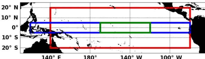
The ZC model Zebiak and Cane (1987) represents the cou-pled ocean–atmosphere system on an equatorialβ-plane in the equatorial Pacific (see Fig. 1). This model is used here to infer which processes are important for ENSO prediction and to find the attributes which represent those processes. Also, a network analyses is applied to the ZC model in order to find network variables which could improve prediction, before these network variables are calculated in observations. We use the numerically implicit version of this model (van der Vaart et al., 2000; von der Heydt et al., 2011) as in Feng (2015).
Figure 1.Pacific area (red rectangle) from 140–280◦E to 20◦S–20◦N, the NINO3.4 area (green rectangle) from 170–120◦W to 5◦S–5◦N and the WWV area (blue rectangle) from 120–280◦E to 5◦S–5◦N.
As shown in van der Vaart et al. (2000), the parameter measuring the magnitude of the ocean–atmosphere coupled processes is the coupling strength µ. Without any included noise, a temperature anomaly damps out to a constant value and a stationary state ifµ < µc, whereµcindicates a critical value. However, if the coupling strength exceeds the critical valueµc, a supercritical Hopf bifurcation occurs. A perturba-tion then does not decay, but an oscillaperturba-tion is sustained with a period of approximately 4 years.
Three positive feedbacks related to the thermocline depth, upwelling and zonal advection can cause the amplification of SST anomalies (Dijkstra, 2006), while the oscillatory be-haviour associated with ENSO is caused by negative delayed feedbacks. The “classical delayed oscillator” paradigm as-sumes this negative feedback is caused by waves through geostrophic adjustment, controlling the thermocline depth. A complementary, different view is the “recharge/discharge os-cillator” (Jin, 1997), also regarding oceanic waves excited through oceanic adjustment. The waves excited to preserve the Sverdrup balance are responsible for a transport of warm surface water to higher latitudes, discharging the warm wa-ter in the tropical Pacific. The thermocline depth is raised, resulting in more cooling of SST. The WWV is the variable generally used to capture how much the tropical Pacific is “charged”.
Apart from the coupled ocean–atmosphere processes, ENSO is also affected by fast processes in the atmosphere, which are considered as noise in the ZC model. An impor-tant example of atmospheric noise are the so-called westerly wind bursts (WWB). These are related to the Madden–Julian oscillation (Madden and Julian, 1994). The WWB is a strong westerly anomaly in the zonal wind field, occurring every 40 to 50 days and lasting approximately 1 week. The ef-fect of the noise on the model behaviour depends on whether the model is in the super- or subcritical regime (i.e. whether µ is above or belowµc). If µ < µc, the noise excites the ENSO mode, causing irregular oscillations. In the supercrit-ical regime, a cycle of approximately 4 years is present, and noise causes a larger amplitude of ENSO variability.
The atmospheric noise in the model is represented by ob-taining a residual of the wind stress from observations as in
Feng and Dijkstra (2016). Since weekly data are considered, every discrete time step in the model is 1 week.
2.3 Network variables
Here we explain the methods to calculate a property of a cli-mate network which is tested in the ZC model and observa-tions and will be used in the hybrid model. From the network analysis we found several climate network quantities with in-teresting properties for prediction, but which are not used in the hybrid model of the next section. The methods to calcu-late these properties can be found in Appendix A1.
An undirected and unweighted network is constructed making use of the Pearson correlation of climate variables related to ENSO (e.g. SST, thermocline depth or zonal wind stress). Network nodes are model or observation grid posi-tionsiand the links are stored in a symmetric adjacency ma-trixA, whereAij=1 if node iis connected to nodej and Aij=0 otherwise.Aij is defined by
Aij=2
Rij
−
−
δij. (1)
HereRij is the Pearson correlation between nodei andj, is the threshold value and2denotes the Heaviside func-tion. Hence, if the Pearson correlation exceeds the threshold , the two nodes will be linked. Theδijis the Kronecker delta function, implemented to prevent connection of nodes with themselves.
Percolation theory is then considered, describing the con-nectivity of different clusters in a network. It has been found that the connectivity of some climate networks increases just before an El Niño and decreases afterwards (Rodríguez-Méndez et al., 2016), as local correlations between points increase and decrease. At such a percolation-like transition, the addition of only a few links can cause a considerable part of the network to become connected. Before the percolation transition, clusters of small sizes will form. Therefore the variablecswill warn for the transition:
cs=sns
N . (2)
fraction of nodes that are part of a cluster of (generally small) sizes.
2.4 Hybrid prediction model
A hybrid model (Valenzuela et al., 2008) will be applied to predict ENSO, in which the observationZt at timet is rep-resented by
Zt=Yt+Nt. (3)
Here Yt is modelled by a linear process andNt by a ML-type technique. Let eYt be the prediction of the part Yt us-ing ARIMA, thenZt−eYt is the residual with respect to the observed value. This residual will be predicted by the feed-forward ANN:
e
Nt=f(x1(t),· · ·, xN(t)). (4)
Here f is a nonlinear function of the N attributes x1(t),· · ·, xN(t) andNet the prediction of residualZt−Yet at timet. Notice the nonlinear functionf does not depend on history, whereas the ARIMA parteY does. The final
predic-tionZte of the hybrid model is
e
Zt=eYt+Nte. (5)
Previous work showed that the results of a hybrid model are in general more stable and reduce the risk of a bad predic-tion, compared to a single prediction method (Hibon and Ev-geniou, 2005). “More stable” means that a hybrid model has a lower variability in prediction skill for different arbitrary time series. Besides, ARIMA is a simple method to include information about the history in the prediction model, which is not in the feed-forward ANN.
This scheme describes a “supervised” model, implying that the predictant is “known”. This known quantity is the NINO3.4 index. The standard procedure for supervised learning is to optimize the ML method on a “training set” to define an optimal model, which predicts ENSO with a cer-tain time ahead. This function will then be tested on a test set. Here a training set of 80 % and a test set of 20 % of the total time series is used. The dataset can be represented by aT×N matrix, whereT represents the length of the time series and each timet=1,···, T has a set ofNattributesx1(t),···, xN(t).
Note that, since we are predicting time series, for any training set[titrain, tftrain]and test set[titest, tftest],titest> tftrainis
conve-nient (wheretitrain, tftrain, titest, tftest∈ [1, T]). In the following, we describe more in detail the different parts of this hybrid prediction method.
First, the training set is used to optimize an ARIMA(p, d, q) process for the NINO3.4 time series. The standard method maximizing the log likelihood function is used to fit α1,· · ·, αp, β1,· · ·, βq, such that Ptε2t is
minimized for time seriesZt withtin months:
1−α1B−···−αpBp(1−B)dZt
= 1+β1B+···+βqBq
εt, (6)
whereεt is the residual, differencing orderd determines the amount of differencing terms, p is the amount of autore-gressive terms andqis the amount of moving average terms on the right-hand side;B (BZt=Zt−1) is the lag operator.
Finding the most optimal ARIMA order (p, d, q) is not trivial (Zhang, 2003; Aladag et al., 2009). General methods include the Akaike’s information criterion (Akaike, 1974) or min-imum description length (Rissanen, 1978). However, these methods are often not satisfactory and additional methods have been proposed to determine the order (Al-Smadi and Al-Zaben, 2005). In this article we mainly present results ob-tained with ordersp=12,d=1 andq=0 orq=1, which gave good prediction skill and it can be argued that in such a chaotic system, information from too long ago is not impor-tant anymore.
The eventual ARIMA equation results in a prediction
ˆ
Yt(Zt−1,···, Zt−p, εt−1,···, εt−q) ofτ =1 months ahead. Here εt−1=Zt−1− ˆYt−1. Let eYt be the ARIMA prediction of τ >0 months ahead, by calculatingYˆt forτ times in the fu-ture and replacing any observationZt with the consecutive calculatedYˆt, wheret is in the future and Zt therefore un-known. Similarly, ifq=1 andτ >1 months, the residual is calculated byt−1=eYt−1− ˆYt−1, since the observed value
Zt−1is in the future. Hence the ARIMA prediction eYt will
be a time extrapolation with the optimized ARIMA model. AftereYt is predicted by the ARIMA model, the ANN will
be used for the predictionNte, making use of more variables
than the NINO3.4 index alone. Deciding which of the vari-ables to use is not a straightforward problem, yet crucial for the eventual prediction. Generally in an ANN, a pair of two variables can be compatible in the prediction, but per-form poor when applied alone. Other pairs can be redundant and cover important information when used alone, but solely noise is included when used together (Guyon and Elisseeff, 2003). Adding a variable to the attribute set and seeing if it improves prediction can only conclude whether it improves prediction with respect to the old attribute set, not whether the variable is predictive in itself. To determine the attribute set, we consider which variables represent a certain physical mechanism that is important for the ENSO prediction. This helps to find attributes which are not related to each other, but include important information on their own. Besides, it is tested whether the prediction skill is reduced if a variable is dropped out of the attribute set.
cor-relation between the predictor and predictant is a commonly used measure for attribute selection (Hall, 1999). Therefore the Pearson cross-correlation is calculated for the attributes at lagτ to show the predictability of a time series:
Rτ(p, q)=max τ
Pn
k=1p(tk)q(tk−τ)
q Pn
k=1p2(tk)
Pn
k=1q2(tk−τ)
. (7)
Here p is the predictor, q is the predictant and lagτ≤64 weeks such that no information too far in the past is consid-ered.
However, the effect of a variable on ENSO at a short lead time increases the cross-correlation at a longer lead time, due to the effect of autocorrelation (Runge, 2014). To solve this autocorrelation problem, a Wiener–Granger causality F test (Sun et al., 2014) is performed between all predictors x1,· · ·, xNand the predictant at lagsτ. Note Granger causal-ity is not the same as a “true” causalcausal-ity. If the test results in a lowp value, the null hypothesis thatxi does not cause in the Granger sense the predictant, due to Granger causality, is rejected at a low significance level (i.e.xi is more likely to cause the predictant due to Granger causality). Notice that both the cross-correlation and Wiener–Granger method give us merely an idea of which variables can be used for the pre-diction at different lead times. Both methods are linear, while the attributes will be used in a nonlinear method.
Finally, theT×Ndataset with selected attributes is used to predict the residual between the ARIMA forecast and the ob-servations in an ANN. Besides using the NINO3.4 sequence itself, the additional attributes can be applied to add impor-tant information and improve the prediction.
In this paper, only a feed-forward ANN is applied, hav-ing a structure without loops. The input variables are linearly combined and projected to the first layer neurons according to (Bishop, 2006):
zj=h D
X
i=1
wj i(1)xi+w(1)j0
!
. (8)
Herezjis the value of thejth neuron of the layer;wj i(1)is the weight between input xi from neuronito neuron j, where the (1) denotes the first layer.w(1)j0 is referred to as the bias.h is the sigmoid activation function, essential for incorporating the nonlinearity in the prediction model.
These zj can again be used as input for a second layer, which can be used for a third layer, and so on. Eventually this leads to some output which can be compared with the time series that must be predicted. Using a backward-propagating technique, the squared errorP
t(yt− ˆyt)2between the resid-ual we are predictingyt and the output of the ANNyˆt will be minimized over the weights for the training set. The op-timized function can then be tested on the test set. Initially, some random distribution of weights is used. The ANN part of the prediction will be performed with the toolbox Climate-Learn (Feng et al., 2016).
To summarize the tuning of the hybrid model: the ARIMA order and the hyperparameters controlling the ANN struc-ture are tuned on the data, i.e. such that the prediction result is optimal. However, we will consider whether some set of different parameter values converges to similar predictions, which can show whether the hyperparameter tuning was a one lucky shot or not. The choice of the attributes is based on the ZC model giving a more physical basis for the infor-mation needed for a good prediction. To select them at a spe-cific lag their cross-correlation and Wiener–Granger causal-ity with the ENSO index and performance are also consid-ered, which could lead to the replacement of an attribute with another attribute which is physically related.
3 Analysis of network properties and selection of ML attributes
In this section, topological properties of climate networks are analysed within the ZC model and observations, which lead to specific choices of attributes in the hybrid prediction model.
3.1 Network variables from the ZC model
Weekly spatiotemporal data on a 31×30 grid in the Pacific region are obtained for 45 years from the ZC model, to con-struct the climate networks. The first 5 years are not consid-ered, to discard the effect of the initial conditions. A sliding-window approach is used to calculate the network variables. This implies that a different network is calculated at each time, which is sliding 4 weeks ahead every time step. For the ZC model, either the thermocline network (fromh), SST net-work (fromT), wind-stress network (fromτx) or a combina-tion of these are considered for network construccombina-tion. Only the network variable which showed the same behaviour in the observations and in the ZC model is presented here. Other network variables with interesting properties can be found in Appendix A2.
The network variable of interest isc2 (the proportion of nodes belonging to clusters of size two) of the thermocline network, because it indicates the approach to a percolation transition of the network during an El Niño event (Fig. 2). A window of 1 year is used.c2 increases approximately 1 to 2 years before an El Niño event. This is mainly clear in the supercritical case. In the subcritical case, a clear warning of an event occurs when the oscillation of ENSO is more clear and the El Niños are stronger. Becausec2is a warning signal of an El Niño event in the ZC model, we will look in the next section at how it behaves when it is calculated from observations.
3.2 Selecting attributes from observations
Figure 2.The network variablec2of the thermocline network with a sliding window of 1 year in red and NINO3.4 in black in the ZC model.
(a)The subcritical (µ=2.7) case with threshold=0.99999 and(b)the supercritical (µ=3.25) case with=0.999.
Figure 3.The WWV,c2and the NINO3.4 index from observations for(a)the whole considered time series and (b)only during the 1997 El Niño. A warning of the El Niño event is visible for the WWV and c2.c2 gives a warning almost a year before the 1997 El Niño, while the WWV warns almost 7 months ahead.
to predict El Niño. Although the network variables show in-teresting behaviour in the ZC model for prediction, this is not always the case in observations. This section describes which variables, including a network variable, are implemented in the hybrid model and the selection of these attributes at dif-ferent lead times. Notice that only anomalies of the time se-ries in observations are considered.
First, from the recharge/discharge oscillator point of view, the WWV shows great potential for the prediction of ENSO (Bosc and Delcroix, 2008; Bunge and Clarke, 2014). There-fore it is used in the attribute set. The second attribute is a net-work variable related to WWV. The correlations of the SSH time series on a grid of 27 latitude points and 30 longitude points in the Pacific area are used to reconstruct a network with a threshold=0.9 and a sliding window of 1 year. The SSH is used instead of thermocline depth, because more data is available and it is by approximation proportional to the thermocline depth (Rebert et al., 1985). During an El Niño event, the link density of this network increases in the warm pool and the cold tongue specifically, causing a percolation-like transition. As discussed in the previous section, an early warning could be obtained withc2. This variable allows us
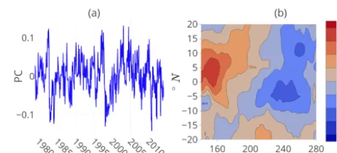
Figure 4.(a)The second principal component of the residual of the wind stress (PC2) and(b)its EOF, associated with the WWBs.
to extend the lead time of the WWV (Fig. 3). Third, atmo-spheric noise from the WWBs are a limitation for the pre-diction of ENSO (Moore and Kleeman, 1999; Latif et al., 1988). To obtain a variable related to the WWBs, the linear effect of the SST is subtracted from the zonal component of the wind stress. The second principal component (PC2), ex-plaining 8 % of the variance, is associated with these WWBs. In Fig. 4, the principal component and its empirical orthog-onal function (EOF) are presented. The peaks in the princi-pal component are visible before the great El Niño events of 1982 and 1997. Thereby, the EOF has the typical WWB structure, being positive west from the dateline and negative east. Finally, the attribute set does not yet contain any infor-mation about the seasonal cycle (SC) yet. The phase locking of an El Niño event to boreal winter is very typical to ENSO. Therefore a sinusoid with a period of 1 year is used as at-tribute, to see if it can improve the prediction skill.
Figure 5.(a)The cross-correlation of the PC2, WWV andc2with respect to NINO3.4 for different lags τ. (b) Thep value of the Wiener–Granger hypothesis test for the same lags. A lowpvalue implies the variable is likely to cause the NINO3.4 index at the spe-cific lag due to Granger causality. The p values of the PC2and WWV are almost zero for all lags.
Granger test has a local minimum close to a lag of 44 weeks. According to these methods,c2is especially predictive at the longer lead times close to 44 weeks.
To summarize, we are interested in the variables that repre-sent specific physical characteristics related to the prediction of ENSO, to select the attributes. Bothc2and the WWV are related to the recharge/discharge mechanism. PC2is related to the atmospheric noise from WWBs. The SC is related to the phase locking of El Niño events to boreal winter. The hybrid model allows us to implement different variables in the attribute set at different lead times. Therefore, the cross-correlations and Wiener–Granger causality were used to de-termine which attribute is more optimal at various lead times. This showed that it is better to usec2instead of WWV at lead times of more than 40 weeks. The other network variables which were interesting for the ZC model output (see the Ap-pendix) are performing worse when applied to observations and hence are not used as attributes in the hybrid model.
4 Prediction results
This section presents the predictions of the hybrid model, as compared with observations and with alternative predic-tions from the CFSv2 model ensemble of NCEP. The skill with ANN structures up to three hidden layers is investi-gated. First, a comparison between both predictions is made for the year 2010 (Fig. 6). Moreover, several lead time pre-dictions are shown and compared to the available CFSv2 lead time predictions. Next it is shown that these prediction mod-els converge to similar results for different hyperparameters and when using different training and test sets in a cross-validation method. Finally, a recent forecast is made and it is shown how the hybrid model predicts the development of ENSO the coming year.
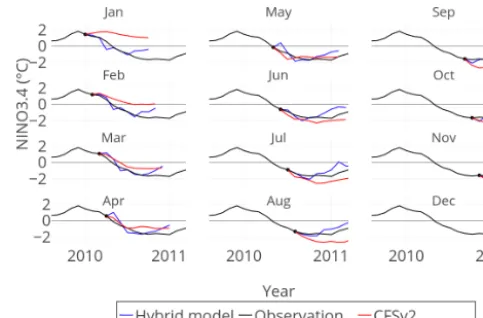
Figure 6. The 9-month ahead prediction starting from every month in the year 2010. Blue is the hybrid model prediction with ARIMA(12,1,1), 2×1×1 ANN structure and attributes are the 3-month running mean of WWV, PC2and SC. The black line is the observed index. Red is the mean of the CFSv2 ensemble prediction.
From now on, the normalized root mean squared error (NRMSE) is used to indicate the skill of prediction within the test set:
NRMSE(yA, yB)= 1
max yA, yB
−min yA, yB
×
s P
t1test≤tk≤tntest y
A k −y
B k
2
n . (9)
HereykA andykBare respectively the NINO3.4 index and its prediction at timetkin the test set.nis the number of points in the test set. A low NRMSE indicates the prediction skill is better. For all presented hindcasts, the ARIMA prediction had a significant residual, which implies that the addition of the ANN part improved prediction.
The year 2010 is a recent example of an under-performing CFSv2 ensemble. Especially in January, all members of the ensemble overestimate the NINO3.4 index, resulting in an overestimation of the ensemble mean (see Fig. 6). The hybrid model is used to predict the same period, with ARIMA(12,1,1) and a 2×1×1 ANN structure with the 3-month running mean of the WWV, PC2, the SC and NINO3.4 itself as attributes. In this case the hybrid model performs bet-ter than the CFSv2 ensemble. A 2×1×1 structure means a feed-forward structure with three layers of respectively two, one and one neuron. This ANN structure is found to be the best performing structure in terms of NRMSE at a 3-month lead time prediction. It will probably not be the most optimal ANN structure at other lead times.
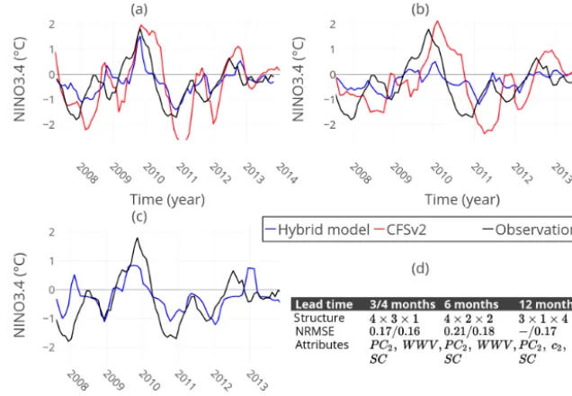
rela-Figure 7.NINO3.4 predictions of the CFSv2 ensemble mean (red) and the hybrid model with ARIMA(12,1,0) (blue), compared to the observed index (black). For the hybrid model predictions, from an ensemble of 84 different ANN structures, structures resulting in a low NRMSE are presented.(a)The 3-month lead time prediction of CFSv2 and 4-month lead time prediction of the hybrid model,(b)the 6-month lead time predictions and(c)12-month lead prediction. The CFSv2 ensemble does not predict 12 months ahead.(d)Table containing information about all predictions: ANN structures of the hybrid model, NRMSEs of the CFSv2 ensemble mean and the hybrid model, and attributes used in the hybrid model predictions.
tively simple ANN structure within an ensemble consisting of 84 different ANN structures are also shown in Fig. 7. The 84 different structures are all structures up to three hidden layers with up to four neurons.
Comparing the 3-month lead prediction of the CFSv2 en-semble with the 4-month lead prediction of the hybrid model, both the amplification and the lag of the hybrid model pre-diction are smaller. While the lead time of the hybrid model is 1 month longer, the prediction skill is better in terms of NRMSE. The prediction skill of the hybrid model decreases at a 6-month lead compared to the 4-month lead time diction. Thereby the lag and amplification of the CFSv2 pre-diction increase. Although the hybrid model does not suffer as much from the lag, it underestimates the El Niño event of 2010. In terms of NRMSE the hybrid model still obtains a better prediction skill.
Although the shorter lead time predictions show slightly better results than the conventional models, most important is a good prediction skill for larger lead times that appears to overcome the spring predictability barrier. To perform a 12-month lead prediction which could overcome this barrier, the attributes from the shorter lead time predictions are found to be insufficient. However,c2of the SSH network has shown to be predictive at this lead time, according to its Granger causality and cross-correlation. Therefore the WWV is re-placed byc2for this prediction, which is related to the same physical mechanism. In terms of NRMSE, the 12-month lead
prediction even improves the 6-month lead prediction of the hybrid model. On average the prediction does not contain a lag in this period.
The hyperparameter values (i.e. the ARIMA order and the ANN structure) of the predictions in Fig. 7 could still be a lucky shot. Therefore the spread of the predictions with dif-ferent hyperparameter values is shown in Fig. 8. For the ANN structures, nine optimal (in terms of NRMSE) predictions from the ensemble of 84 are considered. This resulted in a higher spread in the 6- and 12-month lead prediction com-pared to the 4-month lead prediction. For the ARIMA order all 9≤p≤14 are chosen, which resulted in almost no spread for the 3- and 12-month lead prediction and a higher spread in the 6-month lead prediction. Overall the models converge to similar predictions for those different hyperparameter val-ues.
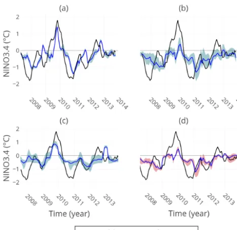
Figure 8. Spread and mean (blue line) of ensembles of hybrid model predictions with different hyperparameter values. The nine optimal (in terms of NRMSE) predictions from the 84 different ANN structures at the (a) 4-month lead time, (b) 6-month lead time and(c)12-month lead time. (d)Ensemble with 9≤p≤14 in the ARIMA order with their optimal ANN structure at 6-month lead time prediction (at the 4- and 12-month lead there is almost no spread). Black is the observed NINO3.4 index.
Figure 9.Cross-validation results of the(a)4-,(b)6- and(c) 12-month lead predictions of hybrid models from Fig. 7. Each line presents the frequency every NRMSE is obtained for 200 different initial test sets with a specific training set/test set percentage split. The vertical dashed line denotes the NRMSE of the predictions of Fig. 7.
Figure 10.NINO3.4 prediction from May 2017. In black the ob-served index until May 2017. Red is the CFSv2 ensemble predic-tion mean and the shaded area is the spread of the ensemble. The hybrid model prediction in blue is given by predictions from hybrid models found to be most optimal at the different lead times with ARIMA(12,1,0). The dashed blue line is the running 12-month lead time prediction.
The different percentage splits are chosen since the size of a training set could possibly have an influence on the predic-tion model. The cross-validapredic-tion results of the hybrid mod-els of Fig. 7 are presented in Fig. 9. At all three prediction lead times, the peaks coincide at the same NRMSE for dif-ferent training–test set ratios. Therefore the difdif-ferent sizes of training and test sets do not seem to influence the result. However, the width of the peaks increases when the predic-tion lead time increases. This implies the predicpredic-tion skill be-comes more sensitive to the choice of the training and test set with higher lead time. Interestingly, at the 4- and 6-month lead time predictions, the average NRMSE is lower than the NRMSE of the prediction of Fig. 7. This implies the predic-tions with a different training and test set are on average even better than the prediction shown in Fig. 7.
Finally, a prediction is made for the coming year in Fig. 10. Different hybrid models are used at different lead times with ARIMA(12,1,0). ANN structures are chosen that are found to be optimal at the different lead times. For the predictions up to 5 months, the attributes WWV, PC2 and the SC are used from 1980 until the present. For the 12-month lead predic-tion, the WWV is replaced byc2again. This timec2is com-puted from the SSALTO/DUACS dataset. Therefore, only a dataset from 1993 until the present has been used to train the model and perform the 12-month lead prediction.
coming 9 months. The hybrid models predict development to a strong La Niña (NINO3.4 index lower than −1.5) the coming year. From the time of writing, only time will tell which prediction is better. By the time of submission in early March 2018, La Niña conditions are present according to the Climate Prediction Centre of NCEP.
5 Summary and discussion
A successful attempt was made in this paper to use ma-chine learning (ML) techniques in a hybrid model to im-prove the skill of El Niño predictions. Crucial for the success of this hybrid model is the choice of the attributes applied to the artificial neural network. Here, we have explored the use of network variables as additional attributes to several physical ones. Results of the ZC model provided several in-teresting network variables. Of these network variables, c2 the amount of clusters of size two in a sea surface height (SSH) network constructed from observations, is found to provide a warning of a percolation-like transition in the SSH network. This percolation-like transition coincides with an El Niño event. This variable relates to the WWV and hence the recharge/discharge mechanism, but extends the predic-tion lead time of the WWV when applied in the predicpredic-tion scheme. Furthermore, apart from both these quantities re-lated to “recharge/discharge”, the PC2and the seasonal cycle (SC) improve the prediction skill, representing respectively the WWBs and the phase locking of ENSO. The flexibility of implementing different variables at different lead times al-lows the hybrid model to improve on the CFSv2 ensemble at short lead times (up to 6 months). Furthermore, it had a better prediction result than all members of the CFSv2 ensemble in January 2010.
By including the network variablec2, we obtained a 12-month lead time prediction with comparable skill to the pre-dictions at shorter lead times. This prediction shows a step towards beating the spring predictability barrier. Using ML has the advantage of recognizing the early warning signal of c2 as either a false or true positive. Therefore, it can be a more reliable method then considering a warning when the signal exceeds a certain threshold (Ludescher et al., 2014). Moreover, the early signal from the network variable is not only used to predict an El Niño event, but the development of ENSO, as the hybrid model provides a regression of the NINO3.4 index. ML serves as a tool which is able to rec-ognize important, but subtle, patterns. Something the con-ventional statistical and dynamical models fail to do in the chaotic system. In the end, the predictions from May 2017 are discussed. By the time of writing, this is the prediction for the coming year. The CFSv2 ensemble mean predicts neutral conditions for the coming 9 months, with the spread between different members ranging from a strong El Niño to a mod-erate La Niña. The hybrid model predicts modmod-erate to strong La Niña conditions for the coming year.
Although the results of the methods are promising, some adaptations to the methods which select attributes could still improve predictions. Several network variables resulted in a clear signal in the ZC model, but not necessarily for the observations. Perhaps the cross-correlation and a Granger causality test are not enough to determine the suitability of a variable in the observations. Testing all possible attribute sets in the prediction scheme and comparing results costs time. As a solution, the nonlinear methods “lagged mutual information” and “transfer entropy” can be techniques to se-lect variables at different lead times. After all, the attributes are applied in the nonlinear part of the prediction scheme. Consequently, more variables might be found to increase the prediction skill.
Even though the currently applied network measures showed interesting properties, different climate network con-struction methods can still be interesting to apply. The Pear-son correlation is a simple, effective method to define links between nodes. However, different properties of climate net-works could be found when using mutual information in-stead. Moreover, the effect of spatial distance between nodes can be investigated and corrected for Berezin et al. (2012). Besides, we have limited ourselves to networks within the Pacific area itself. As ENSO is an important mode in the whole climate system, the area used for network construc-tion might as well be extended. More specifically, it can be interesting to include the Indian Ocean in the network con-struction. Evidence is found that a cold SST to the west of the Indian Ocean is related to a WWB a few months later (Wieners et al., 2016). This could result in a variable related to WWBs, but increasing the lead compared to PC2, which is comparable toc2increasing the lead compared of the WWV. By applying the ARIMA as a simple yet effective statisti-cal method to apply in the first step of the scheme, the hybrid model shows promising results. However, the exact reason for how this model works remains a topic of investigation. The ARIMA prediction could be related to the linear wave dynamics. It can be interesting to replace the ARIMA part of the scheme by a dynamical model accounting for these linear wave dynamics. For the same reason, vector autoregression can be used instead of ARIMA. Being a multivariate gener-alization of an autoregressive model, this can implement the linear effect of other variables on ENSO.
dynam-ics by themselves, by combining them with a purely linear model. Moreover, the applied methods searched for a predic-tion model which is most optimal in terms of least squares minimization. However, it could be interesting to put larger weight on predicting the extreme events in the optimization scheme (as the 6-month lead predictions missed the 2010 El Niño event in Fig. 8), or find a function which is simpler (e.g. applying a support vector machine instead of ANN; Pai and Lin, 2005).
A general difficulty in El Niño prediction is the short avail-able observational time series, also in other statistical predic-tion models (Drosdowsky, 2006). Although different hyper-parameters (the ANN structure and ARIMA order) converge to a similar prediction and the prediction models perform well at different training and test sets, the short time series makes it difficult to perform another cross-validation method which completely rules out that the model is overfitting.
Appendix A
This appendix summarizes the methods to calculate climate network properties. The methods improved the prediction in the ZC model, but not for observational data. Thus, they are not discussed in the main text. Appendix A1 defines the dif-ferent quantities and Appendix A2 their application to the ZC model.
A1 Alternative network methods
From the unweighted network we compute the local degree di of nodeiin the network as
di=
X
j
Aij, (A1)
i.e. degreedi is equal to the amount of nodes that are con-nected to nodei.
The spatial symmetry of the degree distribution is of in-terest, since it informs where most links of the network are located. More specifically, our interest will be in the symme-try in the zonal direction in a network. Therefore, the skew-ness of the meridional mean of the degree in the network is calculated. This defines the zonal skewness of the degree dis-tribution in a network.
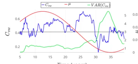
The following two climate network properties are derived from a so-called NetOfNet approach. This is a network con-structed with the same methods as previously, but using multiple variables at each grid point (as specified in Ap-pendix A2). This gives a network consisting of the networks from the different variables interacting with each other. Only NetOfNet of two different variables are considered. First, the cross clustering contains information about the interaction between two unweighted networks. The local cross cluster-ing of a node is the probability that two connected nodes in the other network are also connected to each other. The global cross clustering Cvw is the average over all nodes in subnetworkGvof the cross clustering betweenGvandGw:
Cvw= 1 Nv
X
r 1 kr(kr−1)
X
p6=q
ArpApqAqr. (A2)
Hereris a node in subnetworkGvof sizeNv,pandqare the nodes in the other subnetworkGw, andkr denotes the cross degree of noder(i.e. amount of cross links noderhas with the other subnetwork).
The second NetOfNet property is the algebraic connectiv-ity. This is the second smallest eigenvalue (λ2) of the Lapla-cian matrix as in Newman (2010) and describes the “diffu-sion” of information in the network. In general,λ2>0 if the network has a single component.
A final network property 1 makes use of a differently calculated network which is also undirected, but weighted. To construct it, the cross-correlation Cij(1t) at lag 1t, i.e. the Pearson correlation between the variables pi(t) and
Figure A1.Global cross clustering between the SST and wind-stress network in blue and its variance in green in the ZC model. The coupling strengthµdefined as a sinusoid aroundµc=3 with an amplitude of 0.25 is in red. The sliding window is applied with a window of 5 years.
pj(t+1t) is considered. Then the weights between the nodes are calculated by
Wij=
max1t(Cij)−mean(Cij) SD(Cij)
. (A3)
Here max1t denotes the maximum, SD the standard devia-tion and mean the mean value over all time steps that are considered.
To calculate the property1of the network, links are added to a network one by one, adding the link with the largest weight first (Eq. A3). At every stepT that a link is added, the size of the largest clusterS1(T) is calculated. At the point of the percolation transition,S1(T) increases rapidly. The size of this jump is1:
1=max [S1(2)−S1(1),···, S1(T+1)−S1(T),···]. (A4)
The quantity1can be used to capture the percolation-like transition (Meng et al., 2017).
A2 Climate network properties of the ZC model
Determining how strong noise can excite the ENSO mech-anisms in the subcritical case, or determining whether the feedbacks sustain an oscillation in the supercritical state, could provide information to increase the prediction skill. Feng (2015) found that the skewness of the degree dis-tribution Sd of the network reconstructed from SST de-creases monotonically with increasing coupling strengthµ. Although Sd relates to the climate stability and coupling strength, it does not inform whether the system is in either the supercritical or subcritical state.
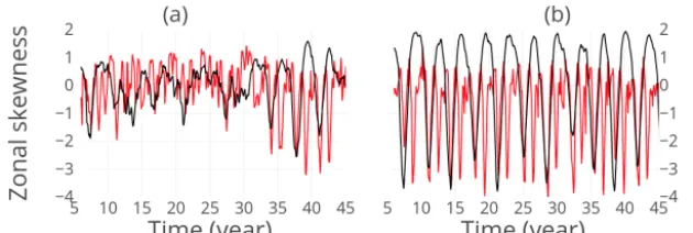
Figure A2.Zonal skewness of the degree field of the thermocline network with=0.6 and a sliding window of 1 year in red, NINO3.4 index in black in the ZC model.(a)The subcritical (µ=2.7) and(b)the supercritical (µ=3.25) case.
nodes. In Fig. A1, this cross clustering is calculated from data from the ZC model, when coupling strength µchanges pe-riodically in time around the critical value µc∼3.0. Under subcritical conditions, the noise has a larger influence on lo-cal correlations. This causes triangles to break and the vari-ance in the cross clustering coefficient to increase. The cross clusteringCvwis hence a diagnostic network variable which informs whether the state of the system is in the supercritical or subcritical regime.
Second, from the classical view of the oscillatory be-haviour of ENSO, waves in the thermocline should contain memory of the system, because of their negative delayed feedback. The changing structure of the thermocline network is therefore of interest when predicting ENSO. Calculating this network with threshold =0.6 and a sliding window with a length of 1 year, a zonal pattern in the change of the network close to the equator can be observed during an ENSO cycle. To compare network structures in the super-and subcritical state, now constantµ=2.7 (subcritical) and µ=3.25 (supercritical) are taken. Generally, the degree field is quite spatially symmetric, but when the ENSO turns either from upward to downward, or from downward to upward, the degree of the nodes in the east decreases. This is at the peak El Niño or La Niña.
To capture this zonal asymmetry around the equator with a variable, the zonal skewness of the degree field will be used between 7◦S to 7◦N. The higher the skewness, the more the degree will be located west of the basin. If the skewness is close to zero, the degree is symmetrically distributed over the basin. If it is low, most of the degree is situated in the east. The skewness will show a negative peak when the ENSO in-dex is at its highest or lowest point in the cycle (Fig. A2). In the supercritical caseµ=3.25 this effect is indeed observed. Nevertheless, in the subcritical case, the pattern is only vis-ible once the ENSO index shows a clear oscillation (around year 32).
Third, the quantity1behaves similar to c2, when calcu-lated from the same (thermocline) network. Although1does not depend on a chosen threshold likec2, it peaks closer to an El Niño event.
Data availability. All used observational data are from third par-ties and are either cited or can be found by URL as specified in Sect. 2.1.
Competing interests. The authors declare that they have no con-flict of interest.
Acknowledgements. Peter D. Nooteboom would like to thank the Instituto de Física Interdisciplinar y Sistemas Complejos (IFISC), for hosting his stay in Mallorca during part of 2017.
Cristóbal López and Emilio Hernández-García acknowledge support from Ministerio de Economia y Competitividad and Fondo Europeo de Desarrollo Regional through the LAOP project (CTM2015-66407-P, MINECO/FEDER)
Edited by: Ben Kravitz
Reviewed by: Robert Link and one anonymous referee
References
Akaike, H.: A New Look at the Statistical Model Iden-tification, IEEE T. Automat. Contr., AC-19, 716–723, https://doi.org/10.1109/TAC.1974.1100705, 1974.
Aladag, C. H., Egrioglu, E., and Kadilar, C.: Forecasting nonlinear time series with a hybrid methodology, Appl. Math. Lett., 22, 1467–1470, https://doi.org/10.1016/j.aml.2009.02.006, 2009. Al-Smadi, A. and Al-Zaben, A.: ARMA Model Order
Determina-tion Using Edge DetecDetermina-tion: A New Perspective, Circuits, Sys-tems Signal Processing, 24, 723–732, 2005.
Berezin, Y., Gozolchiani, A., Guez, O., and Havlin, S.: Stabil-ity of Climate Networks with Time, Sci. Rep.-UK, 2, 1–8, https://doi.org/10.1038/srep00666, 2012.
Bergmeir, C. and Benítez, J. M.: On the use of cross-validation for time series predictor evaluation, Inf. Sci. (Ny)., 191, 192–213, https://doi.org/10.1016/j.ins.2011.12.028, 2012.
Bishop, C. M.: Pattern Recognition and Machine Learning, Springer-Verlag New York, 2006.
Bjerknes, J.: Atmospheric Teleconnections From The Equatorial Pacific, Mon. Weather Rev., 97, 163–172, https://doi.org/10.1175/1520-0493(1969)097<0163:ATFTEP>2.3.CO;2, 1969.
Bosc, C. and Delcroix, T.: Observed equatorial Rossby waves and ENSO-related warm water volume changes in the equatorial Pacific Ocean, J. Geophys. Res., 113, 1–14, https://doi.org/10.1029/2007JC004613, 2008.
Bunge, L. and Clarke, A. J.: On the Warm Water Volume and Its Changing Relationship with ENSO, J. Phys. Oceanogr., 44, 1372–1385, https://doi.org/10.1175/JPO-D-13-062.1, 2014. Chen, D., Cane, M. A., Kaplan, A., Zebiak, S. E., and Huang, D.:
Predictability of El Niño over the past 148 years, Nature, 428, 733–736, https://doi.org/10.1038/nature02439, 2004.
Deza, J. I., Masoller, C., and Barreiro, M.: Distinguishing the effects of internal and forced atmospheric variability in cli-mate networks, Nonlin. Processes Geophys., 21, 617–631, https://doi.org/10.5194/npg-21-617-2014, 2014.
Dijkstra, H. A.: The ENSO phenomenon: theory and mechanisms, Adv. Geosci., 6, 3–15, https://doi.org/10.5194/adgeo-6-3-2006, 2006.
Drosdowsky, W.: Statistical prediction of ENSO (Nino 3) using sub-surface temperature data, Geophys. Res. Lett., 33, 10–13, https://doi.org/10.1029/2005GL024866, 2006.
Fedorov, A. V., Harper, S. L., Philander, S. G., Winter, B., and Wit-tenberg, A.: How predictable is El Niño?, B. Am. Meteorol. Soc., 84, 911–919, https://doi.org/10.1175/BAMS-84-7-911, 2003. Feng, Q. Y.: A complex network approach to understand climate
variability, Ph.D. thesis, Utrecht University, 2015.
Feng, Q. Y. and Dijkstra, H. A.: Climate Network Stabil-ity Measures of El Niño VariabilStabil-ity, Chaos, 27, 035801, https://doi.org/10.1063/1.4971784, 2016.
Feng, Q. Y., Vasile, R., Segond, M., Gozolchiani, A., Wang, Y., Abel, M., Havlin, S., Bunde, A., and Dijkstra, H. A.: Cli-mateLearn: A machine-learning approach for climate predic-tion using network measures, Geosci. Model Dev. Discuss., https://doi.org/10.5194/gmd-2015-273, 2016.
Fountalis, I., Bracco, A., and Dovrolis, C.: ENSO in CMIP5 simulations: network connectivity from the recent past to the twenty-third century, Clim. Dynam., 45, 511–538, https://doi.org/10.1007/s00382-014-2412-1, 2015.
Gill, A.: Some simple solutions for heat-induced tropical circula-tion, Q. J. Roy Meteor. Soc., 106, 447–462, 1980.
Goddard, L., Mason, S., Zebiak, S., Ropelewski, C., Basher, R., and Cane, M.: Current Approaches to seasonal-to-interannual climate predictions, Int. J. Climatol., 21, 1111–1152, https://doi.org/10.1080/002017401300076036, 2001.
Gozolchiani, A., Yamasaki, K., Gazit, O., and Havlin, S.: Pattern of climate network blinking links follows El Niño events, EPL (Europhysics Letters), 83, 28005, https://doi.org/10.1209/0295-5075/83/28005, 2008.
Gozolchiani, A., Havlin, S., and Yamasaki, K.: Emer-gence of El Niño as an autonomous component in the climate network, Phys. Rev. Lett., 107, 1–5, https://doi.org/10.1103/PhysRevLett.107.148501, 2011. Guyon, I. and Elisseeff, A.: An Introduction to Variable and
Feature Selection, J. Mach. Learn. Res., 3, 1157–1182, https://doi.org/10.1016/j.aca.2011.07.027, 2003.
Hall, M. A.: Correlation-based Feature Selection for Machine Learning, Ph.D. thesis, The university of Waikato, 1999. Hibon, M. and Evgeniou, T.: To combine or not to combine:
Se-lecting among forecasts and their combinations, Int. J. Forecast-ing, 21, 15–24, https://doi.org/10.1016/j.ijforecast.2004.05.002, 2005.
Huang, B., Banzon, V. F., Freeman, E., Lawrimore, J., Liu, W., Peterson, T. C., Smith, T. M., Thorne, P. W., Woodruff, S. D., and Zhang, H. M.: Extended reconstructed sea surface temper-ature version 4 (ERSST.v4). Part I: Upgrades and intercompar-isons, J. Climate, 28, 911–930, https://doi.org/10.1175/JCLI-D-14-00006.1, 2015.
Hush, M. R.: Machine learning for quantum physics, Science, 355, 580, https://doi.org/10.1126/science.aam6564, 2017.
Jin, F.-F., Neelin, D. J., and Ghil, M.: El Niño on the Devil’s stair-case: Annual Subharmonic Steps to Chaos, Science, 264, 70–72, https://doi.org/10.1126/science.264.5155.70, 1994.
Khashei, M. and Bijari, M.: A novel hybridization of artifi-cial neural networks and ARIMA models for time series forecasting, Applied Soft Computing Journal, 11, 2664–2675, https://doi.org/10.1016/j.asoc.2010.10.015, 2011.
Latif, M., Biercamp, J., and von Storch, H.: The response of a Coupled Ocean-Atmosphere General Circulation Model to Wind Bursts, J. Atmos. Sci., 45, 964–979, 1988.
Ludescher, J., Gozolchiani, A., Bogachev, M. I., Bunde, A., Havlin, S., and Schellnhuber, H. J.: Very early warning of next El Niño., P. Natl. Acad. Sci. USA, 111, 2064–2066, https://doi.org/10.1073/pnas.1323058111, 2014.
Madden, R. A. and Julian, P. R.: Observations of the 40–50-Day Tropical Oscillation—A Review, Mon. Weather Rev., 122, 814–837, https://doi.org/10.1175/1520-0493(1994)122<0814:OOTDTO>2.0.CO;2, 1994.
Meng, J., Fan, J., Ashkenazy, Y., and Havlin, S.: Percolation framework to describe El Niño conditions, Chaos, 27, 1–15, https://doi.org/10.1063/1.4975766, 2017.
Moore, A. M. and Kleeman, R.: Stochastic forcing of ENSO by the intraseasonal oscillation, J. Cli-mate, 12, 1199–1220, https://doi.org/10.1175/1520-0442(1999)012<1199:SFOEBT>2.0.CO;2, 1999.
National Oceanic and Atmospheric Administration: Upper Ocean Heat Content and ENSO, https://www.pmel.noaa.gov/elnino/ upper-ocean-heat-content-and-enso, last access: May 2017. Newman, M.: Networks: An introduction, vol. 6, Oxford
univer-sity press, Oxford, https://doi.org/10.1017/S1062798700004543, 2010.
Pai, P.-F. and Lin, C.-S.: A hybrid ARIMA and support vector ma-chines model in stock price forecasting, Omega, 33, 497–505, https://doi.org/10.1016/j.omega.2004.07.024, 2005.
Philander, S. G.: El Nino, La Nina, and the Southern Oscillation, vol. 46, International Geophysics Series, San Diego, 1990. Rayner, N. A., Parker, D. E., Horton, E. B., Folland, C. K.,
Alexan-der, L. V., Rowell, D. P., Kent, E. C., and Kaplan, A.: Global analyses of sea surface temperature, sea ice, and night marine air temperature since the late nineteenth century, J. Geophys. Res., 108, D14, https://doi.org/10.1029/2002JD002670, 2003. Rebert, J. P., Donguy, J. R., Eldin, G., and Wyrtki, K.: Relations
between sea level, thermocline depth, heat content, and dynamic height in the tropical Pacific Ocean, J. Geophys. Res., 90, 11719, https://doi.org/10.1029/JC090iC06p11719, 1985.
Rissanen, J.: Modelling by the shortest data description, Automat-ica, 14, 465–471, 1978.
Rodríguez-Méndez, V., Eguíluz , V. M., Hernández-García, E., and Ramasco, J. J.: Percolation-based precursors of transitions in extended systems, Sci. Rep.-UK, 6, 29552, https://doi.org/10.1038/srep29552, 2016.
Runge, J. G.: Detecting and Quantifying Causal Interactions from Time Series of Complex Systems, Ph.D. thesis, Humboldt-Universität zu Berlin, 2014.
Steinhaeuser, K., Ganguly, A. R., and Chawla, N. V.: Multivari-ate and multiscale dependence in the global climMultivari-ate system re-vealed through complex networks, Clim. Dynam., 39, 889–895, https://doi.org/10.1007/s00382-011-1135-9, 2012.
Stolbova, V., Martin, P., Bookhagen, B., Marwan, N., and Kurths, J.: Topology and seasonal evolution of the network of extreme precipitation over the Indian subcontinent and Sri Lanka, Nonlin. Processes Geophys., 21, 901–917, https://doi.org/10.5194/npg-21-901-2014, 2014.
Sun, Y., Li, J., Liu, J., Chow, C., Sun, B., and Wang, R.: Using causal discovery for feature selection in multi-variate numerical time series, Mach. Learn., 101, 377–395, https://doi.org/10.1007/s10994-014-5460-1, 2014.
Tsonis, A. A., Swanson, K. L., and Roebber, P. J.: What do networks have to do with climate?, B. Am. Meteorol. Soc., 87, 585–595, https://doi.org/10.1175/BAMS-87-5-585, 2006.
Tziperman, E., Stone, L., Cane, M. A., and Jarosh, H.: El Nino chaos: Overlapping of resonances between the seasonal cycle and the pacific ocean-atmosphere oscillator, Science, 264, 72– 74, https://doi.org/10.1126/science.264.5155.72, 1994.
Valenzuela, O., Rojas, I., Rojas, F., Pomares, H., Herrera, L. J., Guillen, A., Marquez, L., and Pasadas, M.: Hy-bridization of intelligent techniques and ARIMA models for time series prediction, Fuzzy Set. Syst., 159, 821–845, https://doi.org/10.1016/j.fss.2007.11.003, 2008.
van der Vaart, P. C. F., Dijkstra, H. A., and Jin, F. F.: The Pacific Cold Tongue and the ENSO Mode: A Uni-fied Theory within the Zebiak–Cane Model, J. At-mos. Sci., 57, 967–988, https://doi.org/10.1175/1520-0469(2000)057<0967:TPCTAT>2.0.CO;2, 2000.
von der Heydt, A. S., Nnafie, A., and Dijkstra, H. A.: Cold tongue/Warm pool and ENSO dynamics in the Pliocene, Clim. Past, 7, 903–915, https://doi.org/10.5194/cp-7-903-2011, 2011. Wang, Y., Gozolchiani, A., Ashkenazy, Y., and Havlin, S.: Oceanic
El-Niño wave dynamics and climate networks, New J. Phys., 18, 1–5, https://doi.org/10.1088/1367-2630/18/3/033021, 2015. Wieners, C. E., de Ruijter, W. P., Ridderinkhof, W., von der
Heydt, A. S., and Dijkstra, H. A.: Coherent tropical Indo-Pacific interannual climate variability, J. Climate, 29, 4269– 4291, https://doi.org/10.1175/JCLI-D-15-0262.1, 2016. Wu, A., Hsieh, W. W., and Tang, B.: Neural network forecasts of the
tropical Pacific sea surface temperatures, Neural Networks, 19, 145–154, https://doi.org/10.1016/j.neunet.2006.01.004, 2006. Yeh, S.-W., Kug, J.-S., Dewitte, B., Kwon, M.-H., Kirtman, B. P.,
and Jin, F.-F.: El Niño in a changing climate, Nature, 461, 511– 514, https://doi.org/10.1038/nature08316, 2009.
Zebiak, S. E. and Cane, M. A.: A model El Niño-Southern Oscillation, Mon. Weather Rev., 115, 2262–2278, https://doi.org/10.1175/1520-0493(1987)115<2262:AMENO>2.0.CO;2, 1987.