Removal Efficiency in Industrial Scale Liquid Jet Ejector for Chlorine - Aqueous Caustic Soda System

(1)

ISSN: 2231-5381

http://www.ijettjournal.org

Page 2931

Removal Efficiency in Industrial Scale Liquid Jet

Ejector for Chlorine-Aqueous Caustic Soda System

K. S. Agrawal

Assistant Professor, Department of Chemical Engineering Faculty of Technology and Engineering, The M. S. University of Baroda,

Vadodara, Gujarat, India

Abstract— The prediction of removal efficiency of gas in liquid jet ejector is an important factor as it influences the design of the mass transfer equipment. The major factors which affect the efficiency of jet ejector are flow rates like gas and liquid and the concentration of absorbing liquid and solute in the gas. This paper deals with statistical modeling for removal efficiency of gas in multi nozzle jet ejector for industry scale jet ejector. The developed model is based on statistical techniques to predict removal efficiency for variation in gas and liquid Concentration. The model is simulated using STATGRAPHICS PLUS 4.0 software for plotting the response surface. The same model is validated by experimental data of industry scale jet ejector.

I. INTRODUCTION

Venturi scrubbers in general have been successfully employed for gas cleaning applications over the last five decades, as they show potential for meeting stringent emission standards. They are very efficient even for fine particulate removal. The removal efficiency is not only depending on scrubber geometry but also on the flow rates. There are some models which are available for the same and they are based on statistical techniques. The collection efficiency model used in

the algorithm is described in detail elsewhere

(Ananthanarayanan and Viswanathan, 1998 and 1999; Agrawal, 2012 and2013).

The present study focuses on multi nozzle liquid jet ejector which is one type of venturi scrubber. Liquid jet ejectors are those which are using a mechanical pump to generate a high velocity fluid jet. This fluid jet creates suction and another fluid is entrained into it by transfer of momentum.

Over and above compact construction the liquid jet ejectors can generate high interfacial area and can handle very hot, wet, inflammable and corrosive gases.

The major factors which affect the efficiency of liquid jet ejector are liquid flow rate, gas flow rate, the concentration of absorbing liquid and the concentration of the solute in the gas. Ravindram and Pyla (1986) proposed a theoretical model for

the absorption of and in dilute based on

simultaneous diffusion and irreversible chemical reaction for predicting the amount of gaseous pollutant removed. Agrawal (2012, 2013) proposed a statistical model for absorption of chlorine into aqueous NaOH solution.

Many researchers (Volgin et al., 1968; Ravindram and Pyla, 1986; Cramers et al., 1992, 2001; Gamisans et al., 2004,

2002; Mandal, 2003a, 2003b, 2004, 2005, 2005a, 2005b; Balamurugan et al., 2007, 2008; Utomo et al., 2008; Yadav, 2008; Li and Li, 2011.) have reported different theories and correlations to predict scrubbing efficiency of jet ejectors.

Uchida and Wen (1973) developed a mathematical model to predict the removal efficiency of 2 into water and alkali

solution. The simulated results of their model were compared with experimental results and they found that there is a good agreement with the experimental results. They have also found enhancement factor to predict rate of the chemical absorption.

Gamisans et al. (2002) evaluated the suitability of an ejector-venturi scrubber for the removal of two common stack gases, sulphur dioxide and ammonia. They studied the influence of several operating variables for different geometries of venturi tube. A statistical approach was presented by them to characterize the performance of scrubber by varying several factors such as gas pollutant concentration, gas flow rate and liquid flow rate. They carried out the computation by multiple regression analysis making use of the method of the least squares method. They have used

commercial software package, STATGRAPHICS, to

determine the multiple regression coefficients.

Less attention has been paid in the area of mathematical and statistical modeling. The statistical models have edge over other models due to their capacity to handle random data correctly. There are several techniques available to relate the controllable factors and experimental facts. Due to complex nature of affluent gases in terms of its concentration of constituents, temperature, quality and quantity, it requires experimentation to improve existing processes and to develop new ones.

This paper deals with factors affecting the efficiency of jet ejector to remove solute gases from the gas stream. The major factors which affect the efficiency of jet ejector are liquid flow rate, gas flow rate, the concentration of absorbing liquid and the concentration of the solute in the gas.

In this paper, we have made an attempt to develop statistical model based on non linear quadratic multiple regression analysis to predict removal efficiency of jet ejector

(2)

ISSN: 2231-5381

http://www.ijettjournal.org

Page 2932 II. MATHEMATICAL MODELLING

We have used the non linear quadratic relation between independent variables and dependent variables and is as follows:

=

Ψ

+

Ψ

X +

Ψ

X X … … … … . (1)

Here, is a response variable, is the main factor;Ψ is the constant value of the regression; Ψ is the linear coefficient; Ψ is the quadratic coefficient and Ψ is the interaction coefficient. When = ; Ψ =Ψ and 2Ψ = .The computation was carried out by non linear regression analysis making use of the generalized minimal residual method.

III. EXPERIMENTAL RESULTS

The experimental work was carried in industrial scale multi nozzle jet ejector and is as follows

A. Experimental set up

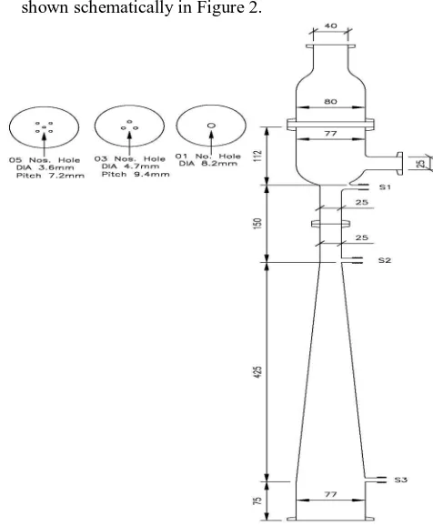
1. The experimental Setup for industry scale jet ejector is shown schematically in Figure 2.

Fig. 1 Detail of the jet ejector used in experimental setup

These experiments were conducted on industrial stage ejector. The details of ejector are shown in Figure 1 and Table 1.

2. The schematic flow diagram as in Figure 2 is self indicative.

3. The ejector is having 3 sample point S1, S2 and S3. Sample S0 is drawn from tank T1 directly. The air flow

rate is measured by using electronic anemometer. There is a rotameter for measuring flow rate and a soap film meter to calibrate the rotameter. There are two tanks T1 and T2. Tank T1 is used to prepare sodium hydroxide solution and tank T2 is ejector outlet tank. V1, V2, V3 and V4 are control valves. The pump P1 is provided to circulate sodium hydroxide solution through the ejector. Pressure gauge P1 is provided to measure the primary fluid pressure (water).

B. Experimental procedure

1. Before starting the experiment the rotameter for chlorine was calibrated by soap film meter.

2. The required nozzle plate was fitted.

3. The required sodium hydroxide concentration was

prepared by circulating the solution and operating valve V5, V4, V2 and V3.

Fig. 2 Schamatic diagram of experimental setup

4. The primary fluid (aqueous solutions) flow rate was adjusted to the required value by operating valve V5 and V4. The secondary air flow rate was measured by electronic anemometer. The flow rate is kept constant throughout the experiment.

5. The required chlorine rate was adjusted by operating valve V1. After the system reaches steady state the liquid sample S0, S1, S2 and S3 were drawn and analyzed.

6. The experiment was repeated for different concentrations of sodium hydroxide and chlorine and nozzle plates. The procedure was repeated for different set of liquid concentration and gas concentration. The results are compiled. The factors which affect the absorption efficiency are gas concentration and the scrubbing liquid concentration. In this work the jet ejector is operated on critical value of liquid flow rate. For a given geometry, reduction in the liquid flow rate will lead to reduction of induced gas flow rate. Therefore, in the present work the liquid flow rate is kept constant. Effect of

and , on the removal efficiency(% ) of the ejector

(3)

ISSN: 2231-5381

http://www.ijettjournal.org

Page 2933

TABLEI

DIMENSIONS OF EJECTORS

The experimental values for the operating variables used in the present work are presented and the experimental data are tabulated in Table 2 and 3

TABLEIII

CODIFICATION OF THE OPERATING VARIABLES FOR THE STATISTICAL

ANALYSIS

Code Variable Values

Gas concentration (kmole/m3)

(0.6 4.3) × 10

Liquid concentration (kmole/m3₎

0−0.95

Removal efficiency (%)

0–100

TABLEIIIII

EXPERIMENTAL MATRIX FOR CHLORINE REMOVAL EFFICIENCY USING SETUP

Run No.

Nozzle No.

10 ,

( / )

10

( / )

(%)

301 N5 2.95538 0.79 21.07

302 1.966803 0.79 43.18

303 1.475102 0.79 69.09

304 0.983402 0.79 97.88

321 N5 2.984934 0.57 47.42

322 1.986471 0.57 57.01

323 1.489853 0.57 57.01

324 0.993236 0.57 62.71

325 N5 2.984934 0.11 36.04

326 1.986471 0.11 34.20

327 1.489853 0.11 34.20

328 0.993236 0.11 34.20

305 N6 2.95538 0.79 17.24

306 1.966803 0.79 28.79

307 1.475102 0.79 19.19

308 0.983402 0.79 28.79

317 N6 2.95538 0.57 45.98

318 1.966803 0.57 57.58

319 1.475102 0.57 69.09

320 0.983402 0.57 63.33

329 N6 2.984934 0.11 49.32

330 1.986471 0.11 42.75

331 1.489853 0.11 38.00

332 0.993236 0.11 51.31

309 N7 2.95538 0.79 22.99

310 1.966803 0.79 28.79

311 1.475102 0.79 26.87

312 0.983402 0.79 23.03

313 N7 2.95538 0.57 19.16

314 1.966803 0.57 20.15

315 1.475102 0.57 19.19

316 0.983402 0.57 23.03

333 N7 2.984934 0.11 45.53

334 1.986471 0.11 62.71

335 1.489853 0.11 57.01

336 0.993236 0.11 45.61

Nozzle diameter ( ) DN 8.2 4.7 3.7

Number of Nozzle (orifice) n 1 3 5

Nozzle No. N5 N6 N7

pitch * 2

Area ratio (appx) ** 9.3

Diameter of Throat/ mixing tube

( ) 25

Length of Throat/ mixing tube ***

( ) 150

Projection ratio # 4.5

Angle of convergent well rounded

Angle of divergence of conical

diffuser ## 7

Length of the conical diffuser

( ) 425

Diameter of the diffuser exit ( ) 77

Diameter of the suction chamber

( ) DS 77

Length of the suction chamber

( ) 122

Distance between nozzle &

commencement of throat ( ) 112

Diameter of secondary gas inlet

( ) , 25

(4)

ISSN: 2231-5381

http://www.ijettjournal.org

Page 2934

TABLEIV

PARAMETERS FOR MULTIPLE REGRESSION ANALYSIS

IV. RESULTS AND INTERPRETATION

Statistical analysis

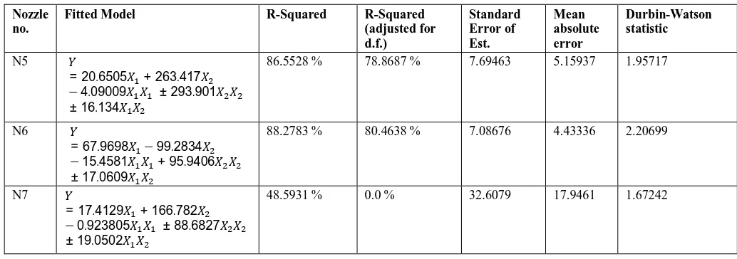
STATGRAPHICS Plus 4.0 is used to predict the removal efficiency (Y) using statistical model (equation 1) for the nozzles N5, N6 and N7.The results are summarized in Table 4 and 5. Table 4 demonstrates the parameters as outcome of simulated results of STATGRAPHICS plus 4.0. The regression coefficients of fitted models are summarized in table 5.

The analysis of variance (ANOVA) for the operational variables and , indicate that removal efficiency is well described by nonlinear quadratic models. The convergence is obtained successfully after 4 iterations for estimation of regression coefficients.

Furthermore, the statistical analysis showed that both

factors ( and , ) had significant effects on the

response ( ) and the liquid concentration is more

significant between two.

It may be observed that fitted models do not contain the independent term (Ψ ). This implies that the removal efficiency ( ) is a function of the factors considered only.

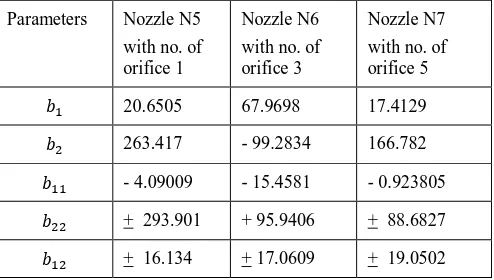
TABLEV

REGRESSION COEFFICIENT FROM MULTI REGRESSION ANALYSIS

Parameters Nozzle N5

with no. of orifice 1

Nozzle N6

Nozzle N7

20.6505 67.9698 17.4129

263.417 - 99.2834 166.782

- 4.09009 - 15.4581 - 0.923805

+ 293.901 + 95.9406 + 88.6827

+ 16.134 + 17.0609 + 19.0502

Tests are run to determine the goodness of fit of a model and how well the non linear regression plot approximates the experimental data. As the results are multi numerical they are presented in Figures 3 to 17 and Tables 6 to 17. Statistical tests like R-squared, R-squared (adjusted for d.f.), standard error of estimate, mean absolute error and Durbin-Watson statistic are covered. The tables containing confidence interval, analysis of variance (ANOVA) and residual analysis are also reported.

Properties to be Operated

Nozzle N5 with no. of orifice 1

Adopted Technique Nonlinear Regression Nonlinear Regression Nonlinear Regression

Dependent variable

Independent variables , , ,

Function to be estimated

+

+ +

+

+ +

+

+ +

Initial parameter estimates

=0.1 =0.1 =0.1 =0.1 =0.1

Estimation method Marquardt Marquardt Marquardt

Estimation stopped due to convergence of residual sum of squares.

Estimation stopped due to convergence of parameter estimates.

Number of iterations 4 4 4

Number of function calls

26 26 25

Fitted model

= 20.6505 + 263.417

−4.09009

± 293.901 ± 16.134

= 67.9698 −99.2834

−15.4581 + 95.9406

± 17.0609

= 17.4129 + 166.782

−0.923805

(5)

ISSN: 2231-5381

http://www.ijettjournal.org

Page 2935

A. Results of statistical analysis in STATGRAPHICS Plus 4 for different nozzles:

Nozzle N5 with no. of orifice 1

TABLEVI

ESTIMATION RESULTS FOR NOZZLE N5

Para-meter

Estimate Asymptotic

Standard Error

Asymptotic 95.0%Confidence Interval

Lower Upper

b1 20.6505 8.51199 0.522786 40.7782

b2 263.417 42.0993 163.868 362.966

b11 - 4.09009 2.9974 -11.1778 2.99764

b22 - 293.901 46.3188 -403.427 -184.374

b12 - 16.134 9.4982 -38.5937 6.32578

TABLEVII

ANALYSIS OF VARIANCE FOR NOZZLE N5

Source Sum of Squares Df Mean Square

Model 24459.2 5 4891.85

Residual 414.451 7 59.2073

Total 24873.7 12

Total (Corr.) 3082.07 11

TABLEVIII

RESULTS OF STATISTICAL TESTS FOR NOZZLE N5

R-Squared 86.5528 %

R-Squared (adjusted for d.f.) 78.8687 %

Standard Error of Est. 7.69463

Mean absolute error 5.15937

Durbin-Watson statistic 1.95717

TABLEIX

RESIDUAL ANALYSIS FOR NOZZLE N5

Estimation Validation

N 12

MSE 59.2073

MAE 5.15937

MAPE 14.7485

ME 0.271349

MPE -0.381023

Fig. 3 Removal efficiency (Y) versus gas concentration (X1) for constant

liquid concentration (X2 = 0.4) for nozzle N5

Fig. 4 Removal efficiency (Y) response surface versus gas concentration (X1)

and liquid concentration (X2) for nozzle N5

Fig. 5 Contour plot for removal efficiency (Y) for nozzle N5

Fig. 6 Predicted removal efficiency (Y) versus observed removal efficiency (Y) for nozzle N5

X2=0,4

Plot of Fitted Model

X1

Y

0,9 1,3 1,7 2,1 2,5 2,9 3,3 0

20 40 60 80

Estimated Response Surface

X1

X2

Y

0,9 1,3 1,7 2,1 2,5 2,9 _3,3 0 0,2 0,4 0,6

0,8 0

20 40 60 80

Contours of Estimated Response Surface

0,9 1,3 1,7 2,1 2,5 2,9 3,3

X1

0 0,2 0,4 0,6 0,8

X

2

Y 0,0 8,0 16,0 24,0 32,0 40,0 48,0 56,0 64,0 72,0

Plot of Y

0 20 40 60 80

predicted

0 20 40 60 80

ob

se

rv

e

(6)

ISSN: 2231-5381

http://www.ijettjournal.org

Page 2936

Fig. 7 Residual plot for nozzle N5

TABLEX

ESTIMATION RESULTS FOR NOZZLE N6

Parameter Estimate Asymptotic

Standard Error

Asymptotic 95.0% Confidence Interval

b1 67.9698 7.85634 48.746 87.1937

b2 -99.2834 42.5687 -203.445 4.87873

b11 -15.4581 2.76621 -22.2268 -8.6894

b22 95.9406 44.9216 -13.9789 205.86

b12 -17.0609 10.17 -41.9459 7.82414

TABLEXI

ANALYSIS OF VARIANCE FOR NOZZLE N6

Model 14787.6 5 2957.52

Residual 301.333 6 50.2222

Total 15088.9 11

Total (Corr.) 2570.73 10

TABLEXII

RESULTS OF STATISTICAL TESTS FOR NOZZLE N6

R-Squared 88.2783 %

TABLEXIII

RESIDUAL ANALYSIS FOR NOZZLE N6

N 11

MSE 50.2222

MAE 4.43336

MAPE 17.9304

ME 0.347291

MPE -0.243646

Fig. 8 Removal efficiency (Y) versus gas concentration (X1) for constant

Fig. 9 Removal efficiency (Y) response surface versus gas concentration (X1)

and liquid concentration (X2) for nozzle N6

Fig. 10 Contour plot for removal efficiency (Y) for nozzle N6

Residual Plot

0 20 40 60 80

predicted Y

-2 -1 0 1 2

S

tu

d

e

n

ti

z

e

d

r

e

si

d

u

a

l

X2=0,4

Plot of Fitted Model

0,9 1,3 1,7 2,1 2,5 2,9 3,3

X1

19 29 39 49 59 69

Y

Estimated Response Surface

0,9 1,3 1,7 2,1 2,5 2,9 3,3

X1

0 0,2 0,4 0,6

0,8

X2

-8 12 32 52 72 92

Y

Contours of Estimated Response Surface

0,9 1,3 1,7 2,1 2,5 2,9 3,3

X1 0

0,2 0,4 0,6 0,8

X

2

(7)

ISSN: 2231-5381

http://www.ijettjournal.org

Page 2937

Fig. 11 Predicted removal efficiency (Y) versus observed removal efficiency (Y) for nozzle N6

Fig. 12 Residual plot for nozzle N6

TABLE XIV Estimation Results for nozzle N7

Paramet er

Estimate Asymptotic

Standard Error

Confidence Interval Asymptotic 95.0%

b1 17.4129 17.0439 -20.5635 55.3892

b2 166.782 82.0164 -15.962 349.527

b11 -0.923805 3.77345 -9.33159 7.48398

b22 -88.6827 92.8142 -295.486 118.121

b12 -19.0502 14.3113 -50.9379 12.8375

TABLE XV

Analysis of Variance for nozzle N7

Model 64257.3 5 12851.5

Residual 10632.7 10 1063.27

Total 74890.1 15

Total (Corr.) 7155.6 14

TABLE XVI

Results of statistical tests for nozzle N7

R-Squared -48.5931 %

TABLE XVII Residual Analysis for nozzle N7

N 15

MSE 1063.27

MAE 17.9461

MAPE 43.8221

ME 4.7561

MPE -14.4586

Fig. 13 : Removal efficiency (Y) versus gas concentration (X1) for constant

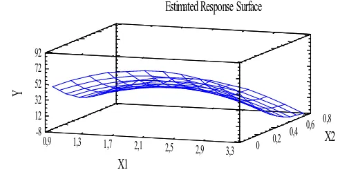
Fig. 14: Removal efficiency (Y) response surface versus gas concentration (X1) and liquid concentration (X2) for nozzle N7

Plot of Y

0 20 40 60 80

predicted

0 20 40 60 80

o

b

se

rv

e

d

Residual Plot

19 29 39 49 59 69

predicted Y

-3,2 -1,2 0,8 2,8 4,8

S

tu

d

e

n

ti

z

e

d

r

e

si

d

u

a

l

X2=0,5

Plot of Fitted Model

X1

Y

0 1 2 3 4 5

0 20 40 60 80 100

Estimated Response Surface

X1

X2

Y

0 ₁ ₂ ₃

4 ₅ 0 0,2 0,40,6

0,8 1 0

(8)

ISSN: 2231-5381

http://www.ijettjournal.org

Page 2938

Fig. 15: Contour plot for removal efficiency (Y) for nozzle N7

Fig. 16: Predicted removal efficiency (Y) versus observed removal efficiency (Y) for nozzle N7

Fig. 17: Residual plot for nozzle N7

B. Interpretation of the results of statistical analysis in STATGRAPHICS Plus 4 for different nozzles

The results of fitted model, R-squared test, R-squared (adjusted for d.f.) test, standard error of estimates, mean absolute error and Durbin-Watson statistic test are summarized in Table 18 and may be interpreted as follow.

 The R-Squared statistic indicates that the model as fitted explains 86.55 %, 88.27% and 48.59% of the variability in Y for N5, N6 and N7 respectively.

 The adjusted R-Squared statistic which is more suitable for comparing models with different numbers of independent variables are 78.86%, 80.46% and 0.0% for , N5, N6 and N7 respectively

 The standard error of the estimate shows the standard deviation of the residuals to be 7.69, 7.08 and 32.60 for N5, N6 and N7 respectively. This value can be used to construct prediction limits for new observations.

 The mean absolute error (MAE) of 5.15, 4.43 and 17.94 is

the average value of the residuals for N5, N6 and N7 respectively

 The Durbin-Watson (DW) statistic tests the residuals to determine if there is any significant correlation based on the order in which they occur. Similarly, since, the DW value is greater than 1.4 for N5, N6, N7 there is probably not any serious autocorrelation in the residuals.

 The output also shows asymptotic 95.0% confidence

intervals for each of the unknown parameters.

Interpretation of figures (graphs)

For each set of experiment a mathematical model describing the effect of related variables on removal efficiency were derived and plotted in the Figures 3 to 17.These figures may be analyzed as follows:

Figures 4, 9 and 14 show the response surfaces for the removal of chlorine with variation in initial gas concentration and the scrubbing liquid concentration. The response surface shows removal efficiency varies from 50% to maximum value of 95%. It is observed that the effect of liquid concentration is greater than the gas concentration on .

Dependency of removal efficiency ( ) on gas concentration ( , ) and on initial concentration of liquid ( )

Figures 3, 8 and 13 are demonstrative curve of the fitted

model showing the effect of , on % at

constant .The similar curve may be obtained and plotted for other value of .

Figures 5, 10 and 15 show the contours of estimated response surface for nozzle N5, N6 and N7 respectively. The presentation of contours is for visualization of the best region

where % is maximum.

A common trend (except small variation for nozzle N6) may be observed that at higher concentration of there is decrease of % with increase in initial concentration of , . But a reverse trend is observed at lower i.e.

% is increasing with increase in , . The reason for this

behavior is that at higher the viscosity of liquid increases. The higher viscosity has adverse effect on diffusivity and

physical solubility.

And this effect becomes more appreciable at higher , because of higher scrubbing load due to higher initial

concentration of ( , − , ).

Plot of Y

0 20 40 60 80 100

predicted

0 20 40 60 80 100

o

b

se

rv

e

d

Residual Plot

0 20 40 60 80 100

predicted Y

-2,7 -1,7 -0,7 0,3 1,3 2,3 3,3

S

tu

d

e

n

ti

z

e

d

r

e

si

d

u

a

(9)

ISSN: 2231-5381

http://www.ijettjournal.org

Page 2939

TABLE XVIII Summary of statically results

TABLE XIX

Summary of analysis of contours for removal efficiency

Nozzle No. Best region

,

Best region Maximum

efficiency achievable

N5 0.9 – 3.3

0.9 – 3.3

0.02 -0 0.8 – 0.75

72

N6 0.9 – 1.2

2.5 – 3.3

0.3 – 0.8 0.8 – 0.25

82

N7 0 – 2.00 0.2 – 0 80

Observed versus Predicted %

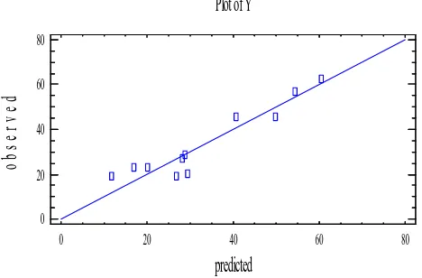
The Figures 6, 11 and 16 show the observed versus predicted plot for N5, N6 and N7 respectively. The Y axis shows the observed value of % and X axis show the predicted value by fitted model of % . It may be observed that the points are randomly scattered around the diagonal line indicating that model fits well. It may also be observed that the plot is straight line having no curve that means no need to try for higher order polynomial.

Residuals versus Predicted

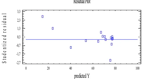
The Figures 7, 12 and 17 show of the residual analysis. The Y axis shows Studentized residual and X axis shows the predicted % from the fitted models. It may be observed that there is uniformity in variability with change in mean value shown by line in the center.

V. CONCLUSION

The models developed as shown in Table 4 for nozzles N5,

N6 and N7 to predict % by using STATGRAPHICS

considering variation with respect to , and are well fitted.

Statistical analysis showed that both factors and , have significant effect on removal efficiency ( ) but the liquid concentration is more significant between two.

ACKNOWLEDGEMENT

The author gratefully acknowledges the guidance and advice provided by Professor Vasdev Singh.

REFERENCES

1. Acharjee, D. K., Bhat, P. A., Mitra, A. K., and Roy, A. N., (1975), Studies on momentum transfer in vertical liquid jet ejectors, Indian Journal of Technology, 13, 205-210.

2. Agrawal K.S., (2013), Rate of Absorption in Laboratory Scale Jet ejector, National Journal of Applied Sciences and Engineering

Vol.1/Issue 2/July-Sept, 60-64

3. Agrawal K.S., (2012), Mathematical Model for interfacial Area for Multi Nozzle Ejector, Journal of Indian Society for Industrial and Applied Mathematics, December 2012 (Special Issue).

4. Ananthanarayanan, N. V., and Viswanathan, S., (1999), Predicting the liquid flux distribution and collection efficiency in cylindrical venturi scrubbers, Ind. Eng. Chem. Res., 38, 223-232.

5. Ananthanarayanan, N. V., and Viswanathan, S, (1998), Estimating Maximum Removal Efficiencyin Venturi Scrubbers, AIChE Journal, 44(11), 2539-2560.

6. Balamurugan, S., Gaikar, V. G., and Patwardhan, A. W., (2008), Effect of ejector configuration on hydrodynamic characteristics of gas–liquid ejectors, Chemical Engineering Science, 63, 721-731.

7. Balamurugan, S., Lad, M. D., Gaikar, V. G., and Patwardhan, A. W., (2007), Effect of geometry on mass transfer characteristics of ejectors,

Ind. Eng. Chem. Res.,46, 8505-8517.

8. Biswas, M. N., Mitra, A. K., and Roy, A. N., (1975), Studies on gas dispersion in a horizontal liquid jet ejector, Second Symposium on Jet Pumps and Ejectors and Gas Lift Techniques, Cambridge, England,

March 24-26, BHRA, E3-27-42.

9. Cramers, P. H. M. R., and Beenackers, A. A. C. M., (2001), Influence of the ejector configuration, scale and the gas density on the mass transfer characteristics of gas–liquid ejectors, Chemical Engineering Journal, 82, 131–141.

10. Cramers, P. H. M. R., Beenackers, A. A. C. M. and Van Dierendonck, L. L., (1992). Hydrodynamics and mass transfer characteristics of a loop-venturi reactor with a down flow liquid jet ejector, Chem. Engg. Sci., 47, 3557-3564.

Nozzle no.

Fitted Model R-Squared R-Squared

(adjusted for d.f.)

Standard Error of Est.

Mean absolute error

Durbin-Watson statistic

N5

= 20.6505 + 263.417

−4.09009 ± 293.901

± 16.134

86.5528 % 78.8687 % 7.69463 5.15937 1.95717

N6

= 67.9698 −99.2834

−15.4581 + 95.9406

± 17.0609

88.2783 % 80.4638 % 7.08676 4.43336 2.20699

N7

= 17.4129 + 166.782

−0.923805 ± 88.6827

± 19.0502

(10)

ISSN: 2231-5381

http://www.ijettjournal.org

Page 2940

11. Gamisansa, X., Sarrab, M., and Lafuente, F. J., (2002), Gas pollutants removal in a single and two-stage ejector venturi scrubber, Journal of Hazardous Materials, B90, 251-266.

12. Gamisans, X., Sarra, M., and Lafuente, F.J., (2004), The role of the liquid film on the mass transfer in venturi-based scrubbers, Trans IChemE,Part A, 82(A3), 372-380.

13. Li, C., and Li, Y. Z., (2011), Investigation of entrainment behavior and characteristics of gas-liquid ejectors based on CFD simulation,

Chemical Engineering Science, 66, 405–416

14. Mandal Ajay, Kundu Gautam and Mukherjee Dibyendu, (2004), Gas-holdup distribution and energy dissipation in an ejector-induced down flow bubble column: the case of non-Newtonian liquid, Chemical Engineering Science, 59, 2705 – 2713.

15. Mandal, A., Kundu, G, and Mukherjee, D., (2003b), Interfacial area and liquid-side volumetric mass transfer coefficient in a downflow bubble column, Can J of Chem Eng, 81, 212–219.

16. Mandal, A., Kundu, G. and Mukherjee, D., (2003a), Gas holdup and entrainment characteristics in a modified downflow bubble column with Newtonian and non-Newtonian liquid, Chemical Engineering and Processing, 42, 777-787.

17. Mandal, A., Kundu, G., and Mukherjee, D., (2005), A comparative study of gas holdup, bubble size distribution and interfacial area in a downflow bubble column, Trans IChemE, Part A, Chemical Engineering Research and Design, 83(A4), 423–428.

18. Mandal, A., Kundu, G., and Mukherjee, D., (2005a), Comparative study of two fluid gas-liquid flow in the ejector induced up flow and downflow bubble column, International Journal of Chemical Reactor Engineering, 3 Article A13.

19. Mandal, A., Kundu, G., and Mukherjee, D., (2005b.), Energy analysis and air entrainment in an ejector induced downflow bubble column with non-Newtonian motive fluid, Chemical Engineering Technology,

28 (2), 210-218.

20. Mukherjee, D., Biswas M. N., and Mitra, A. K., (1988), Hydrodynamics of liquid-liquid dispersion in ejectors and vertical two phase flow, Can. J. Chem. Eng., 66, 896–907.

21. Panchal, N.A., Bhutada, S.R., and Pangarkar, V.G., (1991), Gas induction and hold-up characteristics of liquid jet loop reactors using multi orifice nozzles, Chem. Engg. Communiation, 102, 59-68. 22. Ravindram Maddury and Pyla Naldu, (1986), Modeling of a venturi

scrubber for the control of gaseous pollutants, Ind. Eng. Chem. Process Des. Dev., 25(1), 35.

23. Utomo, T., Jin, Z., Rahman, M., Jeong, H. and Chung, H., (2008), Investigation on hydrodynamics and mass transfer characteristics of a gas-liquid ejector using three-dimensional CFD modeling, Journal of Mechanical Science and Technology, 22, 1821-1829.

24. Uchida, S., and Wen, C.Y., (1973), Gas absorption by alkaline solutions in a venturi scrubber, Ind. Eng. Chem. Process Des. Develop, 12 (4), 437-443.

25. Volgin, B.P., Efimova, T.F., Gofman, M.S., (1968), Absorption of sulfur dioxide by ammonium sulfite-bisulfite solutions in a venturi scrubber, International Chemical Engineering, 1 (8), 113-118. 26. Yadav, R. L., and Patwardhan, A. W., (2008), Design aspects of