Date of publication 00, 0000, date of current version 00, 0000.
Digital Object Identifier
Resample-based Ensemble Framework for
Drifting Imbalanced Data Streams
HANG ZHANG1, WEIKE LIU2, SHUO WANG3, JICHENG SHAN1, QINGBAO LIU1
1Science and Technology on Information Systems Engineering Laboratory, National University of Defense Technology, Changsha 410073, China 2College of Atmospheric Sciences, Lanzhou University, Lanzhou 730107, China
3School of Computing and Digital Technology, Birmingham City University
Corresponding author: Q. Liu ([email protected])
This study is supported by the China Advance Research Fund under Grant No. 9140C830304150C83352.
ABSTRACT Machine learning in real-world scenarios is often challenged by concept drift and class imbalance. This paper proposes a Resample-based Ensemble Framework for Drifting Imbalanced Stream (RE-DI). The ensemble framework consists of a long-term static classifier to handle gradual and multiple dynamic classifiers to handle sudden concept drift. The weights of the ensemble classifier are adjusted from two aspects. First, a time-decayed strategy decreases the weights of the dynamic classifiers to make the ensemble classifier focus more on the new concept of the data stream. Second, a novel reinforcement mechanism is proposed to increase the weights of the base classifiers that perform better on the minority class and decrease the weights of the classifiers that perform worse. A resampling buffer is used for storing instances of the minority class to balance the imbalanced distribution over time. In our experiment, we compare the proposed method with other state-of-the-art algorithms on both real-world and synthetic data streams. The results show that the proposed method achieves the best performance in terms of both the Prequential AUC and accuracy.
INDEX TERMS online ensemble learning; resample learning; reinforcement; concept drift; class imbalance
I. INTRODUCTION
With the wide application of machine learning, online learning with concept drift and class imbalance has received increased research attention. Practical applications in software engineering, risk management, traffic flows, sensor networks and social media mining face challenges of both concept drift and class imbalance [1, 2].
In a data stream, instances are generated over time based on an underlying probability distribution Pt(x,yi) [3]. If the probability distribution changes at time t, concept drift will occur. According to Bayes’ theorem [4], such drift can be divided into real concept drift and virtual concept drift. First, changes to the posterior distribution Pt(y|x) without affecting
Pt(y) will lead to real concept drift, which could change the decision boundary and decrease the performance of the classification model. Variation of the prior probability Pt(y) without affecting Pt(y|x) will lead to virtual concept drift, which changes the proportions of instances in different categories and is related to the class imbalance phenomenon.
Moreover, concept drift can be divided into sudden concept drift and gradual concept drift [5]. Sudden drift changes from an old concept to a new concept immediately, leading to a sharp decline in the classification performance. Gradual drift slowly affects the data concept, so that the classification model has an adjustment period for adapting to the new concept. If the learning algorithm focuses on only the latest instances, it will show rapid adaptability to sudden concept drift. A learning model trained by long-term instances is more conducive to handling gradual concept drift [6].
more challenging when concept drift and class imbalance occur simultaneously.
Researchers have proposed many methods to solve the joint problem of concept drift and class imbalance. According to the manner of instance arrival, the methods can be divided into block-based methods and online learning methods. Gao et al. [8, 9] first proposed Uncorrelated Bagging (UCB), which uses an ensemble method with a series of classifiers trained by a more balanced set by means of resampling the minority class and undersampling the majority class. Chen et al. [10] proposed the Selectively Recursive Approach (SERA) algorithm, which selects minority instances that are similar to those in recent data blocks. The algorithm also discards instances that are not related to the current processing block according to a distance metric. Then, the Recursive Ensemble Approach (REA) was proposed; this approach modified SERA into an ensemble approach [11]. Ditzler et al. [12] proposed Learn++.CDS and Learn++.NIE for concept drift and
class imbalance. Learn++.CDS combines the concept drift
processing algorithm Learn++.NSE [13] with the Synthetic
Minority class Oversampling TEchnique (SMOTE), which generates instances of the minority class [14]. Learn++.NIE
modifies Learn++.NSE and replaces SMOTE with
bagging-based sub-ensemble methods to address class imbalance. All the above methods are block-based algorithms which require instances to arrive in batches at each time step.
Different from block-based methods, online learning is more challenging, because only one instance is available at each time step. Online learning methods can be categorized into two main types: active handling methods that employ a drift detection mechanism [15-18] and passive methods [19, 20]. The Drift Detection Method for Online Class Imbalance (DDM-OCI) [16] is an active detection method that uses minority-class recall (i.e., true positive rate) as the indicator for concept drift. Linear Four Rates (LFR) [15] was further proposed to use the confusion matrix of the minority-class recall and precision and the majority-class recall and precision for drift detection. Additionally, many studies have evaluated indicators of classification performance. Brzezinski et al. [21, 22] modified the AUC for the online learning condition and proposed the Prequential AUC (PAUC), which can reflect the real classification performance of the minority classes, as an evaluation index. Furthermore, the Page-Hinkley test [23] uses the PAUC as the indicator and forms PAUC-PH, which can integrate other classification algorithms and actively detect drift and imbalance. However, PAUC-PH will reset and retrain the model when drift or imbalance occurs and will discard all previous knowledge.
Conversely, passive methods do not detect concept drift and class imbalance but continuously evolve the classifiers with the data stream. Many passive methods use ensemble-based methods or sampling-based methods [19, 20]. Wang et al. [20] modified the ensemble learning algorithm Online Bagging (OB) [24] and proposed Oversampling Online Bagging (OOB) and Undersampling Online Bagging (UOB). These methods
calculate the real-time size of classes to evaluate the current imbalance degree for determining the sampling times of instances. Moreover, a time decay factor is used to decrease the impact of historical data. DDM-OCI, LRF, PAUC-PH, OOB and UOB are designed for binary classification, which defines two classes: minority and majority.
Generally, block-based learning methods learn fixed-size data blocks and respond inefficiently to sudden concept drift which happens within a data block. Although reducing the size of the data blocks can help to address sudden drift, this change increases the computational cost and degrades the performance in the stable state [6]. In contrast to the block-based methods, online learning models are dynamically updated by new arriving instances and can rapidly adapt to sudden concept drift. However, they may perform quite poorly at the initial stage of training compared to block-based ones, because only one instance is used at each time step. Therefore, in this proposal, we are motivated to combine the advantages of block-based and online learning. The component classifiers in our ensemble method are created by a block-based method and the instances are processed in an online manner.
In this paper, we propose a novel resample-based ensemble framework for a drifting data stream with class imbalance (RE-DI). The novelty lies in the following aspect. First, we proposed a novel ensemble framework that includes a long-term static classifier and multiple dynamic classifiers using a sliding window. The static classifier is maintained and updated throughout the entire learning procedure to handle gradual changes in the data stream. The dynamic classifiers learn only recently received data and are more suitable for addressing sudden concept drift. Second, the classifier weights are dynamically adjusted by two approaches. A novel reinforcement mechanism dynamically adjusts the predictive weights of the base classifiers and improves the classification performance for the minority class. Older dynamic classifiers have their weights periodically decreased, so that the final ensemble model can focus on the latest concept of the data stream. Third, to balance the imbalance ratio of training samples, a resample-based initialization method for base classifiers is proposed. It uses a resampling buffer group to store and supply instances of the minority class.
The rest of this paper is organized as follows. The resample-based ensemble framework for drifting imbalance stream is proposed in Section 2. Section 3 present the experimental results and analysis, and the conclusions are presented in Section 4.
II. METHODS
initialization procedure for a base classifier that aims at solving the learning problem posed by class imbalance. First, we introduce the structure of the resample-based ensemble framework.
Cs C1 CD-1 CD
…… ……
Dynamic Classifier Sliding Window
Ensemble Classifier E
Supply training samples
Resampling Buffer Group U
… …
… ……
U[1]
Data Stream ……
…… …… ……
……
I instances 2I instances
…… ……
…… …………
The whole stream
Bn Bn-1
B1
U[2] U[L] Static Classifier
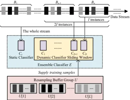
Figure 1. Structure of resample-based ensemble framework
As shown in Figure 1, the ensemble classifier E consists of a static classifier Cs and D dynamic classifiers Cd (d = 1, 2, …,
D). The D dynamic classifiers are periodically created and replaced. Additionally, the resampling buffer group is used for supplying training samples of the minority class. As the class imbalance ratio could vary and the minority class can change into the majority class, all L categories have a corresponding resampling buffer.
A. ENSEMBLE LEARNING PROCEDURE
Tradition block-based learning algorithms create base classifiers and make predictions in the units of a fixed-size data block. The classifiers are trained on the current data blocks and make predictions on subsequent data blocks. However, concept drift can occur at any point in the data stream. Therefore, if concept drift occurs within a data block, block-based learning methods will have a delay in adapting to concept drift. Online learning addresses the newly arriving instances one by one and can rapidly respond to the changes in data stream. However, the block-based learning algorithm will have more training samples for initializing a new classifier. Additionally, in the resample-based ensemble framework, dynamic classifiers are dynamically created and replaced. Each dynamic classifier only exists for a period. Therefore, the component classifiers in the ensemble framework are created by a block-based method, and instances in the data stream are processed in an online learning manner. Let S be an infinite data stream …, xi, xi+1, xi+2, …. At time
t, the arriving instance is xt and the class label of xt is yt. A circular cache array B is used to cache instances from the data stream and form data blocks. In addition, the length of the circular cache array B is I. Therefore, the data stream can be regarded as a consequent data block queue B1, B2, … Bn,
Bn+1 …. Algorithm 1 shows the ensemble learning procedure
of the proposed methods.
Algorithm 1
EnsembleLearning Procedure
Inputs:
1. S: data stream with unknown label 2. L: number of classes
3. I: size of the data blocks
4. D: number of dynamic classifiers
5. ɛ: instance selection ratio of the classifier initialization.
Output: Ensemble Classifier E
Initialization:
1. B: circular cache array, initialized as an empty array 2. U[l]: resampling buffer for storing instances 3. p=0: counter of processed instances
4. i=0: indicator of current position in circular cache array 5. k=0: indicator of the dynamic classifiers
Process:
1. while (S. hasNext()) do
2. xnew=S. nextInstance() 3. p=p+1
4. if (p<I) then // Before B is fully filled for the first time 5. B[p-1]=xnew
6. elseif (p==I) then // Fill the array for the first time 7. B[p-1]=xnew
8. Cs=CreateNewBaseClassifier(ε,U,I,L,D,wd,ws,DCIR[l]) //Create static classifier
9. k=1
10. C1=Cs // Create the first dynamic classifier 11. else // (p>I) has more instances than I
12. i=(p-1)%I // i is the current index for A
13. TrainOnInstance (xnew,i,L,D,wd,ws,DCIR[l]) 14. i=(i+1)%I // i moves circularly 15. if (i==0) then // The array is filled again 16. k=k+1
17. Ck=CreateNewBaseClassifier(ε,U,I,L,D,wd,ws,DCIR[l]) //create new dynamic classifier
18. if (k>D) then
19. CdCd+1 (d=1, …, D-1)
20. CDCk 21. endif
22. Update the predictive weight of classifiers by (3) 23. Calculate damped class imbalance ratio by (5) 24. endif
25. endif
26. endwhile
27. for i=0 to I-1 do // Address remaining instances 28. xnew=B[i]
29. TrainOnInstance (xnew,i,L,D,wd,ws,DCIR[l]) 30. end for
After the learning process begins, the circular array B
continuously caches arriving instances from the data stream until it is filled for the first time. When the circular array is filled for the first time, the first data block B1 is used to create
instances in the circular array are learned one by one. The learning process starts from the first position in the circular cache array, and an indicator i is used to represent the current processing position. The procedure for training on an instance is shown in Algorithm 2.
Algorithm 2
TrainOnInstance(xnew,i,L,D,wd,ws,DCIR[l]) Inputs:
1. xnew: new instance from data stream
2. i: current processing position of the data block 3. L: number of classes
4. D: number of dynamic classifiers 5. ws: weight of static classifier
6. wd: weights of dynamic classifiers (d=1, …, D) 7. DCIR[l]: damped class imbalance ratio
Output: Adjusted weights ws and wd (d=1, …, D) Process:
1. xi=B[i] //get instance from the circular cache array 2. ReinforcementWeightAdjustment(xi,L,D,wd,ws,DCIR[l]) 3. update the static classifier and dynamic classifiers with xi 4. B[i]= xnew //cache the new instance xnew
First, instance xiis obtained from the circular cache array
B[i]. Then, the reinforcement weight adjustment mechanism (Algorithm 3) is used to improve the classification performance of the ensemble framework for the minority class. Then, the static classifier and dynamic classifiers are trained using xi. Once the instance in position i is learned, the instance is replaced by the newly arriving instance xnew, and the indicator moves to the next position in the circular cache array. When indicator i reaches the last position, all the instances in the cache array have been replaced, meaning that a new data block is formed. Then, the indicator moves to the first place and the algorithm will learns from the new data block from the beginning.
When a new data block is formed, the algorithm creates a new dynamic classifier Cnew in the ensemble. As the learning procedure proceeds, the number of classifiers in the ensemble framework continues to grow. If the number of classifiers exceeds D, the earliest dynamic classifier C1 is dropped. Then,
the subsequent classifier will replace the former classifiers one by one Cd←Cd+1 (d = 1, …, D−1) to ensure that there are
always D classifiers in the ensemble framework. Next, the weights of the dynamic classifiers are updated according to (3), and the damped class imbalance ratio is calculated by (5). Finally, when no more instance can be obtained from the data stream, the algorithm learns the remaining instances in the cache array.
B. ENSEMBLE FRAMEWORK WITH REINFORCEMENT
ADJUSTED AND TIME-DECAYED WEIGHT
In this section, the ensemble framework with reinforcement-adjusted weight is introduced. The ensemble classifier consists of a static classifier and a dynamic classifier sliding window. To handle the long-term tendency of the data stream, the static classifier Cs learns the whole data stream while the dynamic
classifiers Cd learn only a part of the data stream, which is defined as:
⎩ ⎪ ⎨ ⎪
⎧S
s= Bk n
k=1
Sd= Bn-D+k D
k=d
, d=1, 2,… D
(1)
Suppose the current processed data block is Bn, the data stream learned by the static classifier is Ss and the parts learned by the dynamic classifier are Sd. The dynamic classifier Cd, learns only the most recent D-d+1 data blocks of the data stream. Each dynamic classifier exists for only a period of time and is replaced by the newly created dynamic classifier. The joint prediction of the ensemble classifier is the weighted combination of the static classifier and dynamic classifiers, is calculated as follows:
f lE(x)=ωsf l
Cs(x)+ ωdf l Cd(x) D
d=1
,l=1,…L (2)
f lE(x) is the ensemble prediction that instance x belongs to class l. ws and wd (d = 1, …, D) are the predictive weights of the static classifier and dynamic classifiers. The weight of the static classifier ws is initialized to 0.5, and the weights of the dynamic classifiers wd decrease over time. Whenever a new dynamic classifier is created, its initial weight is set to 1/D, and the weights of the old dynamic classifiers are reduced repeatedly over time, as shown in Equation (3). Then, the weights of all the classifiers are normalized
⎩ ⎪ ⎨ ⎪ ⎧ωs←1
2
ωd←ωd(1-1
D) ωD←1
D
,d=1, 2,… D-1 (3)
Through dynamic weight attenuation, the newly created dynamic classifier is given more weight than the older classifiers in the joint prediction. Therefore, the algorithm will focus more on the latest instances, which will help to adapt to concept changes in the data stream. Additionally, in the class imbalanced learning condition, the classification performance on the minority class should be given more attention. The data stream learned by each dynamic classifier is different, so the classification capacity for the minority category of the dynamic classifiers is different. Therefore, to improve the joint prediction accuracy of the ensemble classifier for the minority class, a reinforcement weight adjustment mechanism is proposed in Algorithm 3.
Algorithm 3
ReinforcementWeightAdjustment(x,L,D,wd,ws,DCIR[l]) Inputs:
1. x: processed instance of label y
2. L: number of classes
3. D: number of dynamic classifiers 4. ws: weight of static classifier
6. DCIR[l]: damped class imbalance ratio
Output: Adjusted weights ws and wd (d=1, …, D) Process:
1. if (DCIR[y]<1/L) then // if instance x belongs to the minority class
2. ford=1 toDdo:
3. if (Predictright(x, Cd)==True) then //Cd predicts right 4. wd= wd*(1+1/D) // increase weight of Cd
5. else
6. wd= wd*(1-1/D) // decrease weight of Cd 7. end if
8. end for
9. if (Predictright(x, Cs)==True) then //Cs predicts right 10. ws= ws*(1+1/D) // increase weight of Cs
11. else
12. ws= ws*(1-1/D) // decrease weight of Cs 13. end if
14. end if
First, for arrival instance x of class y, the algorithm determines whether instance x belongs to the minority class according to the Damped Class Imbalance Ratio (DCIR). Then, if x is in the minority class, the prediction results of the static classifier and dynamic classifiers are used as the foundation for adjusting the weights. That is, if a classifier correctly predicts the class label of x, the weight of this classifier is increased by (1+1/D). Otherwise, weight wd is decreased by (1-1/D). Therefore, classifiers that perform better on the minority class are given more weight in the ensemble prediction.
In sum, the ensemble classifier with reinforcement-adjusted weight makes the following efforts to address concept drift and class imbalance. To deal with the different types of concept drift, the ensemble framework includes a long-term static classifier and multiple dynamic classifiers. The static classifier in the ensemble framework is used throughout the entire learning procedure, which helps to handle gradual concept change. Then, the dynamic classifiers use a sliding window [25] structure to learn partial data streams and enable rapid adaptability to sudden concept drift. The weight adjustment strategy contributes in two aspects. On the one hand, the weights of the dynamic classifiers are decreased over time to make the ensemble classifier focus more on the new concept of the data stream. On the other hand, the reinforcement mechanism selectively adjusts the weights of the static classifier and dynamic classifiers, improving the overall classification performance of the ensemble classifier E
for the minority class.
C. RESAMPLE-BASED INITIALIZATION FOR BASE CLASSIFIER
In the scenario where the data stream is class imbalanced, the learning model will lack training samples of the minority class because of the biased class distribution. Many block-based methods [9, 10, 12] apply random sampling or smart sampling techniques to form class-balanced training sets. However, if
concept drift occurs, these sampling methods could select instances of the old concepts that will lower the classification performance. These sampling methods thus cannot be used in online learning conditions. OOB and UOB [20] integrate oversampling and undersampling methods into online bagging which train more times with the minority class or train fewer times with the majority class. The component classifiers in online bagging address all the instances throughout the entire learning procedure, but in our proposed ensemble, the dynamic classifier only exists for a certain period and learns a partial data stream. There is no guarantee that the dynamic classifier can obtain enough instances of the minority class in its corresponding partial data stream. Therefore, in this section, a resample-based initialization method for base classifiers is proposed to solve this problem by improving the classification capacity for the minority class during the initialization process of the base classifiers.
As the class imbalance condition of the data stream could change over time, the minority class and majority class may transform into each other. Therefore, for each category l, a resampling buffer U[l] (l = 1, …, L) (pink rectangle) is used to cache instances of this class. Whenever the ensemble classifier addresses an instance, it stores the instance in the corresponding resampling buffer by class label. Instances are stored in order and the later arriving instances are used first. In addition, the length of the resampling buffer is periodically reduced to save memory and discard old instances. The resample-based initialization procedure for the base classifiers is shown in Algorithm 4.
Algorithm 4
CreateNewBaseClassifier(ε,U,I,L,D,wd,ws,DCIR[l]) Input:
1. ε: instance selection ratio 2. U: resampling buffer 3. I: size of data block 4. L: number of classes
5. D: number of dynamic classifiers
6. wd: weights of dynamic classifiers (d=1, …, D) 7. DCIR[l]: damped class imbalance ratio
Output: A new classifier Cnew Process
1. Select the top εI instances of current block Bn to form the initialization set Rn
2. fori=0 toIε-1 do: 3. xi=Rn[i]
4. ReinforcementWeightAdjustment(xi,L,D,wd,ws,DCIR[l]) 5. end for
6. Calculate instance numbers Hn[l] of different classes in
Rn
7. Create the classifier Cnew
8. For each class l, if Hn[l] < I*ε/L, use the most recent I*ε/L
- Hn[l] instance in U[l] to train Cnew 9. Use Rn to train Cnew
11. Reduce the length of all resampling buffers U[l] to I*ε/L
12. Return Cnew
Whenever a new data block arrives, a new classifier is created. Assume that the current processing data block is Bn. First, the algorithm uses the top εI instances of the current block Bn and forms an initialized dataset Rn. Then, for each instance in Rn, the reinforcement mechanism is used to adjust the predictive weights of the classifiers in the ensemble framework. Then, the numbers of instances in different categories Hn[l] in the initialized dataset Rn are calculated. To balance the training samples of the different classes, instances in the resampling buffer are used according to (4).
𝐻 (𝑙) <𝜀𝐼
𝐿, 𝑆ℎ𝑜𝑟𝑡𝑎𝑔𝑒
𝐻 (𝑙) ≥𝜀𝐼
𝐿, 𝐸𝑛𝑜𝑢𝑔ℎ
(4)
Define ɛ as the instance selection ratio. I is the size of the data block, and L is the number of classes. To ensure that the classifier can obtain enough instances of the minority class, set
ɛI/L as the minimum quantity of instances for each category to initialize the new classifier. For each class l, if Hn(l) is smaller than ɛI/L, the new classifier Cnew will be updated by the most recent I*ε/L - Hn[l]instances from the resampling buffer U[l], otherwise, Cnew has trained on enough instances of class l. Finally, use Rn to update Cnew. Furthermore, instances from Rn are stored in the corresponding resampling buffer by class label. Finally, the length of all the resampling buffers is reduced to ɛI/L, which is the maximum quantity needed by the resampling procedure.
To evaluate the class imbalance degree of the data stream, the damped class imbalance ratio (DCIR) is proposed. For all the dynamic classifiers that exist in the ensemble classifier, each classifier has a corresponding initialization dataset Rd. The class distribution Hd(l) of Rdis also calculated. Then the damped class imbalance ratio is:
DCIR(l)= ∑ Hd[l]w
d D
d=1
∑1l=0∑Dd=1Hd[l]wd
(5)
wdis the predictive weight of classifier Cd calculated in (3). For each class l, the weighted summation of the instances including all the initialization dataset Rd is calculated. DCIR(l) is the ratio of category l to the summation of all the categories. As wd decays with time, the older class distribution information has less effect in calculating DCIR, which helps the algorithm focus on the most recent class imbalance ratio of the data stream.
III. EXPERIMENTS
In this section, the performance of RE-DI is compared with that of the other state-of-the-art methods, including OOB, UOB, LB and ARF. First are three modification methods of online bagging. OOB and UOB [20] integrate sampling methods in online bagging for class imbalance learning. Leveraging Bagging (LB) [26] which modifies online bagging by adding more randomization in the ensemble is also compared. In addition, the most recent learning method for an
evolving data stream, Adaptive Random Forests (ARF) [27] is also included.
All the algorithms are implemented in the MOA data stream software suite [28]. All the algorithms will first test on the arriving instance and then train on it. Particularly, RE-DI has its own task function to realize the special learning procedure that combines the block-based and online learning methods, and the other methods use the prequential evaluation settings in MOA. To maintain the consistent performance of the base classifier, all the comparative methods except ARF, apply the Hoeffding Tree as the base classifier. The Hoeffding Tree is an incremental, anytime decision tree induction algorithm that is capable of learning from massive data streams. And it was wildly used as base classifier in researches of online data stream learning. ARF uses ARFHoeffding which is specifically designed for this algorithm as the base classifier. It is worth mentioning that RE-DI can use other classifiers provided by MOA as the base classifier of the ensemble. Moreover, all the experiments are carried out on a machine with an eight-core Intel i7-6700 CPU, 3.4 GHz processor, and 32 GB of RAM.
Section A to E present the results of comparing RE-DI with other state-of-the-art methods. In section F, a verification experiment is designed and carried out to prove the effect of the static classifier and dynamic classifiers in the ensemble framework.
A. DATA STREAMS
In the experimental evaluation, we used both synthetic data streams and real data streams to compare the performance of the algorithms in different situations. The default parameters of RE-DI are D=10, I=500, and ε=0.20. For each dataset, we conducted five parallel experiments on all the data streams. To evaluate the performance of algorithms in a specific condition of a data stream, we chose the synthetic generators in MOA, Agrawal and HYP to generate synthetic datasets. In addition, to verify the practicability in real-word applications, we also used real-world data streams.
Agrawal is used to generate data streams with sudden concept drift and class imbalance. The different functions of the generators simulate various concepts of data streams. When a sudden concept drift occurs, the generation function changes within 25 instances. First, data streams with a fixed class imbalance ratio and sudden concept drift (Agrawal37,
Agrawal28, Agrawal19) are generated. Then, a data stream with
For the real data streams, we chose four commonly used data streams as benchmarks, PAKDD [21], Give Me Some Credit (GMSC), Forest Covertype (Covtype) [27] and poker. PAKDD predicts credit card fraud cases from a large amount of transaction records. GMSC is a credit scoring data stream which is used for risk assessment in loan. PAKDD and GMSC are binary data streams which can be used directly. For the multi-class data streams, the same approach in [9] which selects one category as the majority and another as the minority, is applied to convert the data streams to binary streams. Covtype contains the forest cover type for 30x30
meter cells obtained from US Forest Service (USFS) Region 2 Resource Information System (RIS) data. Covtype contains 581, 012 instances, 54 predictive attributes and 7 classes from 1 to 7. In covtype36, class 3 is used as the majority and class 6 is the minority. Poker consists of 10 predictive attributes and 10 classes. Each record of Poker is an example of a hand consisting of five playing cards drawn from a standard deck. Poker23 selects class 2 as the majority and class 3 as the minority. Table I summarizes the main characteristics of the experimental data streams.
TABLEI
CHARACTERISTICOFDATASTREAMS
Data stream No. Inst No. Attrs Class Class ratio Drift Type No. Drifts
covtype36 53 k 54 2 1/2 - -
PAKDD 50 k 28 2 1/4 - -
poker23 390 k 10 2 1/9 - -
GMSC 150 k 10 2 1/14 - -
Agrawal37 100 k 9 2 3/7 sudden 3
Agrawal28 100 k 9 2 2/8 sudden 3
Agrawal19 100 k 9 2 1/9 sudden 3
AgrawalRS 100 k 9 2 3/7,2/8,1/9,3/7 sudden 3
HYP37 100 k 5 2 3/7 gradual 1
HYP28 100 k 5 2 2/8 gradual 1
HYP19 100 k 5 2 1/9 gradual 1
HYPRG 100 k 5 2 1/1,1/9 gradual 1
TABLEⅡ
AVERAGEAUC(%)WITHDIFFERENTNUMBEROFDYNAMICCLASSIFIERS,BLOCKSIZEANDINSTANCESELECTIONRATIO
Data stream 1 5 10 D 15 20 100 250 500 I 750 1000 0.05 0.1 0.15 ε 0.2 0.25
covtype36 96.7 98.4 98.6 98.6 98.6 98.3 98.6 98.6 98.5 98.2 97.9 98.3 98.5 98.6 98.7
PAKDD 60.0 63.9 65.8 66.5 67.0 65.4 65.4 65.8 65.4 65.8 63.0 63.9 64.9 65.8 66.7
poker23 95.5 97.3 97.9 98.2 98.4 95.9 96.6 97.9 97.1 97.9 96.7 96.8 98.0 97.9 97.7
GMSC 77.2 83.5 85.2 85.8 86.1 83.4 84.6 85.2 85.3 85.1 83.6 83.9 84.6 85.2 85.9
Agrawal37 85.0 93.7 94.6 94.7 94.7 91.7 89.1 94.6 93.7 93.6 90.3 89.2 91.0 94.6 94.9
Agrawal28 76.8 88.6 90.3 90.8 91.0 86.3 88.0 90.3 91.1 90.7 88.6 88.2 90.1 90.3 91.0
Agrawal19 70.0 84.1 86.9 87.9 88.5 81.9 85.1 86.9 86.8 86.8 85.2 84.6 85.2 86.9 87.8
AgrawalRS 87.0 93.0 94.0 94.2 94.2 91.5 88.6 94.0 92.8 93.4 89.1 88.5 90.0 94.0 93.5
HYP37 98.5 99.3 99.4 99.5 99.5 99.2 99.4 99.4 99.4 99.4 99.4 99.4 99.4 99.4 99.4
HYP28 97.3 98.9 99.1 99.1 99.2 98.7 99.0 99.1 99.1 99.1 99.0 99.0 99.0 99.1 99.1
HYP19 95.8 98.0 98.4 98.5 98.6 97.8 98.4 98.4 98.6 98.5 98.2 98.3 98.3 98.4 98.5
HYPRG 96.5 98.3 98.5 98.5 98.5 98.1 98.4 98.5 98.5 98.3 98.3 98.3 98.5 98.5 98.6
B. EVALUATION INDICATOR
Traditional classification performance evaluation methods use accuracy as the indicator. However, accuracy reflects only the overall performance on all categories, when the accuracy of the minority class is poor, the overall accuracy is still high. AUC calculates the area under the ROC curve and is a suitable metric for evaluating class imbalance learning. However, AUC can be used in only offline learning condition. Recently, many works [21, 22] have modified AUC for online learning conditions and propose Prequential AUC (PAUC). Therefore, we applied Prequential AUC as the experimental evaluation indicator. Additionally, we compared the PAUC indicator with the traditional accuracy indicator.
C. PARAMETER SENSITIVITY
In this section, to verify the parameter sensitivity of RE-DI, we performed parameter comparison experiments on the main
setting parameters, including the number of dynamic classifiers D, the size of the data blocks I, and the instance selection ratio ε. The default values are D=10, I=500, and
ε=0.20. For each parameter, we conducted five parallel experiments on all the data streams.
From Table Ⅱ, we can see that all the parameters have an impaction on the classification performance of RE-DI. First, within the parameters selected for the experiments, the number of dynamic classifiers is positively correlated with the classification performance. Second, RE-DI performs better at block sizes of 500 and 750, which shows that the best optimal block size parameter is determined by the experimental data stream. At last, the classification performance is improved when the algorithm uses more instances during the initialization process. Intuitively, the higher instance selection ratio can help the new classifier acquire a more detailed understanding of the current data stream.
TABLE Ⅲ
Data stream RE-DI AUC Acc. PAUC-OOB AUC Acc. PAUC-UOB AUC Acc. PAUC-LB AUC Acc. PAUC-ARF AUC Acc.
1 covtype36 98.6 95.1 69.9 68.0 74.2 69.1 98.5 95.1 97.7 92.5
2 PAKDD 65.8 80.3 63.5 70.7 60.7 42.4 62.6 79.9 63.2 80.1
3 poker23 97.9 95.1 71.7 87.6 68.4 58.9 98.0 96.7 93.5 93.5
4 GMSC 85.2 93.6 84.9 89.7 71.2 93.0 81.9 93.5 80.4 93.5
5 Real Avg 86.9 91.0 72.5 79.0 68.6 65.6 85.3 91.3 83.7 89.9
6 Real Avg Rank 1.25 1.38 4.50 4.50 4.75 4.50 2.50 2.00 3.25 2.62
7 Agrawal37 94.6 88.7 84.2 71.5 74.1 67.1 85.7 81.6 87.5 81.3
8 Agrawal28 90.3 87.2 85.4 76.4 73.6 66.9 81.7 84.8 87.0 84.3
9 Agrawal19 86.9 91.4 84.8 84.9 73.1 67.3 77.0 91.0 82.3 90.4
10 AgrawalRS 94.0 89.5 84.2 72.2 74.4 65.3 82.0 83.5 85.6 84.1
11 HYP37 99.4 96.5 99.1 95.1 97.4 90.7 99.1 95.4 98.9 95.0
12 HYP28 99.1 95.8 98.6 94.3 95.8 87.2 98.5 94.9 98.4 94.5
13 HYP19 98.4 96.9 96.1 92.4 90.9 82.1 97.5 96.4 97.3 95.9
14 HYPRG 98.5 95.2 95.3 89.1 83.9 75.0 97.0 93.4 96.9 93.1
15 Synthetic Avg 91.5 92.7 85.8 84.5 80.4 75.2 83.1 90.1 88.7 89.8
16 Synthetic Avg Rank 1.00 1.00 3.00 3.88 5.00 5.00 3.12 2.12 2.88 3.00
17 Overall Avg 92.4 92.1 84.8 82.7 78.2 72.1 88.3 90.5 89.1 89.9
18 Overall Avg Rank 1.08 1.12 3.08 4.08 4.92 4.83 2.92 2.08 3.00 2.88
D. COMPARATIVE STUDY ON DATA STREAMS
In this section, the performance of the algorithms on different data streams is compared. RE-DI was compared with PAUC-OOB, PAUC-UOB, PAUC-LB and PAUC-ARF. All the comparison methods are ensemble methods, and the experiments were conducted 5 times independently. Table Ⅲ shows the average AUC (%) and average Accuracy (%) of the algorithms on all data streams.
First, the performance of the data streams with sudden concept drift and class imbalance, which are generated by Agrawal (Agrawal37, Agrawal28, Agrawal19, AgrawalRS) are compared. RE-DI achieves the highest AUC and accuracy value compared with the other methods on these data streams. As the class imbalance ratio increases, the AUC value decreases because of the growing classification difficulty on the minority class. However, the classification accuracy on Agrawal19 is higher than that on Agrawal37, Agrawal28 or
AgrawalRS. This phenomenon agrees with the previous analysis of class imbalance learning, as even when the overall classification accuracy is high, the classification performance on the minority class could be poor. The AUC indicator, however, can reflect the real classification performance on the minority class.
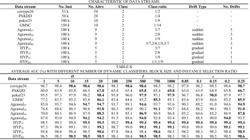
Figure 2 shows the average AUC curve and average accuracy curve of Agrawal37 and the dotted lines divide the
concepts and imbalance ratios at different stages in the data stream. When concept drift occurs, the AUC curve of RE-DI first decreases and then tends to be stable or rise. When the learning procedure ends, RE-DI has a clear lead over the other algorithms. Additionally, when the learning procedure begins, RE-DI and PAUC-UOB show a high initial AUC values, reflecting the fast adaptability of the algorithms. However, the AUC value of PAUC-UOB rapidly decreases at the first and second concept drifts, and it performs the worst at the end. Conversely, PAUC-ARF and PAUC-LB have better drift adaptive capacities than PAUC-UOB. Therefore, they perform better than PAUC-UOB at the end. In general, it can
be concluded from the analysis of the curve that RE-DI has the best overall adaptability among all the algorithms.
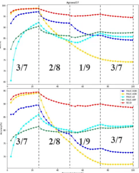
Figure 2.Classification AUC (%) and Accuracy (%) on Agrawal37 Then, the performance of the data streams with gradual concept drift and class imbalance that are generated by HYP are analyzed (HYP37, HYP28, HYP19, HYPRG). RE-DI achieves the best classification AUC and classification accuracy on all data streams. For the data streams with a fixed class imbalance ratio, the classification AUC decreases as the class imbalance ratio increases.
performance on both the classification AUC and classification accuracy during the whole learning process. As opposed to with the data stream with sudden concept drift, there is no upward or downward trend on the data stream with gradual concept drift. The classification AUC curves of most algorithms except for PAUC-UOB keep rising since the beginning of the learning procedure and remain stable in the second half of the learning process.
Figure 3.Classification AUC (%) and Accuracy (%) on HYPRG
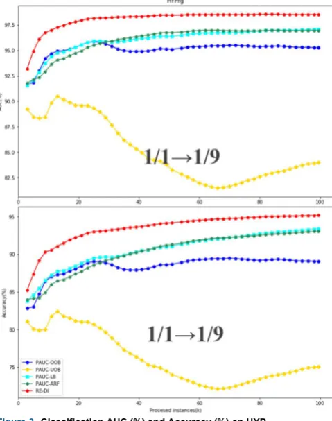
At last, a comparative experiment is performed on real-world data streams whose concept drift condition is unknown.RE-DI achieves the best AUC performance on most of the real-world data streams. For poker23, RE-DI takes the second place on the AUC and accuracy indicators and PAUC-LB achieves the first place. Although accuracy of RE-DI is 1.6% lower than that of PAUC-LB, the difference in AUC value is only 0.1%. It can be concluded that RE-DI has better classification capacity on the minority class than PAUC-LB. Figure 4 shows the average AUC curve and average accuracy curve of the real-word data stream PAKDD. Although the classification accuracies of RE-DI, LB and PAUC-ARF are approximatively equal, the AUC of RE-DI is higher than that of PAUC- LB or PAUC- ARF. The accuracy of OOB is much lower than that of LB or PAUC-ARF, but it still has a higher AUC value because of the better performance on the minority class.
Figure 4.Classification AUC (%) and Accuracy (%) on PAKDD
In addition, a statistical test [29] on the classification AUC and accuracy of different methods on all the data streams is carried out. Concretely, the statistical test is conducted on both real-world data streams (Line 6 in Table Ⅲ) and synthetic data streams (Line 16 in Table Ⅲ). And the overall results on both synthetic and real-world data streams are shown in Line 18 in Table Ⅲ. RE-DI achieves the first place in the ranking for both AUC and accuracy indicators. Then, the Nemenyi post-hoc test is used to identify the difference between the algorithms, and the results are plotted in Figure 5 and Figure 6. The statistical test on the accuracy value indicates that there is no significant difference between RE-DI, LB, and PAUC-ARF. However, in the statistical tests on the AUC indicator, RE-DI is better than the other methods.
Figure 5. Nemenyi test with 95% confidence level on AUC
TABLEⅣ
AVERAGETIME(CPU-SECONDS)ANDRAM(RAM-HOURS)OFDIFFERENTALGORITHMS
Data stream RE-DI PAUC-OOB PAUC-UOB PAUC-LB PAUC-ARF
Time RAM Time RAM Time RAM Time RAM Time RAM
1 covtype36 16.9 4.9E-06 4.7 3.1E-07 3.9 2.6E-07 43.4 1.1E-04 11.3 4.4E-06
2 PAKDD 9.2 2.0E-06 6.5 4.0E-06 2.7 1.3E-07 102.7 1.4E-03 28.9 1.3E-04
3 poker23 44.1 3.0E-06 21.7 7.0E-07 17.0 5.5E-07 132.7 2.0E-04 60.5 2.2E-05
4 GMSC 13.2 1.3E-06 14.6 1.1E-05 4.9 1.6E-07 157.9 1.3E-03 68.7 3.4E-04
5 Real Avg 20.9 2.8E-06 11.9 4.0E-06 7.7 2.8E-07 109.2 7.5E-04 42.4 1.3E-04
6 Real Avg Rank 3.00 2.75 2.25 2.50 1.00 1.00 5.00 5.00 3.75 3.75
7 Agrawal37 11.5 2.2E-06 22.1 5.1E-05 3.4 1.1E-07 61.9 2.4E-04 56.7 2.4E-04
8 Agrawal28 10.9 1.9E-06 27.5 7.9E-05 3.2 9.8E-08 67.3 2.9E-04 49.0 1.8E-04
9 Agrawal19 9.9 1.6E-06 25.4 6.0E-05 3.1 9.3E-08 55.4 1.8E-04 65.1 3.5E-04
10 AgrawalRS 11.1 2.1E-06 24.5 6.3E-05 3.3 1.0E-07 71.2 3.4E-04 53.8 2.2E-04
11 HYP37 6.3 3.8E-07 5.4 1.3E-06 2.6 6.7E-08 37.9 1.0E-04 13.9 1.2E-05
12 HYP28 6.9 4.4E-07 7.7 3.5E-06 2.6 6.5E-08 43.3 1.4E-04 17.5 2.0E-05
13 HYP19 6.4 3.7E-07 6.9 2.6E-06 2.4 6.1E-08 25.8 4.3E-05 15.6 1.8E-05
14 HYPRG 6.8 4.2E-07 7.2 2.8E-06 2.5 6.4E-08 36.5 8.7E-05 16.2 1.6E-05
15 Synthetic Avg 8.7 1.2E-06 15.9 3.3E-05 2.9 8.2E-08 49.9 1.8E-04 36.0 1.3E-04
16 Synthetic Avg Rank 2.12 2.00 2.88 3.00 1.00 1.00 4.88 4.75 4.12 4.25
17 Overall Avg 12.8 1.7E-06 14.5 2.3E-05 4.3 1.5E-07 69.7 3.7E-04 38.1 1.3E-04
18 Overall Avg Rank 2.42 2.25 2.67 2.83 1.00 1.00 4.92 4.83 4.00 4.08
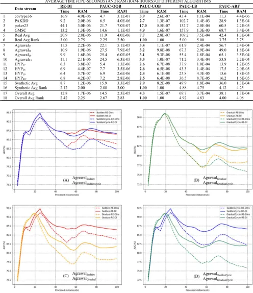
Figure 7.AUC curves of RE-DI and RE-DINS on comparative data streams
E. RESOURCES COMPARISON
In this section, the average memory and processing time of the comparative algorithms on all data streams are compared. Table 4 shows the average time (CPU-seconds) and RAM
(RAM-hours) cost of the algorithms on all data streams. And the statistical test is also carried out.
time and memory. Analysis from the algorithm level, OOB resample the instances of the minority class but PAUC-UOB undersampling the instances of the majority class. As the class imbalance ratio increases, PAUC-UOB will cost less resource on instances of the majority class and PAUC-OOB will cost more resource on instances of the minority class. RE-DI solves the class imbalance problem by supplying limited number of the minority instances, so the changing in class imbalance ratio will not obviously influence its resource consuming.
F. VERIFICATION OF THE PROPOSED FRAMEWORK To deal with different types of concept drift, RE-DI includes a static classifier and multiple dynamic classifiers. The static classifier learns the entire data stream throughout the learning process, which is more suitable for handing gradual drift. However, dynamic classifiers only exist for a certain period and learn only part of the data stream. If sudden drift occurs, the dynamic classifiers can more easily adapt to the changes. In addition, the static classifier contains more historical knowledge of the data stream compared with the dynamic classifier. For data streams with a cyclic concept drift in which an old concept shows up again, the static classifier with historical knowledge will easily adapt to the reoccurring concept.
TABLEⅤ
AVERAGEAUC(%)ANDACCURACY(%)OFRE-DIANDRE-DINS
Data stream RE-DI RE-DINS
AUC Acc. AUC Acc.
AgrawalSudden 86.5 91.4 83.9 91.1
AgrawalSuddenCycle 86.7 91.0 82.4 90.6
AgrawalGradual 81.7 90.8 78.3 90.7
AgrawalGradualCycle 82.0 90.5 76.0 90.3
Avg 84.5 90.9 80.2 90.7
In this section, to verify the rationality and necessity of the static classifier, comparative experiments between the original RE-DI and RE-DINS are carried out. RE-DINS only has dynamic classifiers in the ensemble framework. The Agrawal generator is used to generate four types of data streams AgrawalSudden, AgrawalSuddenCycle, AgrawalGradual, AgrawalGradualCycle. All these data streams have concept drifts that occur at the 1/4, 2/4 and 3/4 positions of the data stream. For the data stream with subscript Sudden, the width of concept change is set to 1, while the width of Gradual stream is 10000. The Agrawal generator has ten functions for producing instances and each function is used to represent a concept. Concretely, the data streams with subscript Cycle use two functions and have cyclic concept drift (Functions: 1/2/1/2), while the data streams without subscript Cycle use four functions (Functions: 1/2/3/4). Table Ⅴ shows the experimental results of RE-DI and RE-DINS. On all the data streams, RE-DI is better than RE-DINS. Furthermore, to reflect the adaptive ability of the static classifier to the cyclic concept drift and gradual concept drift, the types of concept drift are used as the control variables to paint Figure 7.
In Figure 7, each color represents the result on a data stream (red: AgrawalSudden, blue: AgrawalSuddenCycle, gold:
AgrawalGradual, green: AgrawalGradualCycle). The solid lines represent the results of RE-DI, and the dotted lines represent the results of RE-DINS. First, a comparison using the cyclic concept drift as the control variable is conducted to determine how the cyclic concept influences the performance of RE-DI and RE-DINS. Figure 7(A) shows the AUC curves of AgrawalSudden and AgrawalSuddenCycle, and Figure 7 (B) presents the AUC curves of AgrawalGradual and AgrawalGradualCycle. It can be concluded that the cyclic concept drift will improve the performance of DI but damage the performance of RE-DINS. Taking Figure 7 (A) as an example, RE-DI attains a higher AUC value on AgrawalSuddenCycle (blue solid line) than on AgrawalSudden (red solid line). However, the AUC value of RE-DINS on AgrawalSuddenCycle (blue dotted line) is lower than that on AgrawalSudden (red dotted line). Therefore, we can say that the ensemble framework with a static classifier can handle the cyclic concept drift better.
Then, the concept drift altering speed is used as the control variable. Figure 7(C) shows the AUC curves of AgrawalSudden and AgrawalGradual, and Figure 7 (D) presents the AUC curves of AgrawalSuddenCycle and AgrawalGradualCycle. In general, both RE-DI and RE-DINS perform worse on the gradual drift data stream than on the sudden drift data stream, but the falling range of RE-DINS is larger. As shown in Figure 7 (D), the difference of RE-DI in AUC value between AgrawalSuddenCycle (blue solid line) and AgrawalGradualCycle (green solid line) is 4.7%, and the difference of RE-DINS between AgrawalSuddenCycle (blue dotted line) and AgrawalGradualCycle (green dotted line) is 6.4%. In conclusion, the static classifier can improve the performance of the ensemble framework on a data stream with gradual concept drift.
IV. CONCLUSION
In this paper, we proposed a resample-based ensemble framework for data stream learning with concept drift and class imbalance. The ensemble classifier consists of a static classifier and multiple dynamic classifiers sliding window. The weights of the classifiers are dynamically adjusted by a novel reinforcement weight adjustment mechanism and a time-decay method. Then, a novel resample-based initialization process for base classifiers is proposed to tackle the class imbalance. The experimental results show that the proposed method can handle concept drift and class imbalance well and obtains the best classification performance on both AUC and accuracy among compared approaches. For future work, we plan to improve the performance of the base classifiers.
REFERENCES
[1] M. R. Sousa, J. Gama, and E. Brandão, "A new dynamic modeling framework for credit risk assessment," Expert Systems with Applications, vol. 45, pp. 341-351, 2016/03/01/ 2016.
[3] L. Jie, L. Anjin, D. Fan, G. Feng, G. Jo˜ao, and Z. Guangquan, "Learning under Concept Drift: A Review," IEEE Transactions on Knowledge and Data Engineering, vol. 1, no. 1, 2018.
[4] M. G. Kelly, D. J. Hand, and N. M. Adams, "The impact of changing populations on classifier performance," presented at the Proceedings of the fifth ACM SIGKDD international conference on Knowledge discovery and data mining, San Diego, California, USA, 1999. [5] N. Lu, J. Lu, G. Zhang, and R. L. D. Mantaras, "A concept
drift-tolerant case-base editing technique," Artificial Intelligence, vol. 230, no. C, pp. 108-133, 2016.
[6] D. Brzezinski and J. Stefanowski, "Reacting to Different Types of Concept Drift: The Accuracy Updated Ensemble Algorithm," IEEE Transactions on Neural Networks and Learning Systems, vol. 25, no. 1, pp. 81-94, 2014.
[7] W. Feng, W. Huang, and J. Ren, "Class Imbalance Ensemble Learning Based on the Margin Theory," Applied Sciences, vol. 8, no. 5, pp. 815-815, 2018.
[8] J. Gao, W. Fan, J. Han, and P. S. Yu, "A general framework for mining concept-drifting data streams with skewed distributions," in Proceedings of SIAM ICDM, 2007, pp. 3-14.
[9] G. Jing, B. Ding, F. Wei, J. Han, and P. S. Yu, "Classifying Data Streams with Skewed Class Distributions and Concept Drifts," IEEE Internet Computing, vol. 12, no. 6, pp. 37-49, 2008.
[10] C. Sheng and H. He, "SERA: Selectively recursive approach towards nonstationary imbalanced stream data mining," in International Joint Conference on Neural Networks, 2009.
[11] C. Sheng, "Towards incremental learning of nonstationary imbalanced data stream: a multiple selectively recursive approach," Evolving Systems, vol. 2, no. 1, pp. 35-50, 2011.
[12] G. Ditzler and R. Polikar, "Incremental Learning of Concept Drift from Streaming Imbalanced Data," IEEE Transactions on Knowledge & Data Engineering, vol. 25, no. 10, pp. 2283-2301, 2013.
[13] E. Ryan and P. Robi, "Incremental learning of concept drift in nonstationary environments," IEEE Transactions on Neural Networks, vol. 22, no. 10, pp. 1517-1531, 2011.
[14] N. V. Chawla, K. W. Bowyer, L. O. Hall, and W. P. Kegelmeyer, "SMOTE: Synthetic Minority Over-sampling Technique," Journal of Artificial Intelligence Research, vol. 16, no. 1, pp. 321-357, 2002. [15] W. Heng and Z. Abraham, "Concept drift detection for streaming
data," in 2015 International Joint Conference on Neural Networks (IJCNN), 2015, pp. 1-9.
[16] S. Wang, L. L. Minku, D. Ghezzi, D. Caltabiano, P. Tino, and X. Yao, "Concept drift detection for online class imbalance learning," in The 2013 International Joint Conference on Neural Networks (IJCNN), 2013, pp. 1-10.
[17] A. Liu, Y. Song, G. Zhang, and J. Lu, "Regional Concept Drift Detection and Density Synchronized Drift Adaptation," in Twenty-sixth International Joint Conference on Artificial Intelligence, 2017. [18] A. Liu, J. Lu, F. Liu, and G. Zhang, "Accumulating regional density
dissimilarity for concept drift detection in data streams," Pattern Recognition, vol. 76, 2017.
[19] B. Mirza, Z. Lin, and N. Liu, "Ensemble of subset online sequential extreme learning machine for class imbalance and concept drift," Neurocomputing, vol. 149, no. Part A, pp. 316-329, 2015.
[20] S. Wang, L. L. Minku, and X. Yao, "Resampling-Based Ensemble Methods for Online Class Imbalance Learning," IEEE Transactions on Knowledge and Data Engineering, vol. 27, no. 5, pp. 1356-1368, 2015.
[21] D. Brzezinski and J. Stefanowski, "Prequential AUC: properties of the area under the ROC curve for data streams with concept drift," Knowledge and Information Systems, vol. 52, no. 2, pp. 531-562, 2017/08/01 2017.
[22] D. Brzezinski and J. Stefanowski, "Prequential AUC for Classifier Evaluation and Drift Detection in Evolving Data Streams," in New Frontiers in Mining Complex Patterns, Cham, 2015, pp. 87-101: Springer International Publishing.
[23] E. S. Page, "CONTINUOUS INSPECTION SCHEMES," Biometrika, vol. 41, pp. 100-115, 1954.
[24] N. C. Oza, "Online bagging and boosting," in 2005 IEEE International Conference on Systems, Man and Cybernetics, 2005, vol. 3, pp. 2340-2345 Vol. 3.
[25] H. M. Gomes, J. P. Barddal, F. Enembreck, and A. Bifet, "A Survey on Ensemble Learning for Data Stream Classification," Acm Computing Surveys, vol. 50, no. 2, p. 23, 2017.
[26] A. Bifet, G. Holmes, and B. Pfahringer, "Leveraging Bagging for Evolving Data Streams," in European Conference on Machine Learning & Knowledge Discovery in Databases, 2010.
[27] H. M. Gomes et al., "Adaptive random forests for evolving data stream classification," Machine Learning, pp. 1-27, 2017.
[28] A. Bifet, G. Holmes, R. Kirkby, and B. Pfahringer, "MOA: Massive Online Analysis," J. Mach. Learn. Res., vol. 11, pp. 1601-1604, 2010. [29] J. Demsar, "Statistical Comparisons of Classifiers over Multiple Data