Modeling, Simulation, and Optimal Control for Two-Wheeled Self-Balancing Robot

(1)

ISSN: 2088-8708, DOI: 10.11591/ijece.v7i4.pp2008-2017  2008

Modeling, Simulation, and Optimal Control for Two-Wheeled

Self-Balancing Robot

Modestus Oliver Asali, Ferry Hadary, Bomo Wibowo Sanjaya Department of Electrical Engineering, Tanjungpura University, Indonesia

Article Info ABSTRACT

Article history: Received Feb 12, 2017 Revised May 20, 2017 Accepted Jun 26, 2017

Two-wheeled self-balancing robot is a popular model in control system experiments which is more widely known as inverted pendulum and cart model. This is a multi-input and multi-output system which is theoretical and has been applied in many systems in daily use. Anyway, most research just focus on balancing this model through try-on experiments or by using simple form of mathematical model. There were still few researches that focus on complete mathematic modeling and designing a mathematical model based controller for such system. This paper analyzed mathematical model of the system. Then, the authors successfully applied a Linear Quadratic Regulator (LQR) controller for this system. This controller was tested with different case of system condition. Controlling results was proved to work well and tested on different case of system condition through simulation on matlab/Simulink program.

Keyword:

Inverted pendulum Matlab/simulink

Modeling and simulation Optimal control

Self-balancing robot

Modestus Oliver Asali,

Department of Electrical Engineering, Tanjungpura University,

Jalan Jendral Ahmad Yani, Pontianak 78124, Indonesia. Email: [email protected]

1. INTRODUCTION

The research on two-wheeled Self-balancing robot has gain momentum over the last decade due to its nonlinearity and unstable nature dynamic system. Motion of two-wheeled self-balancing robot is governed by under-actuated configuration, i.e., the number of control input is less than the number degrees of freedom to be stabilized which makes it difficult to apply the conventional robotic approach for controlling the system therefore, the two-wheeled self-balancing robot is a good platform for researchers to investigate the efficiency of various controllers in control system. The research on two-wheeled self-balancing robot is originally based on inverted pendulum and cart model. However, the two-wheeled self balancing robot system is no longer constrained to the guide rail but moves in its terrain while balancing the pendulum. Thus, it needs a good controller to control itself in upright position and desired heading angle without the needs from outside [1].

Various design of controllers and analysis technique had been proposed by numerous researchers to control the two-wheeled self-balancing robot such that the robot able to balance itself. In [2-4] a fuzzy logic based controller was designed and proven successful to control an inverted pendulum model. In [5], motion control of two-wheeled self-balancing robot was proposed using linear state-space model. In [6], dynamics was derived using a Newtonian approach and the control was design by the equations linearized around an operating point. In [7-9], and [10] a linear stabilizing Proportional Integral Derivative (PID) and Linear Quadratic Regulator (LQR) controller was derived by a planar model without considering robot’s heading angle. The above control law was designed by a planar model without considering robot’s heading angle therefore still cannot be implemented into a real system. In [11], a comparison between PID and LQR has

(2)

been presented while the heading angle of the robot was also studied in the dynamic equation that was derived using Lagrangian method.

This paper concerns the two-wheeled self-balancing robot system as the research object, which uses the Newtonian mechanics equation method to derive the dynamic equation. The linear state-space model that approximates the nonlinear system in the region of operation than obtained by assuming the system operates only around an operating point and the signals involved are small signal. Based from the mathematical model of the system, LQR Controller is designed to control the system tilt angle and heading angle so that the system can be controlled to move to a desired position. Performance of control strategy with respect to the output tilt angle ( ) and heading angle ( ) are examined and presented by using matlab / Simulink program.

2. RESEARCH METHOD

2.1. Mathematical Modeling of the Robot

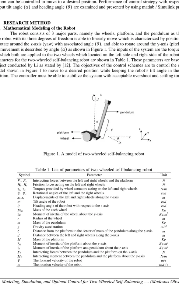
The robot consists of 3 major parts, namely the wheels, platform, and the pendulum as the mass. The robot with its three degrees of freedom is able to linearly move which is characterized by position x, able to rotate around the z-axis (yaw) with associated angle ( ), and able to rotate around the y-axis (pitch) where the movement is described by angle ( ) as shown in Figure 1. The inputs of the system are the torques and which both are applied to the two wheels which located on the left side and right side of the robot. List of parameters for the two-wheeled self-balancing robot are shown in Table 1. These parameters are based on the project conducted by Li as stated by [12]. The objectives of the control schemes are to control the system’s model shown in Figure 1 to move to a desired position while keeping the robot’s tilt angle in the upright position. The controller must be able to stabilize the system with acceptable overshoot and settling time.

Figure 1. A model of two-wheeled self-balancing robot

Table 1. List of parameters of two-wheeled self-balancing robot

Symbol Parameter Unit

Fl , Fr Interacting forces between the left and right wheels and the platform N

Hl , Hr Friction forces acting on the left and right wheels N Torques provided by wheel actuators acting on the left and right wheels N/m

Rotational angles of the left and the right wheels rad xl, xr Displacements of the left and right wheels along the x-axis m

Tilt angle of the robot rad

Heading angle of the robot with respect to the z-axis rad

MW Mass of the each wheel Kg

IW Moment of inertia of the wheel about the y-axis Kg.m2

r Radius of the wheel m

m Mass of the pendulum Kg

g Gravity acceleration m/s2

Distance from the platform to the center of mass of the pendulum along the z-axis m d Distance between the left and right wheels along the y-axis m

M Mass of the platform Kg

IM Moment of inertia of the platform about the y-axis Kg.m2

IP Moment of inertia of the platform and pendulum about the z-axis Kg.m2

FP Interacting forces between the pendulum and the platform on the x-axis N

MP Interacting moment between the pendulum and the platform about the y-axis N/m

V The forward velocity of the robot m/s

(3)

With assumption that there is no slip between the wheels and the ground, by applying Newton’s law for the linear and rotational motion based [13] and [14], balancing forces and moment acting on the left wheel results in the following equations of motion:

∑ ̈ ( ) (1)

∑ ̈ (2)

Similiarly, for the right wheel we have:

∑ ̈ ( ) (3)

∑ ̈ (4)

Balancing forces acting on the pendulum on the x-axis direction and moments between the pendulum and the platform about the y-axis results in:

̈ ̈ ̇ (5)

̈ (6)

̈ ̈ (7)

̈ (8)

Balancing the moments acting on the platform and pendulum about the z-axis gives:

̈ ( ) (9)

The relationship between the displacements of the wheel along the x-axis and the rotational angle of the wheel about the y-axis is:

(10)

On the other hand, the relationship between the heading angle ( ) of the robot about the z-axis and the displacement of the wheel along the x-axis is:

(11)

By subtracting (1) and (2) from (3) and (4) respectively then substituting it to (11) result in:

( ̈ ̈ ) ( ) (12) ( ̈ ̈) ( ) (13) ( ) ̈ ( ) ( ) (14) ̈ ( ( ) ) ( ) (15)

By adding (1) and (2) with (3) and (4) respectively then substituting it to (10), we have:

̈ ( ) (16)

(4)

Adding (16) and (17) we have:

( ) ̈ ( ) (18)

By substituting (18) to (5) and (6) we obtain:

̈ ( ( )) ̈ ̇ (19)

By substituting (7) to (8) result in:

( ) ̈ ̈ (20)

From the above derivation, we can obtain the dynamics equation of motion of the two-wheeled self-balancing robot as (15), (19), and (20). Assuming that the robot only around a small operating point, the dynamic model of the robot is then linearized around the point ̇ . Equation (19), and (20) then became:

̈ ( ( )) ̈ (21)

( ) ̈ ̈ (22)

By defining the following 5-dimensional vector of state variable:

[ ] [

̇ ̇]

(23)

Using (15), (21), and (22) the linearized two-wheeled self-balancing robot model can be expressed in the following state-space form:

[ ̇ ̈ ̇ ̇ ̈] [ ] [ ̇ ̇] [ ] * + (24) where: ( ( )) (( ( )) ( )) (25) (( ( )) ( )) (26) ( (( ( )) ( ))) (27) ( (( ( )) ( ))) (28) ( (( ( )) ( ))) (29)

(5)

( (( ( )) ( ))) (30) ( ( )) (31) ( ( )) (32)

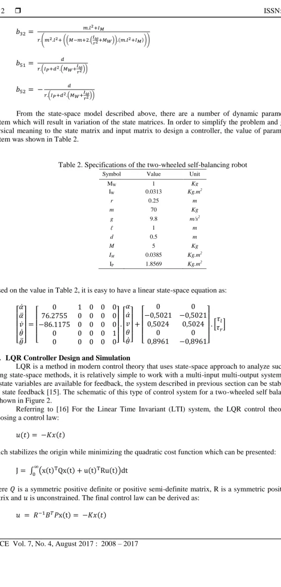
From the state-space model described above, there are a number of dynamic parameters in the system which will result in variation of the state matrices. In order to simplify the problem and give a clear physical meaning to the state matrix and input matrix to design a controller, the value of parameters of the system was shown in Table 2.

Table 2. Specifications of the two-wheeled self-balancing robot

Symbol Value Unit

MW 1 Kg IW 0.0313 Kg.m2 r 0.25 m m 70 Kg g 9.8 m/s2 1 m d 0.5 m M 5 Kg IM 0.0385 Kg.m2 IP 1.8569 Kg.m2

Based on the value in Table 2, it is easy to have a linear state-space equation as:

[ ̇ ̈ ̇ ̇ ̈] [ ] [ ̇ ̇] [ ] * + (33)

2.2. LQR Controller Design and Simulation

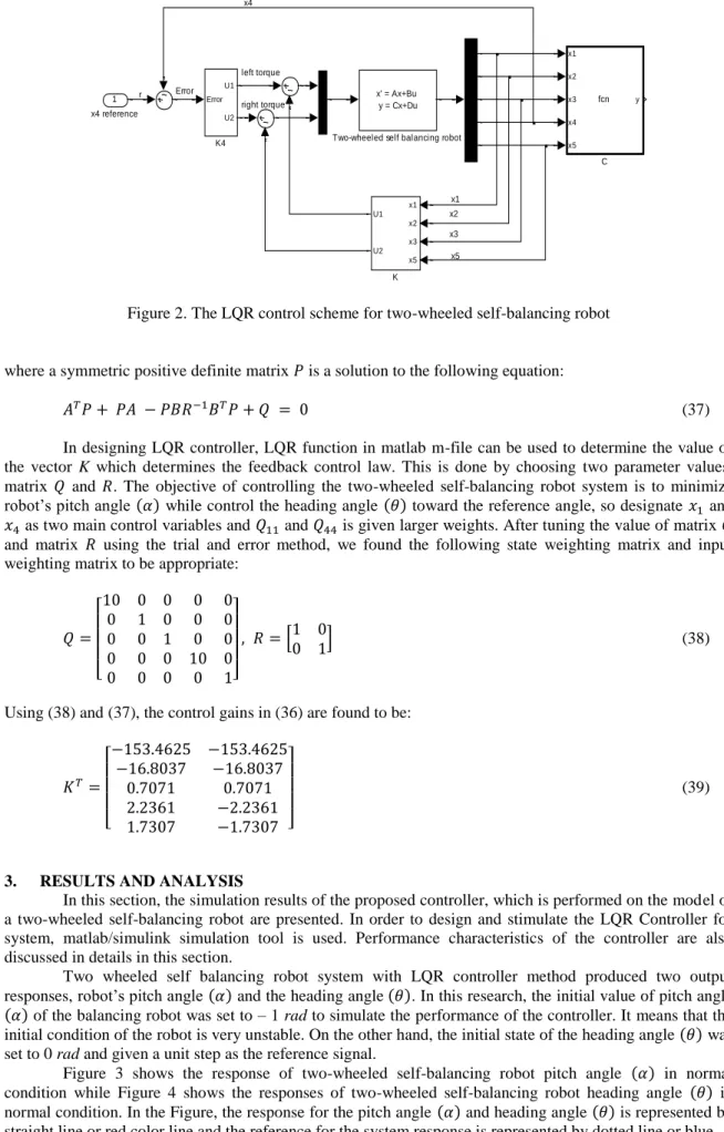
LQR is a method in modern control theory that uses state-space approach to analyze such a system. Using state-space methods, it is relatively simple to work with a multi-input multi-output system. Assuming all state variables are available for feedback, the system described in previous section can be stabilized using full state feedback [15]. The schematic of this type of control system for a two-wheeled self balancing robot is shown in Figure 2.

Referring to [16] For the Linear Time Invariant (LTI) system, the LQR control theory involves choosing a control law:

( ) ( ) (34)

which stabilizes the origin while minimizing the quadratic cost function which can be presented:

∫ ( ( ) ( ) ( ) ( )) (35)

where is a symmetric positive definite or positive semi-definite matrix, R is a symmetric positive definite matrix and is unconstrained. The final control law can be derived as:

(6)

Figure 2. The LQR control scheme for two-wheeled self-balancing robot

where a symmetric positive definite matrix is a solution to the following equation:

₍₃₇₎

In designing LQR controller, LQR function in matlab m-file can be used to determine the value of the vector K which determines the feedback control law. This is done by choosing two parameter values, matrix and . The objective of controlling the two-wheeled self-balancing robot system is to minimize robot’s pitch angle ( ) while control the heading angle ( ) toward the reference angle, so designate and

as two main control variables and and is given larger weights. After tuning the value of matrix and matrix using the trial and error method, we found the following state weighting matrix and input weighting matrix to be appropriate:

[ ] * + (38)

Using (38) and (37), the control gains in (36) are found to be:

[ ] (39)

3. RESULTS AND ANALYSIS

In this section, the simulation results of the proposed controller, which is performed on the model of a two-wheeled self-balancing robot are presented. In order to design and stimulate the LQR Controller for system, matlab/simulink simulation tool is used. Performance characteristics of the controller are also discussed in details in this section.

Two wheeled self balancing robot system with LQR controller method produced two output responses, robot’s pitch angle ( ) and the heading angle ( ). In this research, the initial value of pitch angle

( ) of the balancing robot was set to – 1 rad to simulate the performance of the controller. It means that the initial condition of the robot is very unstable. On the other hand, the initial state of the heading angle ( ) was set to 0 rad and given a unit step as the reference signal.

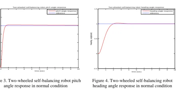
Figure 3 shows the response of two-wheeled self-balancing robot pitch angle ( ) in normal condition while Figure 4 shows the responses of two-wheeled self-balancing robot heading angle ( ) in normal condition. In the Figure, the response for the pitch angle ( ) and heading angle ( ) is represented by straight line or red color line and the reference for the system response is represented by dotted line or blue

Error r x1 x2 x3 x5 x4 left torque right torque x' = Ax+Bu y = Cx+Du

Two-wheeled self balancing robot Error U1 U2 K4 x1 x2 x3 x5 U1 U2 K x1 x2 x3 x4 x5 y fcn C 1 x4 reference

(7)

color line. From the figure, it can be seen that the LQR controller are capable to control the pitch angle and heading angle of the robot to the desired value. The settling time for the pitch angle to reach balance state in 2.23 sec while the steady-state error is 0.0086 rad. Meanwhile, the settling time for the heading angle to reach the steady-state value is 2.76 sec while the steady-state error is 0 rad. The control effort of the system’s response is as shown in Figure 5. The torques applied to the left and the right wheel show a slight difference. This is due to the desired value of the system’s heading angle = 1 rad and the system try to follow the reference signal.

Figure 3. Two-wheeled self-balancing robot pitch angle response in normal condition

Figure 4. Two-wheeled self-balancing robot heading angle response in normal condition

Figure 6 shows the response of two-wheeled self-balancing robot pitch angle ( ) with the pendulum’s mass being decreased to 40 Kg. From the figure it can be seen that the LQR controller are capable to control and balance the pitch angle despite the change in the pendulum’s mass. It show that the result has got similar pattern and not much different from the normal condition system. Almost no significant differences were apparent from controller’s performance in normal condition with decreased mass condition as shown by Figures 3 and Figure 6.

Figure 5. Control effort of two-wheeled self-balancing robot in normal condition

Figure 6. Two-wheeled self-balancing robot pitch angle response with decreased mass of the

pendulum = 40 Kg

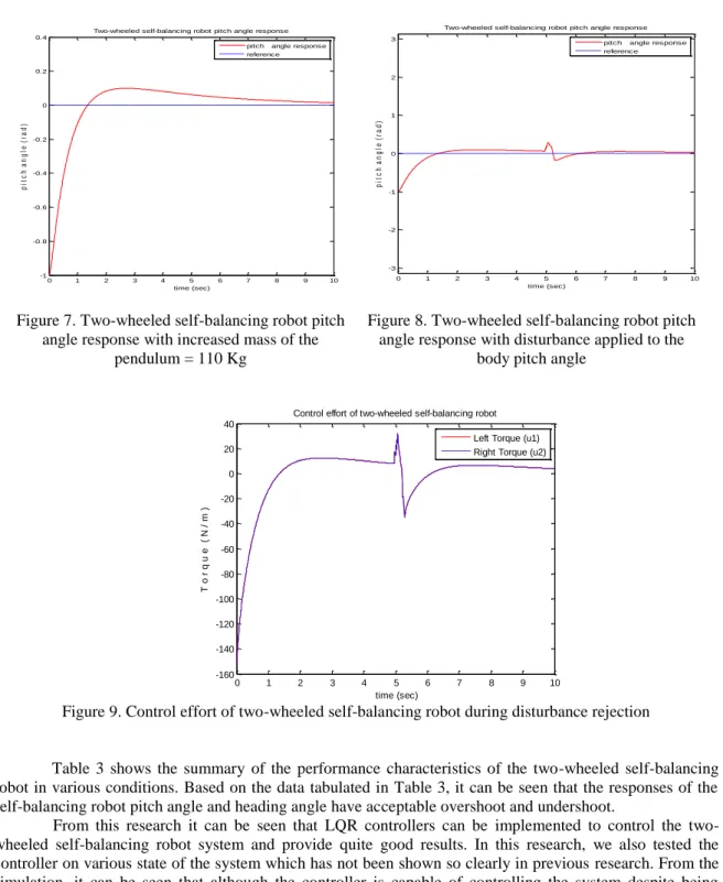
Meanwhile, Figure 7. shows the response of two-wheeled self-balancing robot pitch angle ( ) with the pendulum’s mass being increased to 110 Kg. From the figure it can be seen that the system’s response became a little bit quicker while changes in the steady-state error is relatively small and can be ignored. When the pendulum’s mass were being increased, there is a significance increase in system’s maximum

0 1 2 3 4 5 6 7 8 9 10 -1 -0.8 -0.6 -0.4 -0.2 0 0.2 0.4 time (sec) pi tc h an gl e (ra d)

Two-wheeled self-balancing robot pitch angle response pitch angle response reference 0 1 2 3 4 5 6 7 8 9 10 -0.5 0 0.5 1 1.5

Two-wheeled self-balancing robot heading angle response

He ad in g ag le (ra d) time (sec) 0 1 2 3 4 5 6 7 8 9 10 -1 -0.8 -0.6 -0.4 -0.2 0 0.2 0.4 time (sec) pi tc h an gl e (ra d)

Two-wheeled self-balancing robot pitch angle response pitch angle response reference 0 1 2 3 4 5 6 7 8 9 10 -0.5 0 0.5 1 1.5 time (sec) He ad in g a ng le (ra d)

Two-wheeled self-balancing robot heading angle response heading angle response reference 0 1 2 3 4 5 6 7 8 9 10 -160 -140 -120 -100 -80 -60 -40 -20 0 20 time (sec) T o rq u e ( N / m )

Control effort of two-wheeled self-balancing robot

Left Torque (u1) Right Torque (u2)

0 1 2 3 4 5 6 7 8 9 10 -1 -0.8 -0.6 -0.4 -0.2 0 0.2 0.4 time (sec) p i t c h a n g l e ( r a d )

Two-wheeled self-balancing robot pitch angle response pitch angle response reference 0 1 2 3 4 5 6 7 8 9 10 -0.5 0 0.5 1 1.5 time (sec) H e a d i n g a n g l e ( r a d )

Two-wheeled self-balancing robot heading angle response heading angle response reference

(8)

overshoot and steady-state error but overall, the performance of the controller was still acceptable because it can still maintain it’s upright position. The performance of the controller in Figure 7 gives the conclusion that the performance of LQR controllers is limited to a certain range of pendulum’s mass from the normal conditions. If the pendulum mass is increased to a certain point, it is possible that the controller will fail to control the system so that the robot will fall. Therefore, when designing LQR controllers it should also take into account the range of pendulum’s mass in which the system will operate most.

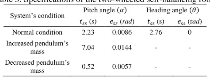
The disturbance rejection performance of the controller is shown in Figure 8. An impulse disturbance is applied at around 5 sec to the robot while it is stabilizing. It can be observed that the robot is able to reject this disturbance and regains its balance position in a short amount of time. A greater control effort is used by the robot to overcome the disturbance force as shown in Figure 9.

Figure 7. Two-wheeled self-balancing robot pitch angle response with increased mass of the

pendulum = 110 Kg

Figure 8. Two-wheeled self-balancing robot pitch angle response with disturbance applied to the

body pitch angle

Figure 9. Control effort of two-wheeled self-balancing robot during disturbance rejection

Table 3 shows the summary of the performance characteristics of the two-wheeled self-balancing robot in various conditions. Based on the data tabulated in Table 3, it can be seen that the responses of the self-balancing robot pitch angle and heading angle have acceptable overshoot and undershoot.

From this research it can be seen that LQR controllers can be implemented to control the two-wheeled self-balancing robot system and provide quite good results. In this research, we also tested the controller on various state of the system which has not been shown so clearly in previous research. From the simulation, it can be seen that although the controller is capable of controlling the system despite being subjected to a change in mass or disturbance to the body pitch angle, there is a tolerable limit of mass change

0 1 2 3 4 5 6 7 8 9 10 -1 -0.8 -0.6 -0.4 -0.2 0 0.2 0.4 time (sec) p i t c h a n g l e ( r a d )

Two-wheeled self-balancing robot heading angle response heading angle response reference 0 1 2 3 4 5 6 7 8 9 10 -3 -2 -1 0 1 2 3 time (sec) p i t c h a n g l e ( r a d )

Two-wheeled self-balancing robot heading angle response heading angle response reference 0 1 2 3 4 5 6 7 8 9 10 -160 -140 -120 -100 -80 -60 -40 -20 0 20 40 time (sec) T o r q u e ( N / m )

Control effort of two-wheeled self-balancing robot Left Torque (u1) Right Torque (u2)

(9)

or pitch angle change. Therefore, when designing the controller, the values of the system parameters should be considered sothat the controller can work well under ideal or non ideal conditions.

Table 3. Specifications of the two-wheeled self-balancing robot

System’s condition Pitch angle ( ) Heading angle ( ) (s) (rad) (s) (rad) Normal condition 2.23 0.0086 2.76 0 Increased pendulum’s mass 7.04 0.0144 - - Decreased pendulum’s mass 0.52 0.0057 - - 4. CONCLUSION

In this paper, the design and implementation of LQR controller for stabilizing a two-wheeled self-balancing robot is presented. The performance of LQR is simulated and analyzed with matlab/simulink program. Based on the results and the analysis, a conclusion has been made that the LQR controller are capable of controlling the two-wheeled self-balancing robot’s pitch angle and heading angle and yields acceptable and good results without falling. In normal condition the system can be engaged to balance itself and give transient response characteristics settling time = 2.23 sec and steady-state error = 0.0086 rad for tilt angle response and settling time = 2.76 sec and steady-state error = 0 rad for heading angle response. When the pendulum’s mass is being increased by 30 Kg, the system give transient response characteristics settling time = 7.04 sec and steady-state error = 0.0144 rad for tilt angle and when the pendulum’s mass is being decreased by 30 Kg the system give transient response characteristics settling time = 0.52 sec and steady-state error = 0.0057 rad for tilt angle. However, more experiment needs to be performed to evaluate the robustness of the system. Nonlinear controller is fully recommended for balancing the two-wheeled self-balancing robot as it will upgrade the robustness of the system.

REFERENCES

[1] A.N.K. Nasir, M.A. Ahmad, R.M.T. Raja Ismail, “The Control of a Highly Nonlinear Two-wheels Balancing Robot: A Comparative Assessment between LQR and PID-PID Control Schemes”, in International Journal of Mechanical, Aerospace, Industrial, Mechatronic, and Manufacturing Engineering, vol. 4, no. 10, pp. 942-947, October 2010.

[2] H. Liu, J. Xu, Y. Sun, “Adaptive Fuzzy Sliding Mode Stabilization Controller for Inverted Pendulums”, in Telecommunication, Computing, Electronics, and Control (TELKOMNIKA), vol. 11, no. 12, pp. 7243-7250, December 2013.

[3] T.Y. Chuan, L. Feng, Q. Qian, Y. Yang, “Stabilizing Planar Inverted Pendulum Systems Based on Fuzzy Nine-Point Controller”, in Telecommunication, Computing, Electronics, and Control (TELKOMNIKA), vol. 12, no. 1, pp. 422-432, January 2014.

[4] T.O.S Hanafy, M.K. Metwally, “Simplifications the Rule Base for Stabilization of Inverted Pendulum System”, in Telecommunication, Computing, Electronics, and Control (TELKOMNIKA), vol. 12, no. 7, pp. 5225-5234, July 2014.

[5] M. ul Hasan, K.M. Hasam, et al., “Design and Experimental Evaluation of a State Feedback Controller for Two Wheeled Balancing Robot”, 17th IEEE International Multi Topic Conference (INMIC), Karachi, 2014:366-371. [6] Jian Fang, “The LQR Controller Design of Two-wheeled Self-balancing Robot Based on the Particle Swarm

Optimization Algorithm”, in Mathematical Problems in Engineering, vol.2014, article id.729095, pp. 1- 6, June 2014.

[7] K. Prakash, K. Thomas, “Study of Controller for a Two Wheeled Self-balancing Robot”, International Conference on Next Generation Intelligent Systems (ICNGIS), Kottayam, 2016.

[8] H.S. Zad, A. Ulasyar, A. Zohaib, and S.S. Hussain, “Optimal Controller Design for Self-balancing Two-wheeled Robot System”, International Conference on Frontiers of Information Technology (FIT), Islamabad. 2016:11-16. [9] C. Sun, T. Lu, K. Yuan, “Balance Control of Two-wheeled Self-balancing Robot Based on Linear Quadratic

Regulator and Neural Network”, 4th International Conference on Intelligent Control and Information Processing (ICICIP), Beijing, 2013:862-867.

[10] M. Majczak, P. Wawrzyński, “Comparison of Two Efficient Control Strategies for Two-wheeled Balancing Robot”, 20th International Conference on Methods and Models in Automation and Robotics (MMAR), Miedzyzdroje, 2015:744-749.

[11] Mikael Arvidsson, Jonas Karlsson, “Design, Construction and Verification of a Self-balancing Vehicle”, Chalmers University of Technology, Department of Signals and Systems, Report number: EX050, 2012

(10)

[12] Zhijun Li, Chenguang Yang, Liping Fan, “Advanced Control of Wheeled Inverted Pendulum Systems”, London: Springer, 2013.

[13] David Morin, “Introduction to Classical Mechanincs with Problems and Solutions”, New York: Cambridge University Press, 2008.

[14] H. D. Young, R. A. Freedman, “University Physics with Modern Physics”, Twelfth Edition. San Fransisco: Pearson Adisson-Wesley, 2007.

[15] Katsuhiko Ogata, “Modern Control Engineering”, Third Edition, New Jersey: Prentice Hall, 1997. [16] R.C. Dorf, R.H. Bishop, “Modern Control System, Twelfth Edition, New Jersey: Prentice Hall, 2011.

BIOGRAPHIES OF AUTHORS

Modestus Oliver Asali was born in Pontianak, Indonesia, in 1994. He received his Bachelor’s degree with a concentration in control engineering from Department of Electrical, Tanjungpura University, Pontianak in 2017. He is interested in modern control engineering, and control of nonlinear dynamical system. He now lived in Pontianak and may be reached at [email protected]

Ferry Hadary is an Assistant Professor of Robotics, Control and Computation at Tanjungpura University (UNTAN), Pontianak, Indonesia. He earned his B.Eng. degree from Tanjungpura University, M. Eng. from Tokyo Institute of Technology, Japan, and Dr. Eng. from Kyushu Institute of Technology, Japan. He is currently teaching at Department of Electrical Engineering, Tanjungpura University. In his career as a researcher he received several research grants prestige of the Ministry of Research Technology and Higher Education of the Republic of Indonesia, Grants International Cooperation and the National Strategic (highest research grants in Indonesia). He is also a recipient of the National Work Featured Technology of the Ministry of Research and Technology of Indonesia in 2014. His interests are in control systems, robotics, new and renewable energy. He may be reached at [email protected]

Bomo Wibowo Sanjaya was born in Pontianak, Indonesia, in 1974. He received his Bachelor’s degree in control engineering from Department of Electrical, Tanjungpura University, Pontianak in 2008, his Master’s Degree in control engineering from Department of Electrical, Bandung Institute of Technology in 2013, and his Doctor’s Degree in control engineering from School of Electrical Engineering and Informatics, Bandung Institute of Technology in 2014. Now, he is a lecturer at Department of Electrical, Tanjungpura University. He current research interests are in fuzzy logic, neural networks, control of nonlinear dynamical systems. He may be reached at [email protected]