Benchmarking Image Processing Algorithms for Unmanned Aerial System-Assisted Crack Detection in Concrete Structures

(1)

DigitalCommons@University of Nebraska - Lincoln

Architectural Engineering -- Faculty Publications

Architectural Engineering and Construction,

_{Durham School of}

2019

Benchmarking Image Processing Algorithms for Unmanned Aerial

System-Assisted Crack Detection in Concrete Structures

Sattar Dorafshan

Robert J. Thomas

Marc Maguire

Follow this and additional works at: https://digitalcommons.unl.edu/archengfacpub

Part of the Architectural Engineering Commons, Construction Engineering Commons, Environmental Design Commons, and the Other Engineering Commons

This Article is brought to you for free and open access by the Architectural Engineering and Construction, Durham School of at DigitalCommons@University of Nebraska - Lincoln. It has been accepted for inclusion in Architectural Engineering -- Faculty Publications by an authorized administrator of DigitalCommons@University of Nebraska - Lincoln.

(2)

infrastructures

Article

Benchmarking Image Processing Algorithms for

Unmanned Aerial System-Assisted Crack Detection

in Concrete Structures

Sattar Dorafshan1,_{*, Robert J. Thomas}2 _{and Marc Maguire}3

1 _O_ffi_{ce of Infrastructure Research and Development, Turner-Fairbank Highway Research Center,} Federal Highway Administration, Sterling, VA 22101, USA

2 _{Department of Civil and Environmental Engineering, Clarkson University, Potsdam, NY 13699-5710, USA;} [email protected]

3 _{Department of Civil and Environmental Engineering, Utah State University, Logan, UT 84322-4110, USA;} [email protected]

* Correspondence: [email protected]

Received: 24 March 2019; Accepted: 29 April 2019; Published: 30 April 2019

Abstract:This paper summarizes the results of traditional image processing algorithms for detection of defects in concrete using images taken by Unmanned Aerial Systems (UASs). Such algorithms are useful for improving the accuracy of crack detection during autonomous inspection of bridges and other structures, and they have yet to be compared and evaluated on a dataset of concrete images taken by UAS. The authors created a generic image processing algorithm for crack detection, which included the major steps of filter design, edge detection, image enhancement, and segmentation, designed to uniformly compare different edge detectors. Edge detection was carried out by six filters in the spatial (Roberts, Prewitt, Sobel, and Laplacian of Gaussian) and frequency (Butterworth and Gaussian) domains. These algorithms were applied to fifty images each of defected and sound concrete. Performances of the six filters were compared in terms of accuracy, precision, minimum detectable crack width, computational time, and noise-to-signal ratio. In general, frequency domain techniques were slower than spatial domain methods because of the computational intensity of the Fourier and inverse Fourier transformations used to move between spatial and frequency domains. Frequency domain methods also produced noisier images than spatial domain methods. Crack detection in the spatial domain using the Laplacian of Gaussian filter proved to be the fastest, most accurate, and most precise method, and it resulted in the finest detectable crack width. The Laplacian of Gaussian filter in spatial domain is recommended for future applications of real-time crack detection using UAS.

Keywords: structural condition assessment; concrete structures; unmanned aerial systems; crack detection; image processing; noncontact methods

1. Introduction

The United States is home to more than 600,000 bridges, more than one-third of which include a concrete superstructure or wear surface [1]. These bridges require a variety of periodic inspections in accordance with federal regulations. The most common inspection type is routine inspection, wherein the inspector scans the bridge deck to identify surface degradation or surface cracking. Such inspections are costly, time-consuming, and labor-intensive [2,3]. Autonomous inspection could be a cost-effective solution to these problems if the accuracy of human inspection can be matched [3–9]. Image-based inspection of infrastructure for concrete delamination [10–13], cracks [14–17], and spalls [18,19] using unmanned aerial systems (UASs) have been proven effective based on previous literature [20].

(3)

Image-based autonomous inspections still require human inspectors to review images. The number of images collected depends on a number of factors, but it is commonly in the several thousands. For instance, SDNET2018 [21], with more than 56,000 labeled images of concrete structures, covers three small lab-made bridge decks, walls of a building, and several paved sidewalks, which are significantly smaller than common inspected infrastructures in practice. Manual identification of flaws in such large image sets is time consuming and prone to inaccuracy because of inspector fatigue or human error [22–26]. Image processing algorithms can improve the accuracy and efficiency of autonomous inspections by either (a) enhancing images to improve ease of human detection of defects or (b) autonomously identifying defects. Additionally, edge detectors are used in combination with more contemporary techniques such as deep learning convolutional neural networks for UAS applications [27], reducing false positive cases by 20 times compared to sole use of edge detectors [28].

Cracks in a two-dimensional (2D) image are classified as edges, and, thus, existing edge detection algorithms are likely candidates for crack identification. 2D images are represented mathematically by matrices (one matrix, in the case of greyscale images, or three matrices in the case of red/green/blue color images). An ideal edge is defined as a discontinuity in the greyscale intensity field. Crack detection algorithms can emphasize edges by applying filters in either the spatial or frequency domain. Even though use of edge detectors for crack detection goes back to the early 2000s [29], these methods have been used in the past and are still being used in recent studies because of their simplicity and pixel-based detection of cracks [15,28,30–42]. Even in emerging applications of supervised machine learning methods, edge detectors are still considered in practice since they do not require expensive annotated training datasets. Using edge detectors for crack detection is computationally fast, making it an appealing option for real-time crack detection during UAS inspections; they have been implemented in ground-based robotic inspections in the past [4,18,38]. Edge detectors can have different sizes, shapes, and values. There are limited guidelines for researchers and practitioners in choosing a proper edge detector for their applications, especially for UAS collected data.

Save two noteworthy exceptions, most research focuses on developing new methods for crack detection rather than comparing the performance of existing methods. Abdel-Qader et al. [29] compared the performance of the fast Haar transform, Fourier transform, Sobel filter, and Canny filter for crack detection in 25 images of defected concrete and 25 images of sound concrete. The fast Haar transform was the most accurate method, with an overall accuracy of 86%, followed by the Canny filter (76%), Sobel filter (68%), and the Fourier transform (64%). Processing time was not considered, and no actual definition of accuracy was presented. Mohan and Poobal [43] reviewed a number of edge detection techniques for visual, thermal, and ultrasonic images, but the information presented was from several studies that considered vastly different data sets, and so the results were not directly comparable. This paper presents the results of a direct comparison of four common edge detection methods in the spatial domain (Roberts, Prewitt, Sobel, and Laplacian of Gaussian) and two in the frequency domain (Butterworth and Gaussian) by applying them to a dataset of 50 sound and 50 defected images of concrete collected from UAS. The goal of this study is to determine the most efficient edge detectors to use in aiding UAS condition assessments of concrete structures when all the other parameters are kept the same. Prior to implementation, as an emerging technology in bridge inspections, UAS need a rigorous investigation as part of a process model to determine whether they can be used in lieu of hands-on inspections. While this is not a part of this study, such an approach would involve investigating the reliability and effectiveness of UAS inspections through a generic decision making tool that includes a multivariable analysis of the inspection accuracy, cost, time, and hazard.

2. Analytical Program

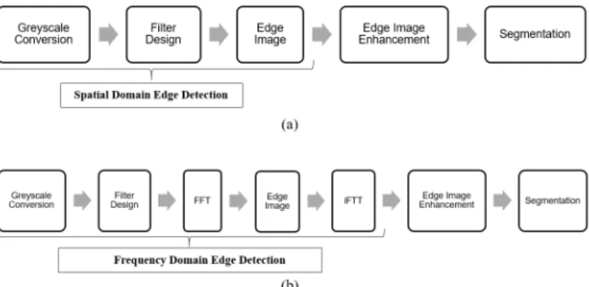
Figure1shows a generic image analysis algorithm developed for this study. The generic algorithm included three main steps: Edge detection, edge image enhancement, and segmentation. Edge detection in the spatial domain involved greyscale conversion and application of a filter. Edge detection in the frequency domain required additional steps to transform the image from the spatial domain to the

(4)

Infrastructures2019,4, 19 3 of 16

frequency domain before application of the filter. The inverse operation to transform the filtered image back to the spatial domain was also an additional step. This section includes the particulars of each step in the generic image processing algorithm.

Infrastructures 2019, 4, x FOR PEER REVIEW 3 of 16 Edge detection in the spatial domain involved greyscale conversion and application of a filter. Edge detection in the frequency domain required additional steps to transform the image from the spatial domain to the frequency domain before application of the filter. The inverse operation to transform the filtered image back to the spatial domain was also an additional step. This section includes the particulars of each step in the generic image processing algorithm.

Figure 1. The steps in the proposed crack detection algorithm. (a) The spatial domain and (b) the frequency domain.

2.1. Greyscale Conversion

Edge detection algorithms perform best with greyscale images [44], so the first step in the image analysis procedure was greyscale conversion of color images. The original color image comprised a matrix of pixels, each with a defined red, green, and blue intensity. Greyscale conversion followed Equation 1, where I(x, y) is the grayscale intensity of pixel (x, y), and R(x, y), G(x, y), and B(x, y)

are the red, green, and blue pixel intensities of the same, respectively.

𝐼(𝑥, 𝑦) = 0.2989𝑅(𝑥, 𝑦) + 0.5870𝐺(𝑥, 𝑦) + 0.1140𝐵(𝑥, 𝑦). (1)

2.2. Edge Detection in the Spatial Domain

In general, edge detection in images requires filtering by one of several common methods, which are discussed in detail below. Filters are applied as a small matrix of values (called a kernel) through a mathematical operation known as convolution. In general form, the convoluted image 𝐎 is the sum of the element-by-element products of the image intensity matrix 𝐈and the kernel 𝐊 in every position in which 𝐊 fits fully inside 𝐈. Equation 2 describes this in plainer terms for image size

M × N and kernel size m × n.

𝑂(𝑖, 𝑗) = ∑ ∑ℓ 𝐼(𝑖 + 𝑘 − 1, 𝑗 + ℓ − 1)𝐾(𝑘, ℓ), (2)

The convoluted image 𝐎 will be of size (M − m + 1) × (N − n + 1). The kernel typically includes both x and y components; the convoluted images E and E obtained from the x and

y components of the filter emphasize vertical and horizontal edges, respectively. The final edge image E is the square root of the sum of the squared component images, i.e.,

𝑂(𝑖, 𝑗) = ∑ ∑ℓ 𝐼(𝑖 + 𝑘 − 1, 𝑗 + ℓ − 1)𝐾(𝑘, ℓ). (3)

Common edge detecting filters in the spatial domain include Roberts, Prewitt, and Sobel. Equations 4–6 give the x and y kernels for the Roberts (R and R), Prewitt (P and P), and Sobel (S and S) filters. These filters compute the gradient between neighboring pixels in the x and y

directions and intensify areas of high gradient (i.e., edges). Filters are constructed such that the Figure 1. The steps in the proposed crack detection algorithm. (a) The spatial domain and (b) the frequency domain.

2.1. Greyscale Conversion

Edge detection algorithms perform best with greyscale images [44], so the first step in the image analysis procedure was greyscale conversion of color images. The original color image comprised a matrix of pixels, each with a defined red, green, and blue intensity. Greyscale conversion followed Equation (1), where I(x, y)is the grayscale intensity of pixel(x, y), and R(x, y), G(x, y), and B(x, y)are the red, green, and blue pixel intensities of the same, respectively.

I(x,y) =0.2989R(x,y) +0.5870G(x,y) +0.1140B(x,y). (1) 2.2. Edge Detection in the Spatial Domain

In general, edge detection in images requires filtering by one of several common methods, which are discussed in detail below. Filters are applied as a small matrix of values (called a kernel) through a mathematical operation known as convolution. In general form, the convoluted imageOis the sum of the element-by-element products of the image intensity matrixIand the kernelKin every position in whichKfits fully insideI. Equation (2) describes this in plainer terms for image size M×_{N and kernel} size m×_n.

O(i,j) =Xm

k=1

Xn

`=1I(i+k−1,j+`−1)K(k,`), (2) The convoluted imageOwill be of size(M−_m₊₁₎×₍_N−_n₊₁₎_{. The kernel typically includes} both x and y components; the convoluted images Exand Eyobtained from the x and y components of the filter emphasize vertical and horizontal edges, respectively. The final edge image E is the square root of the sum of the squared component images, i.e.,

O(i,j) =Xm

k=1

Xn

`=1I(i+k−1,j+`−1)K(k,`). (3) Common edge detecting filters in the spatial domain include Roberts, Prewitt, and Sobel. Equations (4)–(6) give the x and y kernels for the Roberts (Rxand Ry), Prewitt (Pxand Py), and Sobel (Sx and Sy) filters. These filters compute the gradient between neighboring pixels in the x and y directions and intensify areas of high gradient (i.e., edges). Filters are constructed such that the components are of opposite sign and the sum of all components is zero. The Roberts filter (Equation (4)) is a compact kernel, which could lead to very fast processing times. The Prewitt (Equation (5)) and Sobel (Equation (6)) filters use larger 3×_{3 kernels and are therefore more powerful but require}

(5)

extended computation times. The Prewitt is a first-order filter (the largest magnitude component is one); the second-order Sobel filter will likely produce an image with more intensified edges.

Rx= " 1 0 0 −₁ # , Ry= " 0 1 −₁ ₀ # , (4) OPx=           −₁ ₀ ₁ −₁ ₀ ₁ −₁ ₀ ₁           ,Py=           1 1 1 0 0 0 −₁ −₁ −₁           , (5) Sx=           −₁ ₀ ₁ −₂ ₀ ₂ −₁ ₀ ₁           ,Sy=           1 2 1 0 0 0 −₁ −₂ −₁           , (6)

Another popular edge detection method in the spatial domain is the Laplacian of Gaussian (LoG) function. When applied to an image with intensities I(x, y), the Laplacian operator∇2₌ ∂2I

∂x2 + ∂ 2_I ∂y2 emphasizes both edges and noise or artifact. The influence of noise can be reduced by first applying the Gaussian smoothing filter given by Equation (7), where x and y are the spatial coordinates within the Gaussian kernel andσis the standard deviation

G(x,y) = √1 2πσ2exp −x 2₊_y2 2σ2 ! . (7)

Equation (8) gives the Laplacian of the Gaussian, which can be pre-allocated for a given filter size m×_{n and standard deviation}σ.

LoG=∇2₍_G₍_x_,_y_{)) =} x 2₊_y2₋₂_σ2 4σ4 exp − x2+y2 2σ2 ! . (8)

Iterative optimization of the parameters m, n, andσis possible on an image-by-image basis, but it is convenient to predefine both the size and standard deviation. For the purposes of this study, the LoG kernel was defined as a square matrix with size equal to 0.5% of the maximum image dimension, and the standard deviation was defined as one-fourth the maximum image dimension. At first glance, it would appear that the larger 13×_{13 LoG filter would be more computationally intensive than the} smaller Roberts, Prewitt, and Sobel filters discussed previously. However, the LoG filter does not include x and y component kernels. Thus, only one convolution operation (Equation (2)) was required, and there was no need for the component transformation (Equation (3)).

2.3. Edge Detection in the Frequency Domain

Edge detection in the frequency domain requires transformation from the spatial domain to the frequency domain. This is quickly accomplished using the fast Fourier transform (FFT), which transforms the greyscale image intensities I(x, y)into the frequency components F(u, v). Unlike in the spatial domain, where the filter kernel is of arbitrary size, the filter kernel in the frequency domain is the same size as the image. The edge image E(u, v)in the frequency domain is the element-by-element product of the filter kernel K(u, v)and the frequency domain image F(u, v), i.e.,

E(u,v) =K(u,v)_F₍_u_,_v₎_, ₍₉₎

where _{denotes element-wise multiplication. Inverse fast Fourier transformation (iFFT) of the} frequency domain edge image E(u, v)gives the edge image in the spatial domain E(x, y).

The two most common frequency domain edge detection filters include Butterworth [45] and Gaussian [45–47] high pass filters. High pass filters attenuate frequencies above some defined cutoff frequency D0. Equation (10) gives the general form of the nth-order Butterworth filter kernel KB(u, v),

(6)

where D(u, v)is the distance between the pixel(u, v)and the origin of the frequency (the center of the M×_{N image), as defined by Equation (11).}

KB(u,v) =1− 1 1+ _D(u ,v) D0 2n , (10) D(u,v) = s u− _M 2 +1 2 + v− _N 2 +1 2 . (11)

Similarly, Equation (12) gives the general form of the Gaussian high pass filter kernel KG(u, v), where D(u,v) is again the distance between the pixel(u, v)and the frequency origin, andσis the assumed standard deviation of the frequency distribution.

KG(u,v) =1−e

−_D2_(u_,_v)

2σ2 _. ₍₁₂₎

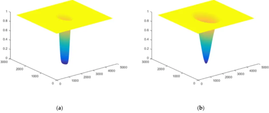
For the purposes of this study, a fourth order (n=4)Butterworth filter was constructed with cutoff frequency D0=M/10 The Guassian filter was constructed with standard deviationσ=M/10 Figure2 presents a graphical representation of the Butterworth and Gaussian filters.

Infrastructures 2019, 4, x FOR PEER REVIEW 5 of 16

𝐾 (𝑢, 𝑣) = 1 − _{( , )} , ₍₁₀₎

𝐷(𝑢, 𝑣) = 𝑢 − + 1 + 𝑣 − + 1 . (11) Similarly, Equation 12 gives the general form of the Gaussian high pass filter kernel K (u, v), where D(u,v) is again the distance between the pixel (u, v) and the frequency origin, and σ is the assumed standard deviation of the frequency distribution.

𝐾 (𝑢, 𝑣) = 1 − 𝑒 ( , ) . (12) For the purposes of this study, a fourth order (n = 4)Butterworth filter was constructed with cutoff frequency D0 = M/10 The Guassian filter was constructed with standard deviation σ = M/10 Figure 2 presents a graphical representation of the Butterworth and Gaussian filters.

(a) (b)

Figure 2. (a) Butterworth (n = 4, D = 259) and (b) Gaussian (σ = 259) filters for edge detection in the frequency domain.

2.4. Edge Image Enhancement

Edge images E(x, y) resulting from spatial or frequency domain edge detection filters contain a range of pixel intensities that require scaling. The scaling function given by Equation 13 converts edge image pixel intensities E(x, y) to linearly scaled edge image pixel intensities E (x, y) such that 0

I (x, y) 1.

𝐸 (𝑥, 𝑦) = 𝐸(𝑥, 𝑦) − 𝑚𝑖𝑛(𝐸) _{( )} _{( )}. (13) The scaled edge image E (x, y) requires contrast adjustment to improve edge clarity. Equation 14 transforms the scaled edge image E (x, y) into the enhanced edge image E (x, y), where μ and σ are the mean and standard deviation of the scaled edge image pixel intensities, respectively.

𝐸 (𝑥, 𝑦) = 𝐸 (𝑥, 𝑦) − 𝑚𝑖𝑛(𝐸 ) ₍ ₎ ₍ ₎ + 𝜇 . (14)

2.5. Segmentation

Segmentation was the final step in the proposed image analysis algorithm. This process converts the edge image to the binary image, in which pixels belonging to a crack take an intensity value of one, and the remaining pixels take an intensity value of zero. Selection of an appropriate threshold

Figure 2.(a) Butterworth (n=4, D0=259 ) and (b) Gaussian (σ=259)filters for edge detection in the frequency domain.

2.4. Edge Image Enhancement

Edge images E(x, y)resulting from spatial or frequency domain edge detection filters contain a range of pixel intensities that require scaling. The scaling function given by Equation (13) converts edge image pixel intensities E(x, y)to linearly scaled edge image pixel intensities Esc(x, y)such that 0≤_I_sc₍_{x, y}₎≤_1. Esc(x,y) = [E(x,y)−min(E)] " 1 max(E)−_min(E) # . (13)

The scaled edge image Esc(x, y)requires contrast adjustment to improve edge clarity. Equation (14) transforms the scaled edge image Esc(x, y)into the enhanced edge image Ee(x, y), whereµEscandσEsc are the mean and standard deviation of the scaled edge image pixel intensities, respectively.

Ee(x,y) = [Esc(x,y)−min(Esc)] " 2σEsc max(Esc)−min(Esc) # +µ_E_sc . (14) 2.5. Segmentation

Segmentation was the final step in the proposed image analysis algorithm. This process converts the edge image to the binary image, in which pixels belonging to a crack take an intensity value of one, and the remaining pixels take an intensity value of zero. Selection of an appropriate threshold

(7)

intensity—above which a pixel is classified as a crack and below which it is not—is critical. If the threshold intensity is too high, cracks go undetected. If it is too low, the image becomes noisy, and it is difficult to differentiate cracks from noise. This work considered two threshold operations for segmentation: pixel threshold and area threshold.

The pixel threshold operation follows Equation (15), where B1(x, y)is the first-level binary image, and T1is the pixel threshold value.

B1(x,y) = (

0, Ee(x,y)<T1 1, Ee(x,y)≥T1

. (15)

T1can be selected using Otsu’s method [47] or other intuitive/adaptive approaches [31]. In this study, T1 was selected based on the statistical properties of pixel intensities in the enhanced edge image Ee(x, y). Equation (16) defines T1, whereµEeandσEeare the mean and standard deviation of the enhanced edge image pixel intensities.

T1= µEe+3σEe. (16)

Similarly, the area threshold operation follows Equation (17), whereB2(x,y)is the second-level binary image andT2is the area threshold value.

B2(x,y) = (

0, B1(x,y)<T2

1, B1(x,y)≥T2 . (17)

Equation (18) defines T2according to the area of each connected component Acc, whereσAccis the standard deviation of the areas of connected components in B1.

T2=σAcc . (18)

The area of connected components Accis determined according to eight-neighbor connectivity, which considers pixel connectivity in the vertical, horizontal, or diagonal directions, such that pixel(x, y) is connected to all pixels(x±_{1, y}±₁₎_{. A}_cc_{could alternatively be defined according to four-neighbor} connectivity, which is a stricter definition that only considers connectivity in the vertical and horizontal directions, such that pixel(x, y)is connected to pixels(x±_{1, y})and(x, y±₁). For the purposes of this research, the more relaxed eight-neighbor definition of connectivity was adopted.

The second-level binary image B2is the final product of the proposed crack detection algorithm. 3. Experimental Program

In order to test the crack detection algorithm discussed above, the researchers gathered 50 images of sound concrete and 50 images of cracked concrete from several previously tested concrete panels at the Systems, Materials, and Structural Health Laboratory (SMASH Lab) at Utah State University. Images were taken with a 12 MP digital camera with focal length of 35 mm. The distance between the lens and the surface was approximately 0.3 m given the ability of the UAS to hold its position. The surface illumination, as verified by a Digi-Sense data logging light meter with NIST traceable calibration, was 1500–5000 lx. The image resolution was 2592×_{4608 px, and the approximate field} size was 1.0×_{1.2 m. RGB images were saved in JPEG format. Image processing was performed} in MATLAB on a 64-bit operating system with 32 GB memory and 3.40 GHz processor. Figure3

shows representative images of defected and sound concrete. Images were processed in six iterations, corresponding to the four spatial domain edge detectors and two frequency domain edge detectors.

(8)

(a) (b)

Figure 3.Representative images of (a) cracked concrete and (b) sound concrete.

Following image processing, an inspector reviewed the second-level binary images resulting from each of the six iterations in random order and classified each image as cracked or sound. The inspector reviewed only the second-level binary images; they did not review the original images or images from intermediate steps in the crack detection algorithm. The same inspector reviewed all of the images. The team then compared the results of each inspection to the ground truth, i.e., the known classification of each image as defected or sound based on physical inspection of the concrete surface aided by a crack microscope. The team then recorded the number of true positives (TPs), true negatives (TNs), false positives (FPs), and false negatives (FNs) for each iteration of the crack detection algorithm. A TP was a defected image in which the inspector accurately identified the defect. A TN was a sound image that the inspector accurately identified as sound. An FP was a sound image within which the inspector inaccurately identified a defect. An FN was a defected image that the inspector inaccurately identified as sound. A hit required the inspector to identify at least half of the actual crack length in a defected image. FP occurred when the inspector identified a crack in the noise or artifact of the second-level binary image. The performances of each approach of crack detection were evaluated in terms of accuracy, precision, processing time, and missed crack width (MCW). Accuracy, Ac., and precision, Pr., were calculated according to the following equations:

𝐴𝑐. = 𝑇𝑃+𝑇𝑁

𝑇𝑃+𝐹𝑃+𝑇𝑁+𝐹𝑁 ; (19)

𝑃𝑟 = 𝑇𝑃

𝑇𝑃+𝐹𝑃 . (20)

To obtain the processing time, each method of crack detection was run ten times on the same

desktop and the same dataset, and the mean of the processing times was reported as each method’s

processing time. In order to find MCW, the missed cracks by each crack detection method were identified and then measured using a crack microscope with 0.02 mm resolution. The algorithms were also compared in terms of the pixel intensity range in the enhanced edge images and the noise-to-signal

ratio (N/S). A wider range of pixel intensities suggested a sharper contrast between defects and sound

regions. N/S described the level of noise or artifact in the image and was defined as the ratio of lit pixels

(ones) to the total number of pixels in the second-level binary image B2. N/S was only computed for

the sound dataset because any lit pixels were known to be noise and not defects. A lower N/S was

greatly preferred because defects became more difficult to resolve when the image was noisy.

4. Results

Table 1 summarizes the results of the six iterations of the proposed crack detection algorithm. The TP rate (TPR), TN rate (TNR), FP rate (FPR), and FN rate (FNR) in the table are the percentages of TP, TN, FP, and FN reports. Note that the reported metrics in this paper were inclusive to the defined parameters in experimental and analytical procedures, and the authors were not suggesting that one could get similar results in practice with less-controlled situations.

Figure 3.Representative images of (a) cracked concrete and (b) sound concrete.

Following image processing, an inspector reviewed the second-level binary images resulting from each of the six iterations in random order and classified each image as cracked or sound. The inspector reviewed only the second-level binary images; they did not review the original images or images from intermediate steps in the crack detection algorithm. The same inspector reviewed all of the images. The team then compared the results of each inspection to the ground truth, i.e., the known classification of each image as defected or sound based on physical inspection of the concrete surface aided by a crack microscope. The team then recorded the number of true positives (TPs), true negatives (TNs), false positives (FPs), and false negatives (FNs) for each iteration of the crack detection algorithm. A TP was a defected image in which the inspector accurately identified the defect. A TN was a sound image that the inspector accurately identified as sound. An FP was a sound image within which the inspector inaccurately identified a defect. An FN was a defected image that the inspector inaccurately identified as sound. A hit required the inspector to identify at least half of the actual crack length in a defected image. FP occurred when the inspector identified a crack in the noise or artifact of the second-level binary image. The performances of each approach of crack detection were evaluated in terms of accuracy, precision, processing time, and missed crack width (MCW). Accuracy, Ac., and precision, Pr., were calculated according to the following equations:

Ac.= TP+TN

TP+FP+TN+FN ; (19)

Pr= TP

TP+FP (20)

To obtain the processing time, each method of crack detection was run ten times on the same desktop and the same dataset, and the mean of the processing times was reported as each method’s processing time. In order to find MCW, the missed cracks by each crack detection method were identified and then measured using a crack microscope with 0.02 mm resolution. The algorithms were also compared in terms of the pixel intensity range in the enhanced edge images and the noise-to-signal ratio (N/S). A wider range of pixel intensities suggested a sharper contrast between defects and sound regions. N/S described the level of noise or artifact in the image and was defined as the ratio of lit pixels (ones) to the total number of pixels in the second-level binary image B2. N/S was only computed for the sound dataset because any lit pixels were known to be noise and not defects. A lower N/S was greatly preferred because defects became more difficult to resolve when the image was noisy. 4. Results

Table1summarizes the results of the six iterations of the proposed crack detection algorithm. The TP rate (TPR), TN rate (TNR), FP rate (FPR), and FN rate (FNR) in the table are the percentages of TP, TN, FP, and FN reports. Note that the reported metrics in this paper were inclusive to the defined

(9)

parameters in experimental and analytical procedures, and the authors were not suggesting that one could get similar results in practice with less-controlled situations.

Table 1.Performance of different edge detectors in the proposed crack detection algorithm.

Domain Edge Detector TPR

1 (%) TNR2 (%) FPR3 (%) FNR4 (%) Ac.5 (%) Pr.6 (%) MCW7 (mm) Time (s) Spatial Roberts 64 90 10 36 77 86 0.4 1.67 Spatial Prewitt 82 82 18 18 82 82 0.2 1.4 Spatial Sobel 86 84 16 14 85 84 0.2 1.4

Spatial Laplacian of Gaussian (LoG) 98 86 14 2 92 88 0.1 1.18

Frequency Butterworth 80 86 14 20 83 85 0.2 1.81

Frequency Gaussian 80 88 12 20 84 87 0.2 1.92

1_{Ture Positive Rate,}2_{Ture Negative Rate,}3_{False Positive Rate,}4_{False Negative Rate,}5_Accuracy,6_Precision,

and7_{Missed Crack Width.}

In order to gain perspective about the numbers in this table, the accuracy of visual inspections should be determined. Washer et al. investigated the quality of element-level bridge inspection data. A required accuracy was arbitrary in visual inspections because the achieved accuracy was tied to the inspection process itself and was unaffected by the requirement [48]. Different inspectors responded very differently when inspecting the same structure or defect. The coefficients of variation of a rated bridge deck by different inspectors in visual inspections were between 57% and 96%. Detection of concrete deck cracks can be considered a “typical” decision in bridge inspections, and considering a normal distribution for all the calls, it is acceptable to have 67.5% of correct calls, i.e.,±_{one standard} deviation, [23,26,48]. This meant each of the edge detectors, except for Roberts, had surpassed the acceptable accuracy of the visual inspections. A bridge inspector reviewed the images in this study and was able to label all of the images correctly into sound and defected images (100% accuracy). Unlike the edge detectors, the inspector did not localize the pixels associated with cracks in the images, since it was very time-consuming, to provide a pixel-segmented ground truth [28]. This gave the edge detectors an advantage over human inspectors.

4.1. Spatial Domain, Roberts Filter

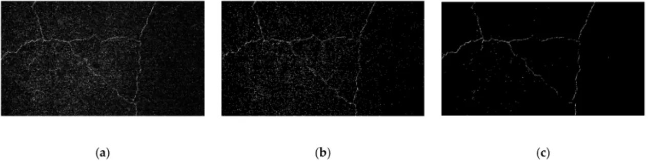
Crack detection in the spatial domain using the Roberts filter resulted in the lowest number of TPs (32), but it also resulted in the lowest FP (5). Thus, while the Roberts filter was the least accurate (77%), its precision (86%) was among the highest. The minimum detectable crack width was 0.4 mm and was the largest of the six edge detectors evaluated. The processing time (1.67 s per image) was near the median of the six methods evaluated. Figure4shows representative enhanced edge, first-level binary, and second-level binary images from spatial domain edge detection of an image from the defected set (Figure3a) using the Roberts filter.

Infrastructures 2019, 4, 19 8 of 16

In order to gain perspective about the numbers in this table, the accuracy of visual inspections should be determined. Washer et al. investigated the quality of element-level bridge inspection data. A required accuracy was arbitrary in visual inspections because the achieved accuracy was tied to the inspection process itself and was unaffected by the requirement [48]. Different inspectors responded very differently when inspecting the same structure or defect. The coefficients of variation of a rated bridge deck by different inspectors in visual inspections were between 57% and 96%. Detection of concrete deck cracks can be considered a “typical” decision in bridge inspections, and considering a normal distribution for all the calls, it is acceptable to have 67.5% of correct calls, i.e., ± one standard deviation, [23,26,48]. This meant each of the edge detectors, except for Roberts, had surpassed the acceptable accuracy of the visual inspections. A bridge inspector reviewed the images in this study and was able to label all of the images correctly into sound and defected images (100% accuracy). Unlike the edge detectors, the inspector did not localize the pixels associated with cracks in the images, since it was very time-consuming, to provide a pixel-segmented ground truth [28]. This gave the edge detectors an advantage over human inspectors.

Table 1. Performance of different edge detectors in the proposed crack detection algorithm.

Domain Edge Detector TPR1 (%) TNR2 (%) FPR3 (%) FNR4 (%) Ac.5 (%) Pr.6 (%) MCW7 (mm) Time (s) Spatial Roberts 64 90 10 36 77 86 0.4 1.67 Spatial Prewitt 82 82 18 18 82 82 0.2 1.4 Spatial Sobel 86 84 16 14 85 84 0.2 1.4 Spatial Laplacian of Gaussian (LoG) 98 86 14 2 92 88 0.1 1.18 Frequency Butterworth 80 86 14 20 83 85 0.2 1.81 Frequency Gaussian 80 88 12 20 84 87 0.2 1.92

1 _{Ture Positive Rate,}2 _{Ture Negative Rate,}3 _{False Positive Rate,} 4 _{False Negative Rate,}5_Accuracy,6_{Precision, and} 7 _{Missed Crack Width}

4.1. Spatial Domain, Roberts Filter

Crack detection in the spatial domain using the Roberts filter resulted in the lowest number of TPs (32), but it also resulted in the lowest FP (5). Thus, while the Roberts filter was the least accurate (77%), its precision (86%) was among the highest. The minimum detectable crack width was 0.4 mm and was the largest of the six edge detectors evaluated. The processing time (1.67 s per image) was near the median of the six methods evaluated. Figure 4 shows representative enhanced edge, first-level binary, and second-first-level binary images from spatial domain edge detection of an image from the defected set (Figure 3a) using the Roberts filter.

(a) (b) (c)

Figure 4. (a) Enhanced edge, (b) first-level binary, and (c) second-level binary images; defected dataset, spatial domain, and Roberts filter.

4.2. Spatial Domain, Prewitt Filter

Figure 4.(a) Enhanced edge, (b) first-level binary, and (c) second-level binary images; defected dataset, spatial domain, and Roberts filter.

(10)

4.2. Spatial Domain, Prewitt Filter

Crack detection in the spatial domain using the Prewitt filter resulted in the second lowest number of TP (41) and the highest FP (9). The Prewitt filter was the second least accurate and the least precise of the six methods evaluated. The minimum detectable crack width was 0.2 mm, which was comparable to four of the six methods. The processing time (1.40 s per image) was among the shortest. Figure5

shows representative enhanced edge, first-level binary, and second-level binary images from spatial domain edge detection of an image from the defected set using the Prewitt filter.

Crack detection in the spatial domain using the Prewitt filter resulted in the second lowest number of TP (41) and the highest FP (9). The Prewitt filter was the second least accurate and the least precise of the six methods evaluated. The minimum detectable crack width was 0.2 mm, which was comparable to four of the six methods. The processing time (1.40 s per image) was among the shortest. Figure 5 shows representative enhanced edge, first-level binary, and second-level binary images from spatial domain edge detection of an image from the defected set using the Prewitt filter.

(a) (b) (c)

Figure 5. (a) Enhanced edge, (b) first-level binary, and (c) second-level binary images; defected dataset, spatial domain, and Prewitt filter.

4.3. Spatial Domain, Sobel Filter

Crack detection in the spatial domain using the Sobel filter resulted in the second highest number of TPs (43) and the second highest FP (8). Thus, while the Sobel filter was among the most accurate (85%), it was also among the least precise (84%). The minimum detectable crack width was 0.2 mm, and the processing time (1.4 s per image) was among the shortest. Figure 6 shows representative enhanced edge, first-level binary, and second-level binary images from spatial domain edge detection of an image from the defected set using the Sobel filter.

(a) (b) (c)

Figure 6. (a) Enhanced edge, (b) first-level binary, and (c) second-level binary images; defected dataset, spatial domain, and Sobel filter.

4.4. Spatial Domain, Laplacian of Gaussian (LoG) Filter

Crack detection in the spatial domain using the LoG filter resulted in the highest number of TPs (49), with only one miss in 50 defected images. The FP (7) was near the median for the six methods evaluated. Nevertheless, the LoG filter was the most accurate (92%) and the most precise (88%). Furthermore, the LoG method had the narrowest minimum detectable crack width (0.1 mm) and the shortest processing time (1.18 s per image). Figure 7 shows representative enhanced edge, first-level binary, and second-level binary images from spatial domain edge detection of an image from the defected set using the LoG filter.

Figure 5.(a) Enhanced edge, (b) first-level binary, and (c) second-level binary images; defected dataset, spatial domain, and Prewitt filter.

4.3. Spatial Domain, Sobel Filter

Crack detection in the spatial domain using the Sobel filter resulted in the second highest number of TPs (43) and the second highest FP (8). Thus, while the Sobel filter was among the most accurate (85%), it was also among the least precise (84%). The minimum detectable crack width was 0.2 mm, and the processing time (1.4 s per image) was among the shortest. Figure6shows representative enhanced edge, first-level binary, and second-level binary images from spatial domain edge detection of an image from the defected set using the Sobel filter.

Crack detection in the spatial domain using the Prewitt filter resulted in the second lowest number of TP (41) and the highest FP (9). The Prewitt filter was the second least accurate and the least precise of the six methods evaluated. The minimum detectable crack width was 0.2 mm, which was comparable to four of the six methods. The processing time (1.40 s per image) was among the shortest. Figure 5 shows representative enhanced edge, first-level binary, and second-level binary images from spatial domain edge detection of an image from the defected set using the Prewitt filter.

(a) (b) (c)

Figure 5. (a) Enhanced edge, (b) first-level binary, and (c) second-level binary images; defected dataset, spatial domain, and Prewitt filter.

4.3. Spatial Domain, Sobel Filter

Crack detection in the spatial domain using the Sobel filter resulted in the second highest number of TPs (43) and the second highest FP (8). Thus, while the Sobel filter was among the most accurate (85%), it was also among the least precise (84%). The minimum detectable crack width was 0.2 mm, and the processing time (1.4 s per image) was among the shortest. Figure 6 shows representative enhanced edge, first-level binary, and second-level binary images from spatial domain edge detection of an image from the defected set using the Sobel filter.

(a) (b) (c)

Figure 6. (a) Enhanced edge, (b) first-level binary, and (c) second-level binary images; defected dataset, spatial domain, and Sobel filter.

4.4. Spatial Domain, Laplacian of Gaussian (LoG) Filter

Crack detection in the spatial domain using the LoG filter resulted in the highest number of TPs (49), with only one miss in 50 defected images. The FP (7) was near the median for the six methods evaluated. Nevertheless, the LoG filter was the most accurate (92%) and the most precise (88%). Furthermore, the LoG method had the narrowest minimum detectable crack width (0.1 mm) and the shortest processing time (1.18 s per image). Figure 7 shows representative enhanced edge, first-level binary, and second-level binary images from spatial domain edge detection of an image from the defected set using the LoG filter.

Figure 6.(a) Enhanced edge, (b) first-level binary, and (c) second-level binary images; defected dataset, spatial domain, and Sobel filter.

4.4. Spatial Domain, Laplacian of Gaussian (LoG) Filter

Crack detection in the spatial domain using the LoG filter resulted in the highest number of TPs (49), with only one miss in 50 defected images. The FP (7) was near the median for the six methods evaluated. Nevertheless, the LoG filter was the most accurate (92%) and the most precise (88%). Furthermore, the LoG method had the narrowest minimum detectable crack width (0.1 mm) and the shortest processing time (1.18 s per image). Figure7shows representative enhanced edge, first-level binary, and second-level binary images from spatial domain edge detection of an image from the defected set using the LoG filter.

(11)

(a) (b) (c)

Figure 7. (a) Enhanced edge, (b) first-level binary, and (c) second-level binary images; defected dataset, spatial domain, and LoG filter.

4.5. Frequency Domain, Butterworth Filter

Crack detection in the frequency domain using the Butterworth filter resulted in the median number of TPs (40) and the median FP (7). The accuracy (83%) and precision (85%) were also near the median of the six methods evaluated. The minimum detectable crack width was again 0.2 mm, and the processing time (1.81 s per image) was the second longest of the six methods. Figure 8 shows representative enhanced edge, first-level binary, and second-level binary images from frequency domain edge detection of an image from the defected set using the Butterworth filter.

(a) (b) (c)

Figure 8. (a) Enhanced edge, (b) first-level binary, and (c) second-level binary images; defected dataset, frequency domain, and Butterworth filter.

4.6. Frequency Domain, Gaussian Filter

Crack detection in the frequency domain using the Gaussian filter resulted in the median number of TPs (40) and the second lowest FP (12%). The accuracy (84%) was also near the median value, but the precision (87%) was the second highest. The minimum detectable crack width was again 0.2 mm. The processing time (1.92 s per image) was the longest of the six methods evaluated. Figure 9 shows representative enhanced edge, first-level binary, and second-level binary images from frequency domain edge detection of an image from the defected set using the Gaussian filter.

(a) (b) (c)

Figure 9. (a) Enhanced edge, (b) first-level binary, and (c) second-level binary images; defected dataset, spatial domain, and Gaussian filter

Figure 7.(a) Enhanced edge, (b) first-level binary, and (c) second-level binary images; defected dataset, spatial domain, and LoG filter.

4.5. Frequency Domain, Butterworth Filter

Crack detection in the frequency domain using the Butterworth filter resulted in the median number of TPs (40) and the median FP (7). The accuracy (83%) and precision (85%) were also near the median of the six methods evaluated. The minimum detectable crack width was again 0.2 mm, and the processing time (1.81 s per image) was the second longest of the six methods. Figure8

shows representative enhanced edge, first-level binary, and second-level binary images from frequency domain edge detection of an image from the defected set using the Butterworth filter.

(a) (b) (c)

Figure 8.(a) Enhanced edge, (b) first-level binary, and (c) second-level binary images; defected dataset, frequency domain, and Butterworth filter.

4.6. Frequency Domain, Gaussian Filter

Crack detection in the frequency domain using the Gaussian filter resulted in the median number of TPs (40) and the second lowest FP (12%). The accuracy (84%) was also near the median value, but the precision (87%) was the second highest. The minimum detectable crack width was again 0.2 mm. The processing time (1.92 s per image) was the longest of the six methods evaluated. Figure9

shows representative enhanced edge, first-level binary, and second-level binary images from frequency domain edge detection of an image from the defected set using the Gaussian filter.

(a) (b) (c)

Figure 9.(a) Enhanced edge, (b) first-level binary, and (c) second-level binary images; defected dataset, spatial domain, and Gaussian filter.

(12)

4.7. Comparison

Table2presents a comparison of the range of pixel intensities in the enhanced edge image Ee, the pixel thresholds T1and T2used for construction of the first- and second-level binary images B1and B2, and the noise-to-signal ratio N/S observed in sound dataset using the six edge detection methods. Figure10presents a direct comparison of superimposed second-level binary images to the original image from analysis of the image in Figure3a, a member of the defected dataset. Similarly, Figure11

shows a direct comparison of the second-level binary images from analysis of the image in Figure3b, a member of the sound dataset (only LoG and Gaussian filter results were illustrated for brevity).

Table 2.The average range and threshold value for each method in defected and sound datasets.

Edge Detector Defected Dataset Sound Dataset

J1 J2 T1 T2 J1 J2 T1 T2 Average N/S (%) Roberts 0.204 0.251 0.70 25 0.21 0.25 0.64 21 0.41 Prewitt 0.232 0.290 0.66 76 0.23 0.29 0.59 53 0.32 Sobel 0.230 0.291 0.67 75 0.23 0.29 0.59 53 0.33 LoG 0.534 0.590 0.71 58 0.62 0.69 0.63 32 0.90 Butterworth 0.581 0.631 0.89 10 0.57 0.64 0.93 6 1.74 Gaussian 0.594 0.640 0.89 8 0.58 0.64 0.93 5 1.76

4.7. Comparison

Table 2 presents a comparison of the range of pixel intensities in the enhanced edge image Ee,

the pixel thresholds T1 and T2 used for construction of the first- and second-level binary images B1

and B2, and the noise-to-signal ratio N/S observed in sound dataset using the six edge detection

methods. Figure 10 presents a direct comparison of superimposed second-level binary images to the original image from analysis of the image in Figure 3a, a member of the defected dataset. Similarly, Figure 11 shows a direct comparison of the second-level binary images from analysis of the image in Figure 3b, a member of the sound dataset (only LoG and Gaussian filter results were illustrated for brevity).

Edge detection in the spatial domain using the LoG filter was the fastest of the six crack detection methods evaluated. Even though the difference between computational times was not very significant for one image (0.74 s between LoG and Gaussian), and considering it could take more than 1000 images to cover all areas of an infrastructure, using LoG would be roughly 10 min faster over all images than Gaussian, which was definitely significant. For example, current inspection procedures may only take 10 min of total overall inspection time for a routine inspection [9,49]. The effect of this time difference on an automated or semi-automated inspection is yet unknown, as these are not yet possible and could have very different processes; however, it could result in less on-site time or changes to the inspection procedure.

Table 2. The average range and threshold value for each method in defected and sound datasets. Edge

Detector

Defected Dataset Sound Dataset

J1 J2 T1 T2 J1 J2 T1 T2 Average N/S (%) Roberts 0.204 0.251 0.70 25 0.21 0.25 0.64 21 0.41 Prewitt 0.232 0.290 0.66 76 0.23 0.29 0.59 53 0.32 Sobel 0.230 0.291 0.67 75 0.23 0.29 0.59 53 0.33 LoG 0.534 0.590 0.71 58 0.62 0.69 0.63 32 0.90 Butterworth 0.581 0.631 0.89 10 0.57 0.64 0.93 6 1.74 Gaussian 0.594 0.640 0.89 8 0.58 0.64 0.93 5 1.76 (a) (b) (c) (d) (e) (f)

Figure 10. Superimposed second-level binary images on the original image using (a) Roberts, (b) Prewitt, (c) Sobel, (d) LoG, (e) Butterworth, and (f) Gaussian filters

Figure 10.Superimposed second-level binary images on the original image using (a) Roberts, (b) Prewitt, (c) Sobel, (d) LoG, (e) Butterworth, and (f) Gaussian filters.

Infrastructures 2019, 4, x FOR PEER REVIEW 12 of 16

(a) (b)

Figure 11. Second-level binary images from sound dataset obtained by crack detection using (a) LoG and (b) Gaussian filters.

Frequency domain methods were expected to be the fastest because the element-wise product (Equation 9) required far fewer floating-point operations than the iterative convolution operation (Equation 2). However, the computational intensity of the Fourier and inverse Fourier transformations used to move between the spatial and frequency domains greatly increased processing time. The frequency domain methods took an average of 1.87 s per image, while the spatial domain methods took an average of 1.41 s per image. The LoG filter was expected to be computationally efficient compared to the other methods despite its comparatively large size

(13 × 13). The computational efficiency of this method resulted from the fact that LoG used only one

kernel, as opposed to x and y component kernels in the other spatial domain methods. This reduced

the number of convolution operations (Equation 2) from two to one, which obviated the use of Equation 3. Computational efficiencies of the other spatial domain methods did not follow the expected trend. It was expected that processing time would increase with kernel size, and that the

3 × 3 Prewitt and Sobel filters would require longer computational times than the 2 × 2 Roberts

filter. In fact, the opposite was true. Processing time for the Roberts filter was 20% longer than for the Prewitt or Sobel. The reader will recall the output image from Equation 2 is of dimension

(M − m + 1) × (N − n + 1) for image size M × N and kernel size m × n. Thus, a smaller kernel

produced a larger edge image. This explained, at least in part, the increased computational time for the smaller Roberts filter. The LoG filter was also both the most accurate and the most precise of the six methods tested. The LoG method resulted in 98% TPs with only one miss among the fifty images in the defected dataset. The next most accurate method recorded seven misses. The remaining methods all recorded ten or more misses. Thus, the accuracy of LoG (92%) was significantly higher

than the other five methods (77%–85%). The precision of LoG (88%), which also considered FP, was

much closer to that of the other five methods (82%–87%). The LoG method recorded seven false

positives in the 50 images in the sound dataset. The Roberts filter, with 18 misses, was by far the least accurate (77%). However, with only five false positives, Roberts was among the most precise (86%). Prewitt was the least precise with nine misses, nine false positives, and 82% precision.

The LoG filter resolved the finest cracks with an MCW of 0.1 mm. Most of the other methods were only able to resolve cracks 0.2 mm or wider. The Roberts filter could only detect cracks 0.4 mm or wider. Considering the image size used in this study, one pixel was equivalent to 0.2 mm. Thus, the LoG filter was useful in detecting cracks that were about one pixel wide, while Roberts could only resolve cracks that were two pixels wide.

The contrast adjustment ranges, segmentation thresholds T and T , and noise-to-signal ratios

N/S listed in Table 1 gave some context to the performance metrics discussed above. The contrast

adjustment ranges, J1 and J2,represented the range of pixel intensities in the enhanced edge image E .

A wider range of contrast values (J2–J1) corresponded to more intensified edges within the image.

Thus, cracks should be more easily detected when the contrast adjustment range was large. The Roberts filter, which performed poorly according to the performance metrics discussed above, exhibited the smallest range. The LoG filter, which arguably exhibited the best performance, had one

Figure 11.Second-level binary images from sound dataset obtained by crack detection using (a) LoG and (b) Gaussian filters.

(13)

Edge detection in the spatial domain using the LoG filter was the fastest of the six crack detection methods evaluated. Even though the difference between computational times was not very significant for one image (0.74 s between LoG and Gaussian), and considering it could take more than 1000 images to cover all areas of an infrastructure, using LoG would be roughly 10 min faster over all images than Gaussian, which was definitely significant. For example, current inspection procedures may only take 10 min of total overall inspection time for a routine inspection [9,49]. The effect of this time difference on an automated or semi-automated inspection is yet unknown, as these are not yet possible and could have very different processes; however, it could result in less on-site time or changes to the inspection procedure.

Frequency domain methods were expected to be the fastest because the element-wise product (Equation (9)) required far fewer floating-point operations than the iterative convolution operation (Equation (2)). However, the computational intensity of the Fourier and inverse Fourier transformations used to move between the spatial and frequency domains greatly increased processing time. The frequency domain methods took an average of 1.87 s per image, while the spatial domain methods took an average of 1.41 s per image. The LoG filter was expected to be computationally efficient compared to the other methods despite its comparatively large size (13×₁₃₎_{. The computational} efficiency of this method resulted from the fact that LoG used only one kernel, as opposed to x and y component kernels in the other spatial domain methods. This reduced the number of convolution operations (Equation (2)) from two to one, which obviated the use of Equation (3). Computational efficiencies of the other spatial domain methods did not follow the expected trend. It was expected that processing time would increase with kernel size, and that the 3×_{3 Prewitt and Sobel filters} would require longer computational times than the 2×_{2 Roberts filter. In fact, the opposite was true.} Processing time for the Roberts filter was 20% longer than for the Prewitt or Sobel. The reader will recall the output image from Equation (2) is of dimension(M−_m₊₁₎×₍_N−_n₊₁₎_{for image size} M×_{N and kernel size m}×_{n. Thus, a smaller kernel produced a larger edge image. This explained, at} least in part, the increased computational time for the smaller Roberts filter. The LoG filter was also both the most accurate and the most precise of the six methods tested. The LoG method resulted in 98% TPs with only one miss among the fifty images in the defected dataset. The next most accurate method recorded seven misses. The remaining methods all recorded ten or more misses. Thus, the accuracy of LoG (92%) was significantly higher than the other five methods (77%–85%). The precision of LoG (88%), which also considered FP, was much closer to that of the other five methods (82%–87%). The LoG method recorded seven false positives in the 50 images in the sound dataset. The Roberts filter, with 18 misses, was by far the least accurate (77%). However, with only five false positives, Roberts was among the most precise (86%). Prewitt was the least precise with nine misses, nine false positives, and 82% precision.

The LoG filter resolved the finest cracks with an MCW of 0.1 mm. Most of the other methods were only able to resolve cracks 0.2 mm or wider. The Roberts filter could only detect cracks 0.4 mm or wider. Considering the image size used in this study, one pixel was equivalent to 0.2 mm. Thus, the LoG filter was useful in detecting cracks that were about one pixel wide, while Roberts could only resolve cracks that were two pixels wide.

The contrast adjustment ranges, segmentation thresholds T1and T2, and noise-to-signal ratios N/S listed in Table1gave some context to the performance metrics discussed above. The contrast adjustment ranges, J1and J2, represented the range of pixel intensities in the enhanced edge image Ee. A wider range of contrast values (J2–J1) corresponded to more intensified edges within the image. Thus, cracks should be more easily detected when the contrast adjustment range was large. The Roberts filter, which performed poorly according to the performance metrics discussed above, exhibited the smallest range. The LoG filter, which arguably exhibited the best performance, had one of the widest contrast adjustment ranges. Furthermore, the contrast adjustment range for the LoG filter was quite different between the defected and sound datasets. This resulted from a large number of pixels with high intensities in the defected image.

(14)

The noise-to-signal ratio N/S was evaluated only for the sound dataset for the simple reason that the noise in sound images was more well-defined. In the perfectly ideal case, no pixels should be lit in the second-level binary image from the sound dataset. Thus, any lit pixels were noise by default. In the defected dataset, distinction between signal and noise was ill-defined. In general, spatial domain methods exhibited lower N/S than frequency domain methods. The lowest N/S ratios were observed for the Prewitt and Sobel filters, with N/S ratios of 0.32 and 0.33, respectively. The Roberts filter exhibited only slightly more noise (N/S=0.41). In comparison, the LoG filter produced a fairly noisy edge image (N/S=0.90).

Increased noise in the frequency domain manifested as an increase in the standard deviationσEeof

the pixel intensities of the enhanced edge imageEe. Following Equation (18), this caused an increase in

the pixel thresholdT1. While pixel thresholds were higher in the frequency domain, the area thresholds were lower. This resulted from reduced continuity of cracks in the frequency domain.

It was expected that the LoG method, which was the most successful in terms of accuracy, precision, MCW, and processing time, would also exhibit the least noise. Instead, the noise-to-signal ratio in the LoG images was among the highest observed. This can be explained in part by the images shown in Figures10and11. The presence of cracks in even the noisiest of images in Figure10e and f was clear. Similarly, even in the sound images with the highestN/S(Figure11e,f), it was easy to see that no cracks were present. Despite the large number of lit pixels, no pattern of connectivity was apparent, thus, the inspector could reasonably conclude that he or she was observing noise and not a defect. These images represented only a single data point for each method from defected and sound datasets. However, they suggested that the level of noise in the binary image was not the only factor affecting the inspector’s ability to detect cracks. Continuity of cracks in the binary image was also important, especially considering that the inspector needed to identify at least half of the crack in order to register a hit.

The value of area threshold T2gave some idea of the continuity of cracks in the defected images. T2was defined in Equation (18) as the standard deviationσAccof the areas of connected components Acc. When the continuity of cracks in the binary image was poor (i.e., the cracks were discontinuous),

σ_A_cc was small. Conversely, when the cracks in the binary image were highly continuous, σ_A_cc increased. Thus, higher values of T2implied a higher degree of continuity of cracks in the binary image. Additionally, when the cracks were highly continuous in binary images from the defected dataset, the value of T2would be much higher for the defected dataset than for the sound dataset. Such was the case for the Prewitt, Sobel, and LoG filters. The same was also true, but to a lesser degree, for the Butterworth and Gaussian filters. The values of T2for the sound and defected datasets using the Roberts filter were similar. This suggested poor continuity of cracks in the binary images, which was confirmed in Figure10a. Considering that the Roberts filter was among the worst methods tested here, this result was not at all surprising. The cracks in the rest of the binary images from the defected dataset (Figure10b–f) were visibly more continuous.

The results presented here have some significant implications for future work in the realm of automated detection without human inspectors. For all of the evaluated methods, the pixel segmentation threshold T1was higher for the defected dataset than for the sound dataset. The same was true for the area segmentation threshold T2. For the LoG method, the contrast adjustment ranges were also much different for the defected dataset than for the sound dataset. Future research can consider these differences as indicators of the likelihood that a particular processed image includes a defect.

5. Conclusions

The literature contains few investigations comparing different edge detection algorithms for accuracy, none of which are on UAS captured images. This study investigated a generic image-processing algorithm designed to objectively compare different edge detection algorithms on detection of defects in concrete. The algorithm involved edge detection, edge image enhancement,