Forecasting inflation and output: comparing data-rich models with simple rules

(1)

Research Division

Federal Reserve Bank of St. Louis

Working Paper Series

Forecasting Inflation and Output:

Comparing Data-Rich Models with Simple Rules

William T. Gavin

and

Kevin L. Kliesen

Working Paper 2006-054B http://research.stlouisfed.org/wp/2006/2006-054.pdf September 2006 Revised May 2008

FEDERAL RESERVE BANK OF ST. LOUIS Research Division

P.O. Box 442 St. Louis, MO 63166

______________________________________________________________________________________ The views expressed are those of the individual authors and do not necessarily reflect official positions of the Federal Reserve Bank of St. Louis, the Federal Reserve System, or the Board of Governors.

Federal Reserve Bank of St. Louis Working Papers are preliminary materials circulated to stimulate discussion and critical comment. References in publications to Federal Reserve Bank of St. Louis Working Papers (other than an acknowledgment that the writer has had access to unpublished material) should be cleared with the author or authors.

(2)

Forecasting Inflation and Output:

Comparing Data-Rich Models with Simple Rules

William T. Gavin and Kevin L. Kliesen* March 28, 2008

Abstract

There has been a resurgence of interest in dynamic factor models for use by policy advisors. Dynamic factor methods can be used to incorporate a wide range of economic information when forecasting or measuring economic shocks. This article introduces dynamic factor models that underlie the rich methods and tests whether the data-rich models can help a benchmark autoregressive model forecast alternative measures of inflation and real economic activity at horizons of 3, 12 and 24 months ahead. We find that, over the last decade, the data rich models significantly improve the forecasts for a variety of real output and inflation indicators. For all the series that we examine, we find that the data-rich models become more useful when forecasting over longer horizons. The exception is the unemployment rate where the principal components provide significant forecasting information at all horizons.

Keywords: Dynamic Factor Model, Forecast Evaluation

JEL Classification: C32, C53, E31, E37

* William T. Gavin is Vice President and Economist and Kevin L. Kliesen is Associate Economist in the Research Division of the Federal Reserve Bank of St. Louis. The authors thank Marco Lippi and Dan Thornton for valuable comments and Michelle Armesto and Christopher J. Martinek for programming and research assistance.

Views expressed are not necessarily those of the Federal Reserve Bank of St. Louis, the Federal Reserve System, or the Board of Governors.

(3)

Monetary policymakers focus on economic forecasts of a few key variables such as inflation, GDP and the unemployment rate, but they look at many other variables when making these forecasts. In principle, information about other economic indicators should be useful in forecasting economic variables. A key problem is deciding which, if any, other series to include. Recent studies have shown that dynamic factor models may provide a parsimonious way to include incoming information about a wide variety of economic activity. These models use a large data set to extract a few common factors.

Many researchers, including Stock and Watson (1999, 2002), Bernanke and Boivin (2003), Bernanke, Boivin, and Eliasz (2005), Giannone, Reichlin and Sala (2005) have promoted the idea that dynamic factor models can be used to improve empirical

macroeconomic analysis. Stock and Watson have instead focused on forecasting.

Bernanke and coauthors introduced the term ‘data-rich environment’ and have focused on applied policy models (structural VARs). The dynamic factor model has gained

popularity for two important reasons.

First, augmenting VARs with dynamic factors is a way to mitigate omitted variable bias in structural vector autoregression models (SVARs). When Bernanke (1986)

presented his first SVAR model at a Carnegie-Rochester Public Policy Conference, King (1986) commented on the paper, noting that omitting any important macro variable from the policymaker’s information set would result in incorrect inference about the effects of monetary policy. In small dimension VARs, important variables are likely to be omitted. Giannone and Reichlin (2006) discuss the conditions under which using large data sets can help to identify economic structure

(4)

The second reason for the dynamic factor model’s popularity is that it provides a framework for doing empirical analysis that is consistent with the stochastic structure of dynamic general equilibrium models. That is, these models determine a large number of variables with just a small number of structural shocks. A few shocks to preferences, technology and policy drive all the macro variables. The empirical framework fits nicely with the theoretical framework. Evans and Marshall (2006) and Boivin and Giannoni (2006) use dynamic factor techniques to estimate the parameters and shocks of general equilibrium models.

The first part of the paper introduces the dynamic factor model framework. The second part of the paper uses a Granger causality framework to test whether the data-rich models make a statistically significant improvement in the benchmark autoregressive forecasts.1 To preview the results, we find that, for the past decade anyway, the data-rich framework provides additional information to significantly improve forecasts of inflation and real activity.

Introduction to Dynamic Factor Models

To get a sense of how dynamic factor models incorporate large amounts of information, consider the makeup of the U.S. economy. As of March 2006, the U.S. economy included about 110 million households with an average annual income of over $60,000. There were almost 9 million establishments (firm locations) as derived from quarterly tax filings and reports to various state Unemployment Insurance programs. Government statistical agencies collect data about prices and spending by consumers and

1

See Eickmeier and Ziegler (2006) for a survey of the large and growing literature on forecasting with dynamic factor models.

(5)

firms in order to create the various price indices and spending categories that are used in compiling the National Income and Product Accounts.

Every day the decisions of these millions of households and firms are affected by common macroeconomic factors such as technology, tax rates, interest rates, and

government spending. Shocks to these common factors both good and bad, affect spending, productivity, and work effort. The common factors and shocks to them are pervasive, affecting every economic indicator. The decisions of households and firms are also affected by idiosyncratic shocks that are particular to individual firms and households. There are good idiosyncratic shocks like births, strokes of genius, and opportunities taken. There are also bad idiosyncratic shocks like death, sickness, accidents and ideas that do not work out. In contrast to shocks to the common factors that affect everyone, like unexpected monetary policy actions or oil price increases, idiosyncratic shocks affect individuals or a particular market or economic sector.

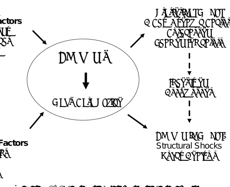
Figure 1 illustrates the nature of the problem for the macroeconomists. In the center is the economy made up of households, firms, and government embedded in physical and institutional structures. To ‘map’ the economy, private firms and public agencies collect an enormous amount of information that is organized and reported by various public and private sources. The most important of these economic indicators are the gross domestic product (over $13.5 trillion in 2007), inflation (the CPI inflation trend has been rather steady around 2-1/2 percent over the last decade), and the number of jobs (payroll employment was about 138 million at the end of 2007). These data are aggregated using thousands of bits of information coming from a sample of the households, firms and government. In this paper we are going to use a much smaller, yet very rich data set

(6)

including 157 time series describing the evolution of production, employment, spending, inflation, interest rates, exchange rates and asset prices. Incoming news about these time series informs us about the short-term stage of the business cycle and expected long-run trends for the major macroeconomic indicators.

On the left side of Figure 1 we sort the factors into those that are common to all the economic indicators—and those that are idiosyncratic. The level of technology in science and industry including management science is a common factor. Recent innovations in computer technology have changed the way everyone keeps track of information and communicates with others. Other common factors include monetary and fiscal policy. Although more difficult to measure, shocks to household preferences for consumption and leisure may also appear to be economy wide. Researchers want to measure these common factors and shocks to them both because they help forecast inflation and output, but also because they are needed to understand how the economy works in order to evaluate the effects of past and proposed policies.

The key assumption underlying the dynamic factor model is that each of the economic indicators is assumed to be driven by a common component made up of a small number of common factors and an idiosyncratic component. Because each of the economic indicators represents the activities of many households and firms, the idiosyncratic shocks estimated in our model may share some common elements. We assume, however, that, unlike the shocks to the common factors, the idiosyncratic shocks do not have economy-wide effects.

On the top right side of Figure 1 we see that a dynamic factor model can be used to estimate a set of common factors that affect all economic time series. The dynamic factor

(7)

model is designed to extract the small number of common factors from a large set of

economic indicators. Stock and Watson (1989) developed coincident and leading indicators of the business cycle using dynamic factor methods.2 Stock and Watson (2002) also use this statistical model to make economic forecasts. Giannone, Reichlin and Small (2005) have developed a dynamic factor model that is used by at the Federal Reserve Board to make short-term forecasts for a large cross-section of data. The estimated common factors are reduced-form constructs—linear combinations of the structural factors that we would like to observe. On the bottom right side, we see that an economic model must be specified in order to identify the structural factors and the structural shocks that are of most interest to policymakers and policy advisors. Here we focus on using the information in the common factors to forecast indicators of inflation and output.

The basic statistical tools used are principal component and factor analysis.3 We observe a large number of time series, x_{i t}_, , i = 1, 2, ... , n; each observed over T periods.

The key assumption in the factor model is that each of the individual xi’s can be

decomposed into a small number of primitive factors which are common to all the x’s and an idiosyncratic componente_{i t}_,,that is uncorrelated with the primitive factors.

, it i t it x =λ′F +e (1) 1 ( ) t t t F = A L F₋ +ε , (2) 1 ( ) it i it t e =ρ L e₋ +υ , (3) 2

The Federal Reserve Bank of Chicago maintains this leading indicator index. See Evans, Liu, and Pham-Kantor (2002).

3

(8)

where Ft =(F1t,...,Frt) ' is a vector containing the q common factors and

0

( ) p_j _j j

A L =

∑

₌ A L is a polynomial in the lag operator, L. The time series x_it is related to the common factors by a vector of factor loadings, λ_i =(λ_i₁,...,λ_ir) '. The disturbance term in (1), e_it, is the idiosyncratic component of x_it, while λ_i'F_t is the common component. If the model is static then it is represented by equation (1). Dynamics may be introduced through the common factor component as in equation (2) and/or through the idiosyncratic component as in equation (3). Boivin and Ng (2005) discuss alternative methods that have been developed to estimate the factors and the factor loadings.4 Then they evaluate the forecasting performance of alternative methods of estimating the dynamic factors. For realistic assumptions about the data, they find that the best forecasting is a simple one that uses the large information set, but does not actually estimate the dynamic factors. We use this method, which involves two steps. The first step is to approximate the factors using the

q largest principal components.5 The second step is to use these principal components in the forecasting model.

Our data matrix has 157 different monthly time series which begin in January 1983 and end 300 months later in December 2007.6 In this particular case, the number of

observations is larger than the number of cross-section units, although that need not be the case. One of the characteristics of this literature is that the number of primitive shocks is usually estimated to be small. Bai and Ng (2007) estimate that there are more than 2 and

4

∑

+ , 1 h t 0 1 where . h t i i h π − π₊ = =

∑

(4)

(10)

and π is the inflation rate as measured the change in the log of the price index and adjusted to be at an annual rate. The leading subscript AO indicates that this is the forecast and the forecast error for the AO model. The subscript t and superscript h indicate that this is the forecast for the average annual inflation rate for h months beginning in month t.

The autoregressive models (AR) have the same dependent variable as above, but the weights on the 12 lags are estimated.7 For the h-month-ahead inflation forecast, the AR model is written as:

12 t 0 1 h h AR i t i AR t i u π φ β π ₋ = = +

∑

+ , (5) We use the same 12 lags for the various horizons and we do not search across lag length for the best in-sample fit when estimating the parameters of the forecasting model. 8

The third set of models includes the data-rich models (DRM). They use the largest principal components as estimates of the factors and adds them to the AR model in

equation (5).9 12 0 , 1 1 1 q m h h DRM t i t i j t k DRM t i j k PC u π φ β π ₋ ₋ = = = = +

∑

+

∑∑

+ (6) The model adds m lags of the first qestimated factors to the AR model. Based on the findings of Bai and Ng (2007a), we expect to find a relatively small number of primitive factors that will be spanned by a combination of primitive factors and their lags. However, in preliminary work for this study, we found that the best models sometimes had more

7

Technically, these are not purely autoregressive models. We could have used an AR model of the 1-month- ahead inflation rate and then iterate over h horizons. However, previous research suggests that forecasting the average over the forecast interval directly as we do here often works better than iterated forecasts in realistic (that is, relatively small) sample sizes.

8

We used 12 lags to take account of seasonal regularities that remain in the data. Hansen (2008) provides theory and evidence to show that using information criteria to choose the best lag length in sample may result in choosing a model that does worst in out-of-sample prediction.

9

(11)

factors and lags than suggested by tests for the number of primitive factors. Therefore, we run models with q taking values from 1 to 7 and m taking values from 1 to 12. All the principal components enter the equation with the same lag length. Note that equation (6) is similar to the forecasting model used by Stock and Watson (2002).

Forecasting Inflation

In this section we report results from forecasting four measures of inflation: the Consumer Price Index (CPI), the chain price index for personal consumption expenditures (PCEPI), and the two versions of these indexes that exclude the prices of their food and energy components, the core CPI and the core PCEPI. The CPI is the most common

measure of inflation and it is commonly used to escalate wages and government benefits. It is also the concept that has been most commonly used as the policy objective by central banks that target inflation. In November 2007 the Federal Reserve began releasing quarterly projections of both total and core measures of PCEPI inflation. The PCEPI is used to compute real personal consumption expenditures in the national income and product accounts.

For our empirical analysis, we chose to begin in January 1983. Our rationale follows the work of those who find a structural break in many macroeconomic variables beginning around that time period. The structural break has been attributed to improved monetary policy, changes in the way firms manufacture and distribute goods, and good luck.10 The onset of this structural break is usually termed the Great Moderation. In this data set we are using data through December 2007. Pseudo out-of-sample forecasts are produced for January 1997 using models that are estimated using current vintage data. The

10

(12)

models (and the principal components) are updated each month, producing recursive inflation forecasts with the final forecast period ending in September 2007. The beginning of the estimation period is fixed, so the number of observations used to estimate the

forecasting equations grows over time. The dependent variable in each of the regressions is an average over the relevant forecast interval. The regressors enter as monthly variables.

The Results. The inflation forecasting results are shown in Table 1 and Figures 2-4. The RMSEs for the 3-month forecast horizon are shown in the top panel of Table 1. The first row reports the results for the AO model. This random walk model does a bit better than the AR model only for Core CPI, but even here, the difference is small. The baseline AR model is shown in the second row. The RMSE for the AR is substantially lower than the AO model for the all-item indexes. The third row reports the RMSEs for the best DRMs. The inclusion of principal components significantly improve the forecasts for the CPI and its core measure, but they do not help forecast the PCEPI or the Core PCEPI.11 Figure 2 shows the RMSEs from all the 3-month-ahead inflation forecasts. The best DRM for the CPI included 3 lags of 7 principal components, a surprising profligate model with 33 estimated parameters. In all the other cases, the best models were smaller, the Core CPI and the PCEPI included just 1 principal component and the best Core PCEPI model included just 1 lag of the first 3 principal components. Figure 2 clearly shows that the DRMs did not contribute much to the 3-month forecasts for the PCEPI or its core measure.

The second panel in Table 1 reports the results for the 12-month-ahead inflation forecasts. Once again the AO model does better than the AR model only in the case of the Core CPI. For all the other experiments reported in the paper, the AO model is worse than

11

The asterisks in Tables 1 and 2 indicate that we can reject the hypothesis that the principal components do not help forecast at the 1 percent critical level using the McCracken (2007) out-of-sample test statistic.

(13)

the AR model which is usually worse than the model that is supplemented with the

principal components. At the 12-month horizon, the information provided by the principal components is statistically significant at the 1-percent level for measures of inflation that we studied. Figure 3 shows that the DRMs do quite well when we extend the model to 12 months. For both measures of CPI inflation, the DRMs with 6 or 7 principal components did well, although the best model for the Core CPI included just 2 principal components with 3 lags of each. There was less improvement in the PCEPI and Core PCEPI, but the improvement was statistically significant.

The bottom panel of Table 1 reports the results for the 24-month-ahead inflation forecasts. The results are similar to those for the 12-month forecasts, but the improvement in the forecasts over the benchmark AR model is larger. The principal components

displayed significant information for all measures of inflation.

Forecasting Real Activity

Next, we use these models to forecast four monthly indicators of real economic activity: (1) the index of coincident indicators; (2) the Purchasing Managers’ Index (PMI), which is a diffusion index that measures activity in the manufacturing sector; (3) real personal consumption expenditures (PCE); and (4) the civilian unemployment rate.12 The index of coincident indicators and real personal consumption expenditures are measured at an annual growth rates, the ISM index is measured in levels and the unemployment rate is measured as the first difference.

12

The coincident index is published by the Conference Board, and it is comprised of (1) nonfarm payroll employment, (2) industrial production, (3) real manufacturing and trade sales, and (4) real personal income less transfer payments. The Purchasing Managers’ Index is published by the Institute for Supply Management

(14)

The results of the out-of sample forecasts for the real variables are presented in table 2. The RMSEs of the random walk models are always the largest relative to the baseline AR and best DRM models. This result was not surprise macroeconomists and forecasters, but we report it to remind readers that the relative good performance of the random walk model in forecasting inflation and asset prices does not carry over into measures of real economic activity. The top panel displays results for the 3-month forecast horizon. The principal components are statistically significant predictors of the PMI and unemployment rate. Figure 4 displays the RMSEs for the specifications of the DRMs of real activity at the 3-month horizon. The best DRM forecast for the PMI included 1 lag of the first 7 principal components. The best DRM forecast of the unemployment rate

included just 1 lag of the first principal component, but all of the DRMs with a few lags did well in predicting the unemployment rate. Including the principal components did not help to forecast the index of coincident indicators or real PCE at the 3-month horizon.

The middle panel of Table 2 reports the results for the 12-month forecast. Figure 6 shows the RMSEs for the specifications of the DRMs of real activity at the 12-month horizon. The best model for the index of coincident indicators has 4 principal components with 9 lags but is no better than the benchmark AR model. The best model for the PMI was the DRM with 4 principal components and 1 lag, but as with the coincident indicators, the principal components do not significantly improve the forecasts. The improvements in the forecasts of real PCE growth and the unemployment rate are statistically significant. Again, the best DRM of the unemployment rate includes just the first principal components, but now includes all 12 lags rather than just the first.

(15)

The bottom panel in Table 2 report results for the 24-month forecasts of real

economic indicators. The best DRM for each of the variables is significantly better than the benchmark AR model. The pattern in the RMSEs for the index of coincident indicators is is similar to pattern in the 12-month results, but the forecasts are better relative to the

benchmark AR model. There is a substantial improvement in the PMI and real PCE forecasts relative to the 12 month results. In both cases, the models with 4 lags and 8 to 10 lags do well. The 24-month unemployment rate models were a bit of an exception in that including more than one principal usually made the DRM model produce a RMSE that was larger than the benchmark AR model. The results for the best out-of-sample forecasting version of Equation (6) are summarized in Table 3.

Conclusion

In this paper we report the results of a simulated out-of-sample forecasting experiment in which we compared 85 models for each of 8 economic indicators over 3 forecasting horizons (for a total of 2040 models). The models were estimated over a period beginning in January 1983 and ending 2 months before the beginning of the forecast

interval. We made 132 forecasts beginning in January 1997 and ending in December 2007. Generally, we find that the data-rich models can be used to improve forecasts of inflation and output. We found that using principal components to estimate the underlying common factors was useful in forecasting the CPI and its core measure at the 3-month horizon and all measures of inflation at the 12- and 24-month horizons. The factor methods were also helpful in predicting real variables. The data rich models were useful in predicting the unemployment rate over all horizons and all the real variables over 24-month horizons.

(16)

In this paper, we used a relatively unrestricted method that did not separately identify the common and idiosyncratic factors. In future research, we plan to identify the common factors and the factor loadings so that we can map source of the information that improves forecast accuracy. We also plan to investigate the benefits of using procedures recommended in Bai and Ng (2007b) for choosing fewer, but informative predictors. They find that one can improve forecast accuracy by using such procedures for each specific variables at each specific forecasting horizon. We are also interested in using dynamic factor methods in combination with economic theory to identify structural economic shocks. This is an emerging area of research that holds promise for doing policy analysis.

(17)

References

Atkeson Andrew, and Lee E. Ohanian, (2001), “Are Phillips Curves Useful for Forecasting Inflation?” FRBMN Quarterly Review 25(1):2-11.

Ahmed Shagil, Andrew Levin and Beth Anne Wilson, (2004), “Recent U.S.

Macroeconomic Stability: Good Policies, Good Practices, or Good Luck?” The Review of Economics and Statistics 86(3):824-32.

Bai, Jushan, and Serena Ng. (2007a) “Determining the Number of Primitive Shocks in Factor Models,” Journal of Business and Economic Statistics 25(1), 52-60. Bai, Jushan, and Serena Ng. (2007b) “Forecasting Economic Time Series Using Targeted

Predictors,” Working paper University of Michigan, November 14. Forthcoming in

Journal of Econometrics.

Bai, Jushan, and Serena Ng. (2005) “Understanding and Comparing Factor-Based Forecasts,” International Journal of Central Banking 1(3), 117-151.

Bernanke Ben S., (1986), “Alternative Explanations of the Money-Income Correlation,”

Carnegie-Rochester Conference Series on Public Policy 25:49-100.

Bernanke Ben S., and Jean Boivin, (2003), “Monetary Policy in a Data-Rich Environment,”

Journal of Monetary Economics, 50(3):525-546.

Bernanke, Ben, Jean Boivin, and Piotr Eliasz (2005), “Measuring Monetary Policy: A Factor Augmented Vector Autoregressive (FAVAR) Approach,” Quarterly Journal of Economics 120(1):387-422.

Boivin, Jean, and Marc P. Giannoni (2006), “DSGE Models in a Data-Rich Environment,” Manuscript presented on July 6 in the Macro Seminar Series at the Federal Reserve Bank of St. Louis.

Boivin, Jean, and Serena Ng. (2005), “Understanding and Comparing Factor-Based Forecasts” International Journal of Central Banking 1 (December), 117-149. Eickmeier, Sandra, and Christina Ziegler. (2006), “How Good Are Dynamic Factor Models

at Forecasting Output and Inflation? A Meta-Analytic Approach,” Deutsche Bundesbank Discussion Paper Sereies 2006-42.

Evans, Chales L., Chin Te Liu, and Genevieve Pham-Kanter, (2002), “The 2001 Recession and the Chicago Fed National Activity Index: Identifying Cycle Turning Points,” Federal Reserve Bank of Chicago Economic Perspectives (Third Quarter), 26-43.

(18)

Evans, Charles L., and David A. Marshall (2006), “Fundamental Economic Shocks and the Macroeconomy,” manuscript October 15, 2006 version, Federal Reserve Bank of Chicago.

Forni, Mario, and Marco Lippi, (2001), “The Generalized Dynamic Factor Model: Representation Theory,” Econometric Theory, 17, 1113-1141.

Forni, Mario, Marc Hallin, Marco Lippi, and Lucrezia Reichlin, (2000), “The Generalized Dynamic-Factor Model: Identification and Estimation,” Review of Economics and Statistics 82(4), 540-554.

Giannone, Domenica, and Lucrezia Reichlin, (2006), “Does Information Help Recovering Sturctural Shocks From Past Observations?” European Central Bank Working Paper Series No. 632, May.

Giannone, Domenico, Lucrezia Reichlin, and Luca Sala, (2005), “Monetary Policy in real Time,” in Mark Gertler and Kenneth Rogoff, eds., NBER Macroeconomics Annual 2004, 161-200. MIT Press.

Giannone, Domenico, Lucrezia Reichlin, and David Small, (2005), “Nowcasting: The Real Time Informational Content of Macroeconomic Data Releases’’forthcoming in

Journal of Monetary Economics, see

http://homepages.ulb.ac.be/~dgiannon/Nowcasting.pdf

Hansen, Peter R. (2008), “In-Sample and Out-of-Sample Fit: Their Joint Distribution and its Implications for Model Selection and Model Averaging,” Working Paper, Stanford University, March 18.

King, Robert G., (1986), “Money and Business Cycles: Comments on Bernanke and Related Literature,” Carnegie-Rochester Conference Series on Public Policy 25, 101-116.

McConnell, Margaret M., and Gabriel Perez Quiros, (2000), “Output Fluctuations in the United States: What Has Changed Since the Early 1980’s?” American Economic Review 90(5), 1464-76.

McCracken, Michael W., (2007), ''Asymptotics for Out-of-Sample Tests of Granger Causality,'' Journal of Econometrics, vol. 140 (October), 719-752.

(19)

Schumacher, Christian (2007), “Forecasting German GDP Using Alternative Factor Models Based on Large Datasets,” Journal of Forecasting 26, 271-302.

Stock, James H., and Mark W. Watson, (2005a), “Implications of Dynamic Factor Models for VAR Analysis,” NBER Working Paper 11467.

_______, (2005b), “Has Inflation Become Harder to Forecast?” Paper presented at the conference, “Quantitative Evidence on Price Determination,” Board of Governors of the Federal Reserve System, September 29-30, Washington D.C.

_______, (2002), “Macroeconomic Forecasting Using Diffusion Indexes,” Journal of Business and Economic Statistics 20: 147-162.

_______, (1999), “Forecasting Inflation,” Journal of Monetary Economics 44:293-335. _______, (1989), “New Indexes of Coincident and Leading Economic Indicators,” NBER

Macroeconomics Annual, 351-393.

Taylor, John, (1998), “Monetary Policy and the Long Boom,” Review, Federal Reserve Bank of St. Louis, 80(6):3-11.

(20)

Table 1: Comparing Data-Rich Models of Inflation with Simple Rules (RMSEs in percent at annual rates)

3 month CPI Core CPI PCEPI Core PCE

AO 2.03 0.61 1.54 0.69 AR(12) 1.76 0.62 1.44 0.67 DRM 1.67* 0.59* 1.42 0.67 12 month AO 1.15 0.48 0.84 0.40 AR(12) 0.99 0.49 0.77 0.38 DRM 0.90* 0.43* 0.71* 0.36* 24 month AO 1.00 0.51 0.78 0.39 AR(12) 0.80 0.50 0.69 0.36 DRM 0.63* 0.39* 0.59* 0.33*

* indicates that the DRM model is significantly more accurate than the AR(12) model at the 1-percent critical level.

(21)

Table 2: Comparing Data-Rich Models of Economic Activity with Simple Rules (RMSEs in percent at annual rates for the Coincident Indicators and Real PCE)

3 month

Coincident

Indicators PMI Real PCE

Unemployment Rate AO 1.65 4.21 2.19 0.070 AR(12) 1.56 2.43 2.02 0.068 DRM 1.55 2.32* 2.03 0.062* 12 month AO 1.54 4.94 1.17 0.055 AR(12) 1.37 3.18 0.97 0.046 DRM 1.36 3.14 0.92* 0.040* 24 month AO 1.71 4.86 1.19 0.058 AR(12) 1.34 2.73 0.87 0.040 DRM 1.22* 2.43* 0.61* 0.038* * reject the null hypothesis that the factors do not Granger cause the forecast variable at the 1-percent critical level.

Note: PMI is measured as the average level over the forecast horizon. The unemployment rate is measured as the average monthly change over the forecast horizon.

(22)

Table 3

What's the Best Data-Rich Model?

Inflation Real Activity

3-month-ahead forecasts q* m q m

CPI 7 3 Coincident Indicators 1 1

Core CPI 1 2 ISM PMI 7 1

PCEPI 1 9 Real PCE 1 1

Core PCEPI 3 1 Unemployment Rate 1 1

12-month-ahead forecasts

24-month-ahead forecasts

(23)

A Few

Common Factors

Technology

Preferences

Policy

Many

Idiosyncratic

Factors

Households

Firms

Sectors

Many Data Series

Economy

Statistical Model

A Few Dynamic Factors

Forecasting

Leading Indicators

Economic Model

s

Structural Shocks

Policy Analysis

Figure 1. Schematic for data-rich models

Identifying

Assumptions

(24)

Figure 2

Inflation Forecast Accuracy: RMSEs of 3-Month-Ahead Forecasts*

* Each group of principal components includes RMSEs from models with lags from 1 to 12. 22

CPI 1.5% 1.6% 1.7% 1.8% 1.9% 2.0% 2.1% AR (12) 1 P rin Com p 2 P rin Com ps 3 P rin Com ps 4 P rin Com ps 5 P rin Com ps 6 P rin Com ps 7 P rin Com ps Core CPI 0.50% 0.55% 0.60% 0.65% 0.70% 0.75% AR (12) 1 P rin Com p 2 P rin Com ps 3 P rin Com ps 4 P rin Com ps 5 P rin Com ps 6 P rin Com ps 7 P rin Com ps PCEPI 1.3% 1.4% 1.4% 1.5% 1.5% 1.6% 1.6% AR (12) 1 P rin Com p 2 P rin Com ps 3 P rin Com ps 4 P rin Com ps 5 P rin Com ps 6 P rin Com ps 7 P rin Com ps Core PCEPI 0.5% 0.6% 0.7% 0.8% 0.9% AR (12) 1 P rin Com p 2 P rin Com ps 3 P rin Com ps 4 P rin Com ps 5 P rin Com ps 6 P rin Com ps 7 P rin Com ps

(25)

Figure 3

CPI 0.8% 0.9% 1.0% 1.1% 1.2% 1.3% AR (12) 1 P rin Com p 2 P rin Com ps 3 P rin Com ps 4 P rin Com ps 5 P rin Com ps 6 P rin Com ps 7 P rin Com ps Core CPI 0.40% 0.45% 0.50% 0.55% 0.60% AR (12) 1 P rin Com p 2 P rin Com ps 3 P rin Com ps 4 P rin Com ps 5 P rin Com ps 6 P rin Com ps 7 P rin Com ps PCEPI 0.6% 0.7% 0.7% 0.8% 0.8% 0.9% 0.9% 1.0% 1.0% AR (12) 1 P rin Com p 2 P rin Com ps 3 P rin Com ps 4 P rin Com ps 5 P rin Com ps 6 P rin Com ps 7 P rin Com ps Core PCEPI 0.30% 0.35% 0.40% 0.45% 0.50% AR (12) 1 P rin Com p 2 P rin Com ps 3 P rin Com ps 4 P rin Com ps 5 P rin Com ps 6 P rin Com ps 7 P rin Com ps

(26)

Figure 4

CPI 0.6% 0.7% 0.8% 0.9% 1.0% AR (12) 1 P rin Com p 2 P rin Com ps 3 P rin Com ps 4 P rin Com ps 5 P rin Com ps 6 P rin Com ps 7 P rin Com ps Core CPI 0.30% 0.35% 0.40% 0.45% 0.50% 0.55% AR (12) 1 P rin Com p 2 P rin Com ps 3 P rin Com ps 4 P rin Com ps 5 P rin Com ps 6 P rin Com ps 7 P rin Com ps PCEPI 0.5% 0.6% 0.7% 0.8% AR (12) 1 P rin Com p 2 P rin Com ps 3 P rin Com ps 4 P rin Com ps 5 P rin Com ps 6 P rin Com ps 7 P rin Com ps Core PCEPI 0.30% 0.35% 0.40% 0.45% AR (12) 1 P rin Com p 2 P rin Com ps 3 P rin Com ps 4 P rin Com ps 5 P rin Com ps 6 P rin Com ps 7 P rin Com ps

(27)

Figure 5

Economic Activity Forecast Accuracy: RMSEs of 3-Month-Ahead Forecasts*

Coincident Indicators 1.4% 1.5% 1.6% 1.7% 1.8% 1.9% 2.0% 2.1% AR (12) 1 P rin Com p 2 P rin Com ps 3 P rin Com ps 4 P rin Com ps 5 P rin Com ps 6 P rin Com ps 7 P rin Com ps ISM PMI 2.2 2.3 2.4 2.5 2.6 2.7 2.8 2.9 3.0 AR (12) 1 P rin Com p 2 P rin Com ps 3 P rin Com ps 4 P rin Com ps 5 P rin Com ps 6 P rin Com ps 7 P rin Com ps Real PCE 1.7% 1.9% 2.1% 2.3% 2.5% 2.7% 2.9% 3.1% 3.3% AR (12) 1 P rin Com p 2 P rin Com ps 3 P rin Com ps 4 P rin Com ps 5 P rin Com ps 6 P rin Com ps 7 P rin Com ps Unemployment Rate 0.060 0.063 0.066 0.069 0.072 0.075 0.078 AR (12) 1 P rin Com p 2 P rin Com ps 3 P rin Com ps 4 P rin Com ps 5 P rin Com ps 6 P rin Com ps 7 P rin Com ps

(28)

Figure 6

Coincident Indicators 1.2% 1.3% 1.4% 1.5% 1.6% 1.7% AR (12) 1 P rin Com p 2 P rin Com ps 3 P rin Com ps 4 P rin Com ps 5 P rin Com ps 6 P rin Com ps 7 P rin Com ps ISM PMI 3.0 3.1 3.2 3.3 3.4 3.5 3.6 3.7 3.8 AR (12) 1 P rin Com p 2 P rin Com ps 3 P rin Com ps 4 P rin Com ps 5 P rin Com ps 6 P rin Com ps 7 P rin Com ps Real PCE 0.8% 0.9% 1.0% 1.1% 1.2% 1.3% 1.4% AR (12) 1 P rin Com p 2 P rin Com ps 3 P rin Com ps 4 P rin Com ps 5 P rin Com ps 6 P rin Com ps 7 P rin Com ps Unemployment Rate 0.038 0.040 0.042 0.044 0.046 0.048 0.050 0.052 AR (12) 1 P rin Com p 2 P rin Com ps 3 P rin Com ps 4 P rin Com ps 5 P rin Com ps 6 P rin Com ps 7 P rin Com ps

(29)

Figure 7

Coincident Indicators 1.1% 1.2% 1.3% 1.4% 1.5% 1.6% AR (12) 1 P rin Com p 2 P rin Com ps 3 P rin Com ps 4 P rin Com ps 5 P rin Com ps 6 P rin Com ps 7 P rin Com ps ISM PMI 2.3 2.4 2.5 2.6 2.7 2.8 2.9 3.0 AR (12) 1 P rin Com p 2 P rin Com ps 3 P rin Com ps 4 P rin Com ps 5 P rin Com ps 6 P rin Com ps 7 P rin Com ps Real PCE 0.5% 0.6% 0.6% 0.7% 0.7% 0.8% 0.8% 0.9% 0.9% AR (12) 1 P rin Com p 2 P rin Com ps 3 P rin Com ps 4 P rin Com ps 5 P rin Com ps 6 P rin Com ps 7 P rin Com ps Unemployment Rate 0.036 0.038 0.040 0.042 0.044 0.046 0.048 AR (12) 1 P rin Com p 2 P rin Com ps 3 P rin Com ps 4 P rin Com ps 5 P rin Com ps 6 P rin Com ps 7 P rin Com ps

(30)

Appendix

Data Used in the DFM Analysis, Their Transformation and Their Source

Description

Real Output and Income Transformation Source

1 IP: Total Index (SA, 2002=100) DLN FRB

2 IP: Final Products and Nonindustrial Supplies (SA, 2002=100) DLN FRB

3 IP: Final Products {Mkt Group} (SA, 2002=100) DLN FRB

4 IP: Consumer Goods (SA, 2002=100) DLN FRB

5 IP: Durable Consumer Goods (SA, 2002=100) DLN FRB

6 IP: Nondurable Consumer Goods (SA, 2002=100) DLN FRB

7 IP: Business Equipment (SA, 2002=100) DLN FRB

8 IP: Materials (SA, 2002=100) DLN FRB

9 IP: Durable Materials (SA, 2002=100) DLN FRB

10 IP: Nondurable Materials (SA, 2002=100) DLN FRB

11 IP: Manufacturing (SIC) (SA, 2002=100) DLN FRB

12 IP: Durable Manufacturing [NAICS] (SA, 2002=100) DLN FRB

13 IP: Nonindustrial Supplies (SA, 2002=100) DLN FRB

14 IP: Nondurable Manufacturing [NAICS] (SA, 2002=100) DLN FRB

15 Industrial Production: Mining (SA, 2002=100) DLN FRB

16 IP: Consumer Energy Products: Residential Utilities (SA, 2002=100) DLN FRB 17 IP: Consumer Energy Products: Fuels (SA, 2002=100) DLN FRB

18 IP: Electric and Gas Utilities (SA, 2002=100) DLN FRB

19 IP: Motor Vehicle Assemblies (SAAR, Mil.Units) DLN FRB

20 ISM Mfg: Production Index (SA, 50+ = Econ Expand) LV ISM

21 Capacity Utilization: Manufacturing [SIC] (SA, % of Capacity) DLV FRB

22 Real Personal Income (SAAR, Bil.Chn.2000$) DLN BEA/H

23 Real Personal Income Less Transfer Payments (SAAR, Bil.Chn.2000$) DLN BEA/H 24 Real Disposable Personal Income (SAAR, Bil.Chn.2000$) DLN BEA

Employment and Hours

25 Index of Help-Wanted Advertising in Newspapers (SA,1987=100) DLN CNFBOARD 26 Ratio: Help-Wanted Advertising in Newspapers/Number Unemployed (SA) DLN CB/BLS/H 27 Civilian Employment: Sixteen Years & Over (SA, Thousands) DLN BLS 28 Civilian Employment: Nonagricultural Industries: 16 yr + (SA, Thous) DLN BLS

29 Civilian Unemployment Rate: 16 yr + (SA, %) DLV BLS

30 Civilian Unemployment Rate: Men, 25-54 Years (SA, %) DLV BLS 31 Average {Mean} Duration of Unemployment (SA, Weeks) DLV BLS 32 Civilians Unemployed for Less Than 5 Weeks (SA, Thous.) DLN BLS

33 Civilians Unemployed for 5-14 Weeks (SA, Thous.) DLN BLS

34 Civilians Unemployed for 15 Weeks and Over (SA, Thous.) DLN BLS 35 Civilians Unemployed for 15-26 Weeks (SA, Thous.) DLN BLS 36 Civilians Unemployed for 27 Weeks and Over (SA, Thous.) DLN BLS 37 Unemployment Insurance: Initial Claims, State Programs (SA, Thous) DLV DOL

38 All Employees: Total Nonfarm (SA, Thous) DLN BLS

39 All Employees: Total Private Industries (SA, Thous) DLN BLS 40 All Employees: Goods-producing Industries (SA, Thous) DLN BLS

41 All Employees: Mining (SA, Thous) DLN BLS

(31)

43 All Employees: Manufacturing (SA, Thous) DLN BLS 44 All Employees: Durable Goods Manufacturing (SA, Thous) DLN BLS 45 All Employees: Nondurable Goods Manufacturing (SA, Thous) DLN BLS 46 All Employees: Service-providing Industries (SA, Thous) DLN BLS 47 All Employees: Trade, Transportation & Utilities (SA, Thous) DLN BLS

48 All Employees: Wholesale Trade (SA, Thous) DLN BLS

49 All Employees: Retail Trade (SA, Thous) DLN BLS

50 All Employees: Financial Activities (SA, Thous) DLN BLS

51 All Employees: Government (SA, Thous) DLN BLS

52 Aggregate Weekly Hours Index: Total Private Industries (SA, 2002=100) DLN BLS 53 Average Weekly Hours: Goods-producing Industries (SA, Hrs) LV BLS 54 Average Weekly Hours: Overtime: Manufacturing (SA, Hrs) DLV BLS

55 Average Weekly Hours: Manufacturing (SA, Hrs) DLV BLS

56 ISM Mfg: Employment Index (SA, 50+ = Econ Expand) LV ISM

Real Retail, Manufacturing and Trade Sales

57 Manufacturing & Trade Sales (SA, Mil.Chn.2000$) DLN CNFBOARD 58 Manufacturing & Trade Inventories (EOP, SA, Bil.Chn.2000$) DLN CNFBOARD 59 Mfg & Trade: Inventories/Sales Ratio (SA, Chn.2000$) DLN CNFBOARD 60 Manufacturers' Shipments of Mobile Homes (SAAR, Thous.Units) LN CENSUS

61 Real Retail Sales & Food Services DLN AUTHORS

Inventories and Orders

62 ISM Mfg: Inventories Index (SA, 50+ = Econ Expand) LV ISM

63 ISM Mfg: New Orders Index (SA, 50+ = Econ Expand) LV ISM

64 Mfrs New Orders: Durable Goods (SA, Mil.Chn.2000$) DLN CNFBOARD 65 Manufacturers New Orders: Nondefense Capital Goods (SA, Mil. 1982$) DLN CNFBOARD 66 Mfrs Unfilled Orders: Durable Goods (SA, EOP, Mil.Chn.2000$) DLN CNFBOARD

Consumption

67 Real Personal Consumption Expenditures: Durable Goods (SAAR, Bil.Chn.2000$) DLN BEA 68 Real Personal Consumption Expenditures: Nondurable Goods (SAAR, Bil.Chn.2000$) DLN BEA 69 Real Personal Consumption Expenditures: Services (SAAR, Bil.Chn.2000$) DLN BEA 70 Real Personal Consumption Expenditures (SAAR, Bil.Chn.2000$) DLN BEA

Housing Starts and Sales

71 Housing Starts (SAAR, Thous.Units) LN CENSUS

72 Housing Starts: Northeast (SAAR, Thous.Units) LN CENSUS

73 Housing Starts: Midwest (SAAR, Thous.Units) LN CENSUS

74 Housing Starts: South (SAAR, Thous.Units) LN CENSUS

75 Housing Starts: West (SAAR, Thous.Units) LN CENSUS

76 New Pvt Housing Units Authorized by Building Permit (SAAR, Thous.Units) LN CENSUS 77 Housing Units Authorized by Permit: Northeast (SAAR, Thous.Units) LN CENSUS 78 Housing Units Authorized by Permit: Midwest (SAAR, Thous.Units) LN CENSUS 79 Housing Units Authorized by Permit: South (SAAR, Thous.Units) LN CENSUS 80 Housing Units Authorized by Permit: West (SAAR, Thous.Units) LN CENSUS 81 Total Public Construction (SAAR, Mil. Chained 1996$) DLN AUTHORS 82 Private Construction: Nonresidential (SAAR, Mil. Chained 1996$ DLN AUTHORS

(32)

Stock Prices

83 Stock Price Index: Standard & Poor's 500 Composite (1941-43=10) DLN WSJ 84 Stock Price Index: Standard & Poor's 500 Industrials (1941-43=10) DLN FINTIMES

85 S&P: Composite 500, Dividend Yield (%) DLV S&P/H

86 S&P: 500 Composite, P/E Ratio, 4-Qtr Trailing Earnings (Ratio) DLN S&P/H 87 Stock Price Index: NASDAQ Composite (Feb-5-71=100) DLN WSJ

Exchange Rates

88 Nominal Broad Trade-Weighted Exchange Value of the US$ (Jan-97=100) DLN FRB 89 Real Broad Trade-Weighted Exchange Value of the US$ (Mar-73=100) DLN FRB

90 Foreign Exchange Rate: Switzerland (Franc/US$) DLN FRB

91 Foreign Exchange Rate: Japan (Yen/US$) DLN FRB

92 Foreign Exchange Rate: United Kingdom (US$/Pound) DLN FRB

93 Foreign Exchange Rate: Canada (C$/US$) DLN FRB

Interest Rates

94 Federal Funds [effective] Rate (% p.a.) DLV FRB

95 3-Month Nonfinancial Commercial Paper (% per annum) DLV FRB 96 3-Month Treasury Bills, Secondary Market (% p.a.) DLV FRB 97 6-Month Treasury Bills, Secondary Market (% p.a.) DLV FRB 98 1-Year Treasury Bill Yield at Constant Maturity (% p.a.) DLV FRB 99 5-Year Treasury Note Yield at Constant Maturity (% p.a.) DLV FRB 100 10-Year Treasury Note Yield at Constant Maturity (% p.a.) DLV FRB 101 Moody's Seasoned Aaa Corporate Bond Yield (% p.a.) DLV FRB 102 Moody's Seasoned Baa Corporate Bond Yield (% p.a.) DLV FRB

Yield Spreads

Eight Series Listed Below Minus the Federal Funds Rate

103 3-Month Nonfinancial Commercial Paper (% per annum) LV FRB 104 3-Month Treasury Bills, Secondary Market (% p.a.) LV FRB 105 6-Month Treasury Bills, Secondary Market (% p.a.) LV FRB 106 1-Year Treasury Bill Yield at Constant Maturity (% p.a.) LV FRB 107 5-Year Treasury Note Yield at Constant Maturity (% p.a.) LV FRB 108 10-Year Treasury Note Yield at Constant Maturity (% p.a.) LV FRB 109 Moody's Seasoned Aaa Corporate Bond Yield (% p.a.) LV FRB 110 Moody's Seasoned Baa Corporate Bond Yield (% p.a.) LV FRB

Money and Credit Quantity Aggregates

111 Money Stock: M1 (SA, Bil.$) DLN FRB

112 Money Stock: M2 (SA, Bil.$) DLN FRB

113 Money Stock: Institutional Money Funds (SA, Bil.$) DLN FRB

114 Real Money Stock: M2 (SA, Bil.Chn.2000$) DLN FRB/BEA/H

St. Louis Adjusted Monetary Base

115 Adj Monetary Base inc Deposits to Satisfy Clearing Bal Contracts (SA, Bil.$) DLN FRBSTL 116 Adjusted Reserves of Depository Institutions (SA, Mil.$) DLN FRB 117 Adjusted Nonborrowed Reserves of Depository Institutions (SA, Mil.$) DLN FRB 118 Real Commercial and Industrial Loans Outstanding (SA, Mil.Chn.2000$) DLN FRB/BEA/H

(33)

119 C & I Loans in Bank Credit: All Commercial Banks (SA, Bil.$) DLN FRB 120 Consumer Revolving Credit Outstanding (EOP, SA, Bil.$) DLN FRB 121 Nonrevolving Consumer Credit Outstanding (EOP, SA, Bil.$) DLN FRB 122 Ratio: Consumer Installment Credit to Personal Income (SA, %) DLV FRB/BEA/H

Price Indexes and Wages

123 PPI: Finished Goods (SA, 1982=100) DLN BLS

124 PPI: Finished Consumer Goods (SA, 1982=100) DLN BLS

125 PPI: Finished Goods: Capital Equipment (SA, 1982=100) DLN BLS 126 PPI: Intermediate Materials, Supplies and Components (SA, 1982=100) DLN BLS 127 PPI: Crude Materials for Further Processing (SA, 1982=100) DLN BLS 128 PPI: Fuels and Related Products and Power (NSA, 1982=100) DLN BLS 129 PPI: Industrial Commodities Less Fuels & Power (NSA, 1982=100) DLN BLS 130 Reuters/Jefferies CRB Futures Price Index: All Commodities (1967=100) DLN CRB

131 CPI-U: All Items (SA, 1982-84=100) DLN BLS

132 CPI-U: Apparel (SA, 1982-84=100) DLN BLS

133 CPI-U: Transportation (SA, 1982-84=100) DLN BLS

134 CPI-U: Medical Care (SA, 1982-84=100) DLN BLS

135 CPI-U: Housing (SA, 1982-84=100) DLN BLS

136 FRB Cleveland Median CPI (SAAR, %chg) LV FRBCLV

137 CPI-U: Commodities (SA, 1982-84=100) DLN BLS

138 CPI-U: Durables (SA, 1982-84=100) DLN BLS

139 CPI-U: Services (SA, 1982-84=100) DLN BLS

140 CPI-U: All Items Less Food and Energy (SA, 1982-84=100) DLN BLS

141 CPI-U: All Items Less Food (SA, 1982-84=100) DLN BLS

142 CPI-U: All Items Less Shelter (SA, 1982-84=100) DLN BLS

143 CPI-U: All Items Less Medical Care (SA, 1982-84=100) DLN BLS

144 PCE: Chain Price Index (SA, 2000=100) DLN BEA

145 PCE: Durable Goods: Chain Price Index (SA, 2000=100) DLN BEA 146 PCE: Nondurable Goods: Chain Price Index (SA, 2000=100) DLN BEA

147 PCE: Services: Chain Price Index (SA, 2000=100) DLN BEA

148 PCE less Food & Energy: Chain Price Index (SA, 2000=100) DLN BEA 149 Avg Hourly Earnings: Goods-producing Industries (SA, $/Hr) DLN BLS

150 Avg Hourly Earnings: Construction (SA, $/Hr) DLN BLS

151 Avg Hourly Earnings: Manufacturing (SA, $/Hr) DLN BLS

152 New 1-Family Houses: Median Sales Price (Dollars) DLN CENSUS 153 NAR Median Sales Price: Existing 1-Family Homes, United States ($) DLN REALTOR

Miscellaneous

154 ISM Mfg: Supplier Deliveries Index (SA, 50+ = Slower) LV ISM

155 University of Michigan: Inflation Expectations LV UMICH/FRED

156 University of Michigan: Consumer Expectations (NSA, Q1-66=100) DLV UMICH 157 ISM Mfg: PMI Composite Index (SA, 50+ = Econ Expand) LV ISM

Addenda:

Nomenclature: By Transformation DLN: Change in logs, annualized DLV: Change in levels

(34)

Nomenclature: By Data Source AUTHORS: Calculation by authors BEA: Bureau of Economic Analysis BLS: Bureau of Labor Statistics

CENSUS: U.S. Department of the Census CB/CNFBOARD: The Conference Board CRB: Commodity Research Bureau DOL: Department of Labor FINTIMES: Financial Times

FRB: Board of Governors of the Federal Reserve System FRBCLV: Federal Reserve Bank of Cleveland

FRBSTL: Federal Reserve Bank of St. Louis

FRED: Federal Reserve Economic Data, Federal Reserve Bank of St. Louis H: Haver Analytics

IP: Industrial Production

ISM: Institute for Supply Management REALTOR: National Association of Realtors S&P: Standard & Poors

UMICH: University of Michigan Survey Research Center WSJ: The Wall Street Journal