Tan, K.J. B., Wang, P. C. and Srigrarom, S. (2017) Computational Modelling of Wing
Downwash Profile with Reynolds-Averaged and Delayed Detached-Eddy Simulations.
In: 23rd AIAA Computational Fluid Dynamics Conference, Denver, CO, USA, 05-09
Jun 2017, ISBN 9781624105067.
There may be differences between this version and the published version. You are
advised to consult the publisher’s version if you wish to cite from it.
http://eprints.gla.ac.uk/142068/
Deposited on: 4 July 2017
Enlighten – Research publications by members of the University of Glasgow
http://eprints.gla.ac.uk
Computational Modelling of Wing Downwash Profile with
Reynolds-Averaged and Delayed Detached-Eddy
Simulations
K. J. Benjamin Tan1University of Glasgow Singapore, Singapore 139661
P. C. Wang2
Singapore Institute of Technology, Singapore 138683 and
S. Srigrarom3
University of Glasgow Singapore, Singapore 139661
This paper describes the computational model to predict downwash for a conventional fixed wing configuration at flight scales (ReMAC = 2.26 × 10⁷). The lack of resolution in the downwash wake region resulted in an over-dissipation of the turbulent behaviour of airflow in the wing’s wake. This artificially inflates the effectiveness of the horizontal stabilizer where an over-prediction of pitch stiffness was observed. To resolve this over-dissipation, both the Reynolds-Averaged and Delayed Detached-Eddy Simulation methodology were adopted to accurately capture the downwash profile leaving the wing. Comparisons between the estimation of wall shear stresses and viscous wall unit against a ‘first-cut’ simulation are made and discussed. Fundamental features of the downwash profile including the spatial and temporal scales used for the mesh are also presented and detailed in this paper.
Nomenclature
𝐶 = Courant number
𝐶𝑓 = coefficient of friction
𝑓𝑑 = blending factor
𝑆̃ = source term
𝜏𝑤 = wall shear stress
𝑢 = component of velocity parallel to wall Uz = vertical velocity component
𝜇 = dynamic viscosity
𝜇𝑡 = turbulent viscosity
𝜈̃ = modified turbulent viscosity
Δ = subgrid length scale
∆𝑡 = time step
𝜀 = downwash angle
𝛼 = angle of attack
All other symbols have their usual meaning and positive convention follows the aircraft principal axes (front, right, down) with the origin at wing leading edge.
I.
Introduction
Longitudinal stability is the most important flight characteristic of an aircraft where prior to any flights, its stability must be ascertained.1 As the horizontal stabilizer for a conventional fixed wing configuration is the dominant
contributor to pitch stability, the assessment of its effectiveness and local airflow is crucial.2 When the tail lies within
the wake of the wings, the impingement of airflow from the wing’s wake alters the tail’s performance. The effectiveness of the horizontal stabilizers in this situation can be theoretically treated by introducing a tail efficiency factor where a ratio between the freestream and local horizontal tail
dynamic pressures is taken.2 Typical values are 0.8 to 1.2.3 This
downward deflection of airflow alters the effective angle of attack for the horizontal stabilizer which affects the amount of force and moments generated by the tail for pitch. If the vertical component(s) of this field can be numerically captured, the downwash angle can be estimated. This effect of downwash on the tail is significant and must not be neglected. Having the effective angle of attack at the tail altered subsequently affects the aircraft’s trim. These interactions can only be assessed by use of simulations or experiments.4
From past preliminary studies on aerodynamic data acquisition,5 an over-prediction was observed for pitching
moment coefficients 𝐶𝑀 across angles of attack, represented by a steeper 𝐶𝑀𝛼 in comparison with published wind
tunnel data.6 This over-prediction of the pitch stiffness was attributed to the lack of resolution in the region of wing
downwash, which in a conventional fixed wing configuration, would affect the modelled effectiveness of the horizontal stabilizer. The lack of foresight to capture these fore-aft aerodynamic interactions with sufficiently fine mesh led to numerical dissipation of turbulent properties of the airflow. The motivation and importance of capturing results in this region branches from the observations made from these preliminary past work.5
For a finite wing, the two prominent flow features are the wing tip vortices and vortex sheet.7 Emphasis here is
placed on the downwash along the vortex sheet. This wake has been the subject of study by experimental methods and formulated to predict downwash angles and wake characteristics.8,9 The formulated results from these work show that
the wake exhibits different characteristics along the span-wise direction of the wing being studied and for practical purposes, the mutual interference between the fuselage and wing or tail has to be considered.
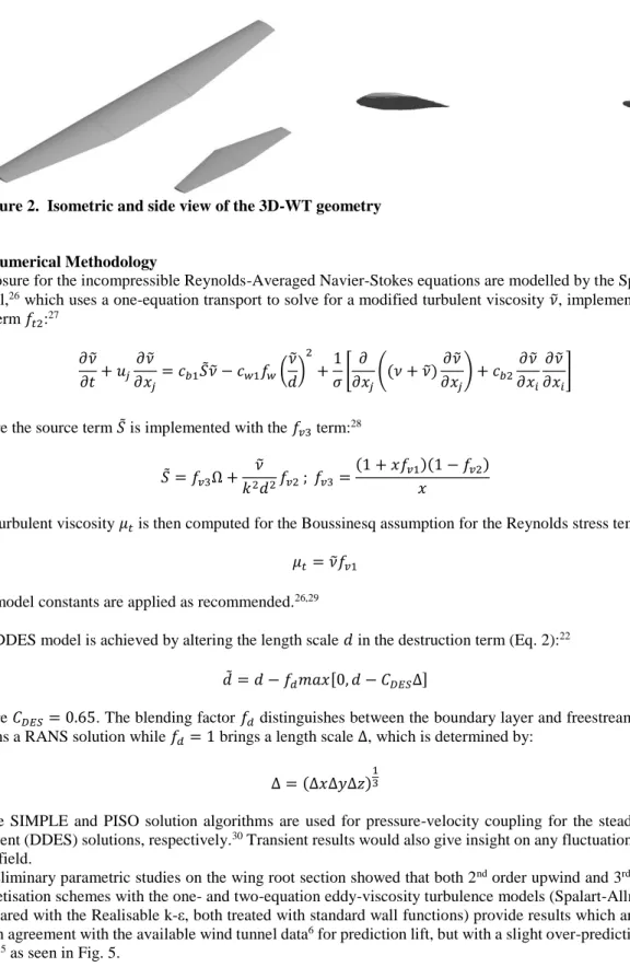
A focused geometry shown in Fig. 2 is used by exclusively modelling the plain wing and tail. This was first explored from the approximation that lift for the wing-body combination can be represented by only the wings but inclusive of the midsection masked by the fuselage.5,10 This same principle is applied to the horizontal stabilizers which are
analogous to the wings but where their contribution are towards stability. However, the presence of the midsection of the horizontal stabilizers that was initially masked by the fuselage are also modelled. The benefit of such a simplified model in addition to exploiting symmetry, is that it can make the entire meshing and simulation process much more economical, especially when the flow conditions are at flight Reynolds numbers. This range of airspeed is observed for the actual aircraft that the geometry here is modelled after (0.19 < M < 0.45).11,12 The wind tunnel data that is used
for validation here was also corrected for these freestream velocities (M = 0.23).6
The absence of the fuselage has a considerable impact on the stability and aerodynamics of the geometry as a fuselage typically shifts the aerodynamic centre aft, thus a Wing-Tail geometry is likely to be longitudinally stiffer than a Wing-Body-Tail configuration.13 In the context of a wing-tail only configuration, this makes the choice of
location to be studied challenging as computationally modelling of such comprehensive datasets9 would be exhaustive.
Furthermore, results involving the midspan (along aircraft symmetry plane) are likely to be interfered by a fuselage. Hence, results for the downwash are taken at a wing outboard station of 20% wing span (which corresponds to approximately 25% tail span) from the aircraft centerline.
The studies on downwash and wake behind airfoils have indicated that empirical methods are sufficient for use as a basis for downwash computation and wing tip vortices may be neglected for the purposes of downwash studies.8
Importantly, the vertical displacement of the vortex sheet due to downflow must be taken into consideration for calculations. This vertical velocity is quantified in the following studies.9 A characteristic pattern of the up and
downwash of vertical velocity components along the longitudinal direction around the wing is shown in Fig. 1. The vertical quantities of velocity are critical in estimating downwash angles based on the freestream. Resolving for flow fields trailing from the wings and how the physical presence of the tail affects this characteristic downwash profile are the focus, and require refinements to the mesh to capture these features. These are in the form of a mesh sensitivity test.
A brief assessment of the wing tip vortex size is also done to determine the profile of vortex tangential velocities towards the tail. At this short distance, it is very likely that the vortex is still developing and shows that the wing tip Figure 1. Qualitative pattern of up and downwash induced by wing vorticity.2
vortex has little effect on the tail as these velocities diminish exponentially.14,15 This can also be observed with the
Biot-Savart law7 relating the tangential velocity to a point at distance r from the vortex filament:
𝑑𝑉⃑ = Γ 4𝜋 𝑑𝑙 ⃑⃑⃑ × 𝑟 |𝑟3| (1)
The balance between theory, experimental, and computational methods have been thoroughly discussed.16,17 Unlike
physical approach such as flight testing and wind tunnel experiments, CFD (Computational Fluid Dynamics) provides visualisation of the flow field and quantifying of flow variables at discrete points without interference from necessary probes and supports used in experiments.4 Theoretical methods under ideal assumptions do not give insight to
prediction of the flow field properties involved, especially the development of the downwash, which is likely to be turbulent and unsteady. Misrepresentation of the flow characteristics in such regions can lead to unforeseen and undesirable aircraft behavior that can compromise safety and affect the design and production of aircraft.18 The need
for advances in applying novel CFD modelling methods to enhance the understanding of aerodynamic interactions motivates this research.19,20
The following work will first present the methods used for the purposes of this study. Analyses are conducted first with the more economical RANS (Reynolds Averaged Navier Stokes) methods for turbulence modelling with the Spalart-Allmaras one-equation turbulence model. Then, a more advanced model, DES (Detached Eddy Simulations) that employs a hybrid RANS/LES (Large Eddy Simulations) modelling technique is used.21 Conceptually, DES treats
the near-wall with RANS formulations whereas regions farther are treated with LES. This reduces computational, but not necessarily grid22 requirements, especially near the walls but simultaneously allows LES-like modelling for
regions further from the walls.23 As flight scales are simulated, computational requirements are steep, thus refinements
near the wall are of less focus as compared to the downwash region of interest. Solving for the fluctuating variables require exorbitant levels of computational power such as DNS (Direct Numerical Simulation), and therefore DES or LES would likely prevail to be better suited for this work.24
Wall modelling for the initial RANS method where calculation of the wall shear stress for determining the normalized wall unit is compared with a ‘first-cut’ simulation are also discussed. Spatial and temporal resolutions that are used for the chosen modelling techniques are also presented. This includes mesh sensitivities studies for the vertical downwash velocity component over three refinements of cell edge lengths. The observed qualitative patterns of downwash are then quantified and normalised by the peak velocities and wing mean aerodynamic chord, 𝐶𝑀𝐴𝐶. This
pattern is also presented with and without the horizontal stabilizer. Steady-state results are presented after convergence, which determined by monitoring for unchanging values of aerodynamic coefficients and the vertical velocity component in the downwash region. Temporal results are time-averaged after developed flows are obtained with statistically-steady states.
II.
Methodology
A. Geometry
The geometry is modelled after a C-130H with an aspect ratio of 10.09, a wing and tail span of 40 m and 16 m, respectively. It has a mean aerodynamic chord, 𝐶𝑀𝐴𝐶 of 4.18 m. The tail is located approximately 8.7 m (3.5𝐶𝑀𝐴𝐶) aft
of the wing leading edge.25 All angles of attack and incidence are taken with reference to the freestream and the
fuselage reference line. The wing comprises of the NACA 64A318 at the root with a 3 ° angle of incidence, and the NACA 64A412 at the tip with an angle of incidence of 0 ° (3 ° wing washout). The horizontal stabilisers are an inverted NACA 23015 with an angle of incidence of -1.75 °. Geometries are worked on in the order of increasing complexity, resulting 4 different geometries:
1. 2D Wing (2D-W)
2. 2D Wing+Tail (2D-WT)
3. 3D Wing (3D-W)
4. 3D Wing+Tail (3D-WT)
The 2D geometry chords lengths are modelled after the wing MAC the average tail chord for the horizontal stabilizers. The 2D geometries serve as the initial validation models for CAD accuracy and were found to be in good agreement compared to the experimental reports.
B. Numerical Methodology
Closure for the incompressible Reynolds-Averaged Navier-Stokes equations are modelled by the Spalart-Allmaras model,26 which uses a one-equation transport to solve for a modified turbulent viscosity 𝜈̃, implemented without the
trip term 𝑓𝑡2:27 𝜕𝜈̃ 𝜕𝑡+ 𝑢𝑗 𝜕𝜈̃ 𝜕𝑥𝑗 = 𝑐𝑏1𝑆̃𝜈̃ − 𝑐𝑤1𝑓𝑤( 𝜈̃ 𝑑) 2 +1 𝜎[ 𝜕 𝜕𝑥𝑗 ((𝜈 + 𝜈̃)𝜕𝜈̃ 𝜕𝑥𝑗 ) + 𝑐𝑏2 𝜕𝜈̃ 𝜕𝑥𝑖 𝜕𝜈̃ 𝜕𝑥𝑖 ] (2)
Where the source term 𝑆̃ is implemented with the 𝑓𝑣3 term:28
𝑆̃ = 𝑓𝑣3Ω + 𝜈̃ 𝑘2𝑑2𝑓𝑣2 ; 𝑓𝑣3= (1 + 𝑥𝑓𝑣1)(1 − 𝑓𝑣2) 𝑥 (3)
The turbulent viscosity 𝜇𝑡 is then computed for the Boussinesq assumption for the Reynolds stress tensor:
𝜇𝑡= 𝜈̃𝑓𝑣1 (4)
The model constants are applied as recommended.26,29
The DDES model is achieved by altering the length scale 𝑑 in the destruction term (Eq. 2):22
𝑑̃ = 𝑑 − 𝑓𝑑𝑚𝑎𝑥[0, 𝑑 − 𝐶𝐷𝐸𝑆Δ] (5)
Where 𝐶𝐷𝐸𝑆= 0.65. The blending factor 𝑓𝑑 distinguishes between the boundary layer and freestream where 𝑓𝑑= 0
returns a RANS solution while 𝑓𝑑= 1 brings a length scale Δ, which is determined by:
Δ = (∆𝑥∆𝑦∆𝑧)13 (6)
The SIMPLE and PISO solution algorithms are used for pressure-velocity coupling for the steady (RANS) and transient (DDES) solutions, respectively.30 Transient results would also give insight on any fluctuations present in the
flow field.
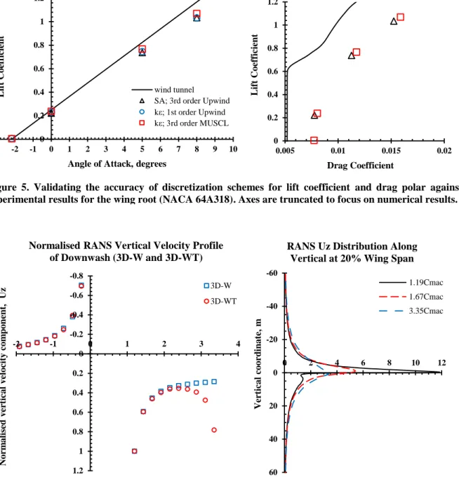
Preliminary parametric studies on the wing root section showed that both 2nd order upwind and 3rd order MUSCL
discretisation schemes with the one- and two-equation eddy-viscosity turbulence models (Spalart-Allmaras (SA) and compared with the Realisable k-ε, both treated with standard wall functions) provide results which are equally good and in agreement with the available wind tunnel data6 for prediction lift, but with a slight over-prediction for drag and
pitch,5 as seen in Fig. 5.
C. Spatial (Mesh) and Temporal Resolution
Empirical methods for calculation of the viscous wall unit (y+) are verified against a ‘first-cut’ simulation. All simulations were attempted at flight conditions (M = 0.23, ReMAC = 2.26 × 10⁷) and validated against available wind
tunnel data.6 Given the experimental setup is ambiguous, the assumption of standard sea-level conditions (𝜌
∞ = 1.225
kg/m3) are taken. Modelling of the geometry also excludes any possible experimental supports or probes, which
interferes with measured results.31
The wall shear stress 𝜏𝑤 within the inner region dominates the flow characteristics.32 The wall grid spacing is
determined empirically by friction velocity and the coefficient of friction for estimating wall shear stress with flow Reynolds Numbers > 109:33 𝜏𝑤= 1 2𝜌𝑉 2𝐶 𝑓 (7) Where; 𝐶𝑓 = [2 log10(𝑅𝑒) − 0.65]−2.3 (8)
This method for first-cell height estimation is then validated at against a ‘first-cut’ simulation with the y+ measured and averaged at increments of 0.25c across the aerofoil upper surface. This is found to be in good agreement (average y+ 4% smaller) with the wall shear stress relation for Newtonian fluids:32
𝜏𝑤= 𝜇 (
𝜕𝑢
𝜕𝑦)𝑦=0 (9)
Cases are then discretised with a body fitted grid of y+ = 30 at a growth rate of 1.2 up to 15 layers. Mesh sensitivity study is conducted by halving the element edge lengths in the mesh refinement region encompassing the wing and tail. Convergence is determined by observing for unchanging aerodynamic coefficients and vertical velocity component Uz. Halving the edge length in the refinement region results in a greatest of 2% change of Uz that is
measured just forward of the horizontal stabilizer at 25% tail span.
Elements in the refinement are almost cubic with a maximum cell aspect ratio of 1.09. The edge lengths in Table 1 are presented as an average and further expressed as a percentage of 𝐶𝑀𝐴𝐶.
The refinement zones for the mesh for the Fine case exceeded mesh counts and was unlikely to have brought significant gains. To utilize the Fine mesh for the time dependent case, the refinement regions were resized to refine 9 m span-wise from the wing root and extending downstream to encompass the entire horizontal stabilizer. This resizing was made after determining that the developing tip vortices has a negligible impact on the downwash for such a high wing aspect ratio. The Fine mesh is used for all cases.
Temporal scales are determined with the Courant-Friedrichs-Lewy condition:34
𝐶 =𝑈∞∆𝑡 ∆𝑥 ≤ 𝐶𝑚𝑎𝑥
(10) Table 1. Mesh sensitivity of vertical velocity Uz
Avg. cell edge length (% MAC) Peak Uz 3D-W Peak Uz 3D-WT Coarse 0.0746 m 1.79 % 3.43 m/s 5.01 m/s Medium 0.0377 m 0.9 % 3.45 m/s 4.91 m/s Fine 0.019 m 0.45% 3.49 m/s -
Where the edge length ∆𝑥 is taken from cubic elements in the refinement regions. A time step ∆𝑡 of 1e-4 s produces a Courant number of 0.41. The flow is given 1 s to develop which at this speed corresponds to approximately flow past 5 times the downwash domain length. This allows the flow to develop into a statistically steady state before sampling for time averaged results.
Figure 4. Body fitted grid [left] and refinement [right]. Results for downwash Uz taken along vertical white lines at every 1m increment from wing trailing edge to tail leading edge, 20% wing span from symmetry plane.
III.
Results and Discussion
The following are the results that compare the accuracy of the 1st & 2nd order Upwind, and 3rd order MUSCL
discretization schemes against the published wind tunnel data for the wing root section (NACA 64A318). It is determined that the 2nd and 3rd order schemes are equally accurate and only the most accurate results are shown in Fig.
5 for clarity.
Figure 5. Validating the accuracy of discretization schemes for lift coefficient and drag polar against experimental results for the wing root (NACA 64A318). Axes are truncated to focus on numerical results.
0 0.2 0.4 0.6 0.8 1 1.2 -3 -2 -1 0 1 2 3 4 5 6 7 8 9 10 Li ft Co efficie n t
Angle of Attack, degrees
Lift Curve comparison of Experimental and RANS CFD results
wind tunnel
SA; 3rd order Upwind kε; 1st order Upwind kε; 3rd order MUSCL 0 0.2 0.4 0.6 0.8 1 1.2 0.005 0.01 0.015 0.02 Lift Co efficie n t Drag Coefficient Drag Polar Comparison of Experimental and RANS CFD
Results
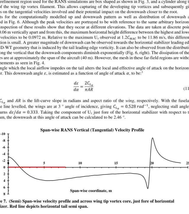
Figure 6. [Left] Pattern of up and downwash profile for the 3D-W and 3D-WT geometries. [Right] Distribution of UZ along vertical at 1.19CMAC (aft of wing), and 3.35CMAC (fore of tail).
-0.8 -0.6 -0.4 -0.2 0 0.2 0.4 0.6 0.8 1 1.2 -2 -1 0 1 2 3 4 No rm a li se d v er tica l v elo city c o m p o n en t, Uz
Normalised horizontal coordinate, X/CMAC Normalised RANS Vertical Velocity Profile
of Downwash (3D-W and 3D-WT) 3D-W 3D-WT -60 -40 -20 0 20 40 60 0 2 4 6 8 10 12 V er tica l co o rd in a te , m
Vertical velocity Uz, m/s RANS Uz Distribution Along
Vertical at 20% Wing Span
1.19Cmac 1.67Cmac 3.35Cmac
The refinement region used for the RANS simulations are box shaped as shown in Fig. 3, and a cylinder along the length of the wing tip vortex filament. This allows capturing of the developing tip vortices and subsequently give solutions on the tangential velocities involved and their potential impact on the downwash closer to the root.
Results for the computationally modelled up and downwash pattern as well as distribution of downwash are presented in Fig. 6. Although the peak velocities are portrayed to be with reference to the same arbitrary horizontal datum, inspection of these results show that they occur at different elevations. The data are taken at discrete points spaced 0.06 m vertically apart and from this, the maximum horizontal height difference between the highest and lowest vertical velocities to be 0.0972 m. Relative to the maximum Uz observed at 1.2𝐶𝑀𝐴𝐶 to be 11.86 m/s, this difference
in elevation is small. A greater magnitude of downwash can be observed towards the horizontal stabilizer leading edge for the 3D-WT geometry that is induced by the tail leading edge vorticity. It can also be observed from the distribution of Uz along the vertical that the downwash components diminish exponentially (Fig. 6, right). The dissipation of these
velocities are at approximately the span of the aircraft (40 m). However, the mesh in these far-field regions are without any refinements as seen in Fig. 4.
The angle which the local airflow impedes on the tail alters the local and effective angle of attack on the horizontal stabilizer. This downwash angle 𝜀, is estimated as a function of angle of attack 𝛼, to be:3
𝑑𝜀 𝑑𝛼=
2𝐶𝐿𝛼
𝜋𝐴𝑅 (11)
Where 𝐶𝐿𝛼 and 𝐴𝑅 is the lift-curve slope in radians and aspect ratio of the wing, respectively. With the fuselage
reference line levelled, the wings are at 3 ° angle of incidence, giving 𝐶𝐿𝛼= 0.528 𝑟𝑎𝑑
−1, neglecting stall angles.6
This returns 𝑑𝜀/𝑑𝛼 = 0.333. Taking the component of Uz just fore of the horizontal stabilizer with respect to the
freestream, the downwash at this angle of attack can be calculated to be 2.46 °.
In Fig. 7, the span-wise vertical velocity profile is shown at just fore of the horizontal stabilizer (red line depicts horizontal tail semi-span), plotted across the wing tip vortex core. It can be observed that velocities diminish exponentially beyond the core radius at < 18 m wing span. These velocities diminish at the mid-span due to the wing’s large aspect ratio. This helps determine that the vertical tangential velocities has a negligible impact on the downwash region towards the tail. The change in values observed towards the root are caused by the deflection of airflow around the leading edge of the stabilizer. The midsection of the tail is supposed to be masked by the fuselage/empennage section but however, is modelled here.
The vortex core radius measured at 3.35𝐶𝑀𝐴𝐶 (plane at tail leading edge) is in agreement with typical values,14
where the radii, defined as the distance from the vortex core to the point of maximum tangential velocity is in the order of 1% wing span (Fig. 9). The characteristic tangential velocity profile is also observed. However, when comparing the results to three idealized models of trailing wake vortices,15 results differ. The estimation of the vortex
strength by initial circulation Γ0, for the calculation of tangential velocities with the idealized models is given by:
Figure 7. (Semi) Span-wise velocity profile and across wing tip vortex core, just fore of horizontal stabilizer. Red line depicts horizontal tail semi span.
-10 -8 -6 -4 -2 0 2 4 6 8 0 5 10 15 20 25 V er tica l (ta n g en tia l) v elo city , m /s Span-wise coordinate, m
Where 𝑀𝑔 is the weight of the aircraft. However, this is best approximated with the aircraft in equilibrium, and the results under which the conditions are taken may not be in cruise although flight Reynolds numbers are simulated.35
The vortex core size from the results here are very likely to be still developing, as they are taken along the plane in the downwash regions. It can be seen in Fig. 8 that the vortex core diameter is small - but with high intensity by judging from the tangential velocities in Fig. 7 - relative to the span of downwash.
As RANS solutions are able to only resolve for the mean variables of the flow field by Reynolds decomposition, transient analyses are required to provide further insight to this profile and on any unsteadiness to these results. These datasets are time-averaged to provide their mean and fluctuating values - represented as a standard deviations - of velocities across the same sampled locations used in RANS. Only the 3D-WT model and mesh was used for the transient case.
DDES solutions are conducted at the inboard section of the wing root only (Fig. 3). For these analyses, the flow referencing the freestream, is given 1 s to develop. This corresponds to approximately 5 times the flow past the
chord-Γ0=
𝑀𝑔 𝜋
4𝜌𝑏𝑈∞ (12)
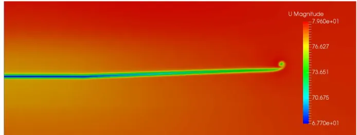
Figure 8. Span-wise velocity magnitude contour along plane at 1.6CMAC
Figure 9. [Left] Close-up of wingtip vortex. [Right] Vertical velocity UZ contour. Embedded scale depicts 1.00 m.
at every 50 time steps where ∆𝑡 =1e-4 s and time-averaged. This amounts to 5000 time samples. Within the initial 0.1 s, an initial vortex roll up36 can be observed trailing the wings (Fig. 11).
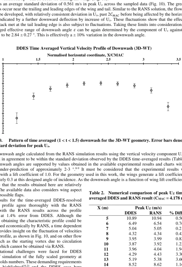
There is an average standard deviation of 0.561 m/s in peak Uz across the sampled data (Fig. 10). The greatest
fluctuations occur near the trailing and leading edges of the wing and tail. Similar to the RANS solution, the flow can be seen to be developed, with relatively consistent deviation in Uz, past 2𝐶𝑀𝐴𝐶 before being affected by the horizontal
stabilizer indicated by a further downward deflection by increase of Uz. These fluctuations show that the effective
angle of attack met at the tail leading edge is also subject to fluctuations. Taking these limits into consideration, the time-averaged effective range of downwash angle 𝜀 can be again determined by the component of Uz against the
freestream, to be 2.84 ± 0.27 °. This is effectively a ± 10% variation in the downwash angle.
The downwash angle calculated from the RANS simulation results using the vertical velocity component Uz are
similar and in agreement to be within the standard deviation observed by the DDES time-averaged results (Table 2). These downwash angles are supported by values obtained in the available experimental results and charts with an expected under-prediction of approximately 2-3 °.8-9 It must be considered that the experimental results were
conducted with a lift coefficient of 1.0. For the geometry used in this work, the wings generate a lift coefficient of approximately 0.3 at this designed angle of incidence. As the downwash angle is a function of wing lift coefficient, it is arguable that the results obtained here are relatively
accurate. The available data also considers wing aspect ratios and possible flaps.
The results for the time-averaged DDES-resolved downwash profile agree thoroughly with the RANS solution, with the RANS results across the profile averaging at 1.4% error from DDES. Although the purpose of obtaining the characteristic profile could be accomplished economically by RANS, a time dependent solution provides insight on the fluctuation of velocities across the profile, as shown in Fig. 10, and on other flow features such as the starting vortex due to circulation (Fig. 11), which cannot be obtained via RANS.
Computational challenges were faced for DDES because of simulation of the fully scaled geometry at flight Reynolds numbers. These demanding requirements have been highlighted19,21 and the DDES case here
utilizes 90 million elements with just the refinement box
Figure 10. Pattern of time averaged (1 < t < 1.5) downwash for the 3D-WT geometry. Error bars denote the standard deviation for peak Uz.
0 2 4 6 8 10 12 14 1 1.5 2 2.5 3 3.5 V er tica l v elo city c o m p o n e n t, Uz , m /s
Normalised horizontal coordinate, X/CMAC
DDES Time Averaged Vertical Velocity Profile of Downwash (3D-WT)
Table 2. Numerical comparison of peak UZ time-averaged DDES and RANS result (CMAC = 4.178 m)
X (m) Peak UZ (m/s)
DDES RANS % Diff.
5 10.89 10.94 0.50 6 6.49 6.54 0.76 7 5.04 5.05 0.21 8 4.32 4.34 0.42 9 3.95 3.99 0.83 10 3.87 3.92 1.23 11 3.96 4.04 1.94 12 4.29 4.43 3.30 13 5.19 5.38 3.60 14 8.52 8.62 1.16 Avg. - - 1.40
capturing part of the downwash. At these spatial and temporal scales, approximately 9 days of computational time and 1 TB of data are used just for the transient case.
The meshing techniques used can be improved. Having a box-shaped enclosure to define mesh refinement as seen in Fig. 4 unnecessarily inflates the amount of elements in regions unrequired to capture the thin vortex sheet trailing the wings, especially at such a benign angle of attack. By optimizing the mesh, the turbulent scales involved could have been better resolved.
IV.
Outlook
While validating the geometry against experimental data an over-prediction of drag is observed. This is attributed to the use of wall functions interfering with the modelling of shear layers.37 For flows over a curved surface such as
an airfoil, this requires capturing of near wall features such as a resolved boundary layer and any reversed flows due to adverse pressure gradients. However, for the context of wake studies, capturing the boundary layer may be of less significance. This is where hybrid methods like DES prevails. As vortex shedding involves the physical detachment of flow from the body, the modelling of the shedding of turbulent structures from the boundary layer or near wall region and transition into wake would have to be considered. This encourages further studies on the impact of DES and its RANS-modelled wall regions against full LES methods on downstream wakes. This is important in the context of modelling of aerodynamic interactions. It would be useful to advance the understanding and implications of applying DES and as compared to LES models for the purposes wake studies.
Conceptually, the wing in such a context is a vortex generator. Therefore, for further extending this study into one which provides insight on the effectiveness of a horizontal stabilizer within a turbulent wake, the wings in this case may be replaced by an upstream vortex generator of a much simplified geometry. This is analogous to studies conducted on the assessment of aerodynamic bodies within turbulence.
Acknowledgments
This work is supported by our partners at AviationLearn (www.aviationlearn.com) through the Industrial Postgraduate Program. The workstation that runs a pair of Intel Xeon E5-2695v4 (18 cores) with 256 GB of RAM is gratefully acknowledged. The guidance from staff at both the University of Glasgow Singapore and Singapore Institute of Technology is also appreciated.
References
1B. Etkin, Dynamics of Atmospheric Flight, Dover Publications, 1972.
2B. Etkin and L. D. Reid, "Chapter 2: Static Stability and Control - Part I," in Dynamics of Flight, Wiley, 1994, pp. 18-33.
3R. C. Nelson, "2.3 Static Stability and Control," in Flight Stability and Automatic Control, WCB/McGraw-Hill, 1998, pp.
47-52.
4W. F. Philips, "Chapter 4: Longitudinal Static Stability and Trim," in Mechanics of Flight, Wiley, 2010, pp. 384-391.
5K. J. B. Tan and P. C. Wang, "Computational Modelling and Aerodynamic Analysis of a Conventional Fixed-Wing Aircraft,"
in Advances in Simulation: The Future of Flight Simulation, London, 2016.
6"Aerodynamic Data for Structural Loads: C-130," Lockheed, California, 1953.
Figure 11. Instantaneous chord-wise velocity magnitude and vorticity contours of starting vortex rollup leaving the wing at t = 0.05 s. Peak contours show velocity = 97.5 m/s and vorticity = 1223 s-1
7J. J. D. Anderson, "Chapter 5: Incompressible Flow over Finite Wings," in Fundamentals of Aerdynamics, New York,
McGraw-Hill, 2001, pp. 412-484.
8A. Silverstein and S. Katzopf, "Design Charts for Predicting Downwash Angles and Wake Characteristics Behind Plain and
Flapped Wings," NACA, 1939.
9A. Silverstein, S. Katzopf and W. K. Bullivant, "Downwash and Wake Behind Plain and Flapped Airfoils," NACA, 1939.
10J. D. Anderson, Jr., "Chapter 2: Aerodynamics of the Airplane: The Drag Polar," in Aircraft Performance and Design,
McGraw-Hill Book Co.-Singapore, 1999, pp. 103-105.
11C. Paek, J. Chung and R. Czerwiec, "C-130 Aerodynamic Loads Assessment for the USN/USMC Part I: P-3C CFD
Verification," in 47th AIAA Aerospace Sciences Meeting Including The New Horizons Forum and Aerospace Exposition, Orlando, Florida, 2009.
12J. Chung, C. Paek and R. Czerwiec, "C-130 Aerodynamic Loads Assessment for the USN/USMC Part II: C-130 Analysis,"
in 47th AIAA Aerospace Sciences Meeting Including The New Horizons Forum and Aerospace Exposition, Orlando, Florida, 2009.
13M. Ghoreyshi and R. M. Cummings, "From Spreadsheets to Simulation-Based Aircraft Conceptual Design," Applied Physics
Research, vol. 6, no. 3, 2014.
14F. H. Proctor, "Numerical Simulation of Wake Vortices Measured During the Idaho Falls and Memphis Field Programs," in
14th AIAA Applied Aerodynamic Conference, New Orleans, Louisiana, 1996.
15D. P. Delisi, G. C. Greene, R. E. Robins, D. C. Vicroy and F. Y. Wang, "Aircraft Wake Vortex Core Size Measurements," in
21st AIAA Applied Aerodynamics Conference, Orlando, FL, 2003.
16N. N. Ahmad, F. H. Proctor, F. M. L. Duparcmeur and D. Jacob, "Review of Idealized Aircraft Wake Vortex Models," in
AIAA SciTech, National Harbor, Maryland, 2014.
17F. T. Johnson and E. N. Tinoco, "Thirty Years of Development and Application of CFD at Boeing Commercial Airplanes,
Seattle, Washington," American Institute of Aeronautics and Astronautics, 2005.
18M. R. Hall, R. T. Biedron, D. N. Ball, D. R. Bogue, J. Chung, B. E. Green, M. J. Grismer, G. P. Brooks and J. R. Chambers,
"Computational Methods for Stability and Control (COMSAC): The Time Has Come," American Institute of Aeronautics and Astronautics, 2004.
19S. A. Morton, J. R. Forsythe, K. D. Squires and R. M. Cummings, "Detached-Eddy Simulations of Full Aircraft Experiencing
Massively Separated Flows," in The 5th Asian Computational Fluid Dynamics Conference, Busan, Korea, 2003.
20D. Drikakis, D. Kwak and C. C. Kiris, "Computational Aerodynamics: Advances and Challenges," The Aeronautical Journal,
vol. 120, no. 1223, pp. 13-36, 2016.
21P. R. Spalart and V. Venkatakrishnan, "On the Role and Challenges of CFD in the Aerospace Industry," The Aeronautical
Journal, vol. 120, no. 1223, pp. 209-231, 2016.
22P. R. Spalart, W.-H. Jou, M. Strelets and S. R. Allmaras, "Comments on the Feasibility of LES for Wings, and on a Hybrid
RANS/LES Approach," in Advances in DNS/LES, 1997.
23P. R. Spalart, S. Deck, M. L. Shur, K. D. Squires, M. K. Strelets and A. Travin, "A New Version of Detached-Eddy
Simulation, Resistant to Ambiguous Grid Densities," Theoretical and Computational Fluid Dynamics, pp. 181-195, 2006.
24P. R. Spalart, "Young-Person's Guide to Detached-Eddy Simulation Grids," NASA Langley Research Center, Virginia, 2001.
25J. R. Forsythe, K. D. Squires, K. E. Wurtzler and P. R. Spalart, "Detached-Eddy Simulation of the F-15E at High Alpha,"
Journal of Aircraft, vol. 41, no. 2, 2004.
26Customer Training Systems Department, "Volume I: General Aircraft," in C-130H-30 Hercules Traning Manual, Lockheed
Aeronautical Systems Company - Georgia, 1993, pp. 2-5.
27P. R. Spalart and S. R. Allmaras, "A One-Equation Turbulence Model for Aerodynamic Flows," in AIAA 30th Aerospace
Sciences Meeting and Exhibit, Reno, NV, 1993.
28C. L. Rumsey, "Apparent Transition Behavior of Widely-Used Turbulence Models," Apparent Transition Behavior of
Widely-Used Turbulence Models, vol. 28, pp. 1460-1471, 2007.
29C. L. Rumsey, D. O. Allison, R. T. Biedron, P. G. Buning, T. G. Gainer, J. H. Morrison, S. M. Rivers, S. J. Mysko and D. P.
Witkowski, "CFD Sensitivity Analysis of a Modern Civil Transport Near Buffet-Onset Conditons," NASA/TM-2001-211263, 2001.
30NASA Langley Research Center, "Turbulence Modeling Resource," NASA, 2016. [Online]. Available:
https://turbmodels.larc.nasa.gov/spalart.html. [Accessed March 2017].
31J. H. Ferziger and P. M., Computational Methods for Fluid Dynamics, Springer-Verlag, 2001.
32C. M. Fremaux and R. . M. Hall, "(Compilation) COMSAC: Computational Methods for Stability and Control," Virginia,
2004.
33P. C. Wang, "Large Eddy Simulation of High Speed Convergent-Divergent Nozzle Flows, PhD Thesis," Loughborough
University, 2012.
34H. Schlichting, Boundary Layer Theory, McGraw-Hill Science/Engineering/Math, 1979.
35R. Courant, K. Friedrichs and H. Lewy, "On the Partial Difference Equations of Mathematical Physics," AEC Research and
Development Report, NYO-7689, New York: AEC Computing and Applied Mathematics Centre, New York, 2008.
36F. Holzapfel, "Aircraft Wake Vortex Evolotuion and Prediction," 2005.
37J. D. Anderson, Jr., "Chapter 4: Incompressible Flow Over Airfoils," in Fundamentals of Aerodynamics, New York,
38E. N. Tinoco, O. P. Brodersen, S. Keye, K. R. Laflin, E. Feltrop, J. C. Vassberg, M. Mani, B. Rider, R. A. Wahls, J. H.
Morrison, D. Hue, M. Gariepy, C. J. Roy, D. J. Mavriplis and M. Murayama, "Summary of Data from the Sixth AIAA CFD Drag Prediction Workshop: CRM Cases 2 to 5," in Drag Prediction Workshop, 2016.
![Figure 4. Body fitted grid [left] and refinement [right]. Results for downwash U z taken along vertical white lines at every 1m increment from wing trailing edge to tail leading edge, 20% wing span from symmetry plane](https://thumb-us.123doks.com/thumbv2/123dok_us/1877440.2774081/7.918.127.798.149.753/figure-refinement-results-downwash-vertical-increment-trailing-symmetry.webp)