Bard Digital Commons
Bard Digital Commons
Senior Projects Spring 2019 Bard Undergraduate Senior Projects
Spring 2019
Self-Driving Cars: Exploring the Potential of Using Convolutional
Self-Driving Cars: Exploring the Potential of Using Convolutional
Neural Network to Overcome Road Variation
Neural Network to Overcome Road Variation
Shida Wang
Bard College, [email protected]
Follow this and additional works at: https://digitalcommons.bard.edu/senproj_s2019
Part of the Artificial Intelligence and Robotics Commons
This work is licensed under a Creative Commons Attribution-Noncommercial-No Derivative Works 4.0 License.
Recommended Citation Recommended Citation
Wang, Shida, "Self-Driving Cars: Exploring the Potential of Using Convolutional Neural Network to Overcome Road Variation" (2019). Senior Projects Spring 2019. 136.
https://digitalcommons.bard.edu/senproj_s2019/136
This Open Access work is protected by copyright and/or related rights. It has been provided to you by Bard College's Stevenson Library with permission from the rights-holder(s). You are free to use this work in any way that is permitted by the copyright and related rights. For other uses you need to obtain permission from the rights-holder(s) directly, unless additional rights are indicated by a Creative Commons license in the record and/or on the work itself. For more information, please contact
Self-Driving Cars: Exploring the Potential of Using Convolutional Neural Network to Overcome Road Variation
Senior Project Submitted to
The Division of Science, Mathematics, and Computing of Bard College
by Shida Wang
Annandale-on-Hudson, New York May 2019
Thank you to Professor Sven Anderson for advising me through the whole year. Also thank you to Vivian Han for staying with me through highs and lows and helping me with writing. And to my close friend in these four years, Xishixin Song for getting me through this semester.
1. Introduction ...1 1.1 Purpose ...5 1.2 Scope ...6 2. Background ...7 2.1 Neural Network ...7 2.1.1 Neuron ...8 2.1.2 Activation Function ...9 2.1.3 Training ...9 2.1.4 Overfitting ...10 2.1.5 Early Stopping ...10
2.2 Convolutional Neural Network ...11
2.2.1 Filters ...12 2.3 Proportional-Integral-Derivative Controller ...13 2.3.1 Proportional Control ...13 2.3.2 Integral Control...14 2.3.3 Derivative Control ...14 2.4 Unity ...15 2.5 Keras ...15 3. Methods ...16 3.1 Network Structure...16 3.2 Road ...17 3.3 Vehicle ...18
3.4 Data Collecting and Training ...19
3.5 Steering Angle ...19
3.6 Deviation Distance ...20
4. Results and Analysis ...21
4.1 Chosen Model ...21
4.2 Testing Track ...22
4.3 Track Completeness ...23
4.3.3 CNN’s Performance on Road with Missing Edges ...24
4.4 Steering Angle ...25
4.5 Deviation Distance ...27
The use of self-driving cars can benefit the society in many ways, such as reducing traffic accidents and enabling disabled people to travel independently. The potential of reducing traffic accidents can be considered most important, since in 2017, mistakes made by human drivers were the cause of over 90% of the traffic accidents, leading to 40,100 people’s deaths in the United States. If human drivers were replaced by autonomous systems, the number of traffic accidents would decrease. Although the concept of self-driving car was raised since at least the 1920s, a commonly accepted development of self-driving car has not yet appeared. A significant challenge is the creation of a system that can accurately detect the environment around itself and then form the right driving command. Recent progress in deep learning suggested that
convolutional neural networks are a form of machine learning that can be trained to extract features and use those features to control a car. This project focuses on extending the network model in the paper published by NVIDA in 2016 [1]. The aim of the project is to evaluate how well a convolutional neural network could perform on a simple, simulated roadway with road varying and missing road edges.
1 Introduction
A self-driving car, also known as an autonomous car, is a vehicle that is able to sense the environment around it and move from the start point to the destination with no human input. Since the most significant difference between a self-driving car and a normal car is that a self-driving car does not need human while driving, it could decrease the number of traffic accidents caused by human drivers’ mistakes. Human drivers’ mistakes can be generally split into two groups. One of these is active
mistakes, such as when a driver is trying to drink coffee while driving; he may be not fully paying attention to driving and made a careless decision leading to a traffic accident. The other one is passive mistakes: for example, something not expected suddenly happens in front of a car and the driver does not have enough time to make the optimal decision to deal with the situation and thus makes a mistake. With self-driving cars, the active mistakes may be avoided completely, since the only thing the cars focus on is driving safely. Passive mistakes may be reduced by creating systems that respond faster and more reliably than humans.
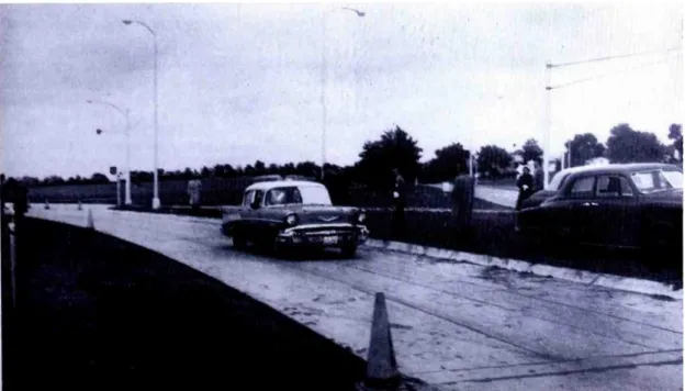
The concept of self-driving car was raised since at least the 1920s, before computers became widely used. Therefore, people built self-driving cars with infrastructure navigating the cars. One of those developments was the RCA’s
experimental detector circuits buried in the pavement and the lights along the edge of the road were used to send signals to the RCA special radio receivers and visual devices equipped in the test car. These devices then transformed those signals to driving commends and guide the car. The test showed ultimate possibilities of the automatic electric highway; however, the huge cost of building that highway limited its application for public use. Also, the experiment did not include anything other than cars (e.g. traffic lights) and it was proven that the system was stable only when the car was driving in low speed. This system was not intelligent enough to drive the car in a real-world situation.
Figure 1: RCA’s automatic electronic highway experiment
By the 1960s, artificial intelligence researchers began dreaming of cars smart enough to navigate on their own. The goal essentially changed to reverse-engineer the relevant systems in a moving animal: sensing, processing and reacting [3]. Then, after
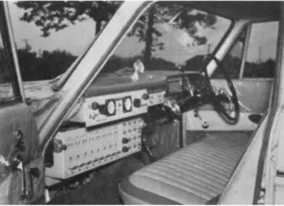
the digital revolution, the digital computer became able to make this goal come true. The first truly automated car in the world was developed by Japan’s Tsukuba
Mechanical Engineering Laboratory in 1977 [4] (Figure 2). This vehicle carried two cameras and used analog computer technology for signal processing. It tracked white street markings on a dedicated circuit and could drive up to 20 miles per hour. This development marked the beginning of the new era of achieving self-driving cars. Since then, many automobile giants started taking efforts to build autonomous vehicles.
Figure 2: Tsukuba Mechanical Engineering Laboratory’s self-driving car.
In 2004, the Defense Advanced Research Projects Agency (DARPA) held the DARPA Grand Challenge 2004 to accelerate the development of autonomous vehicle technologies that can be applied to military requirements. The goal was to build an autonomous car to run a 142-mile course across the Mojave Desert from Barstow, California to Primm, Nevada. No team was able to complete the difficult task. Then,
in 2005, when the same challenge was raised again, the Stanford Racing Team won the competition with 5 out of 195 teams completed the task. In 2007, the DARPA Grand Challenge shifted its focus to urban city traffic. In all 11 vehicles, 6 of them succeeded in finishing a 60-mile urban course in moving traffic in less than 6 hours [5][6]. The most significant advance was in the ability of a car to detect useful features around it. Most of the competitors participating the DARPA Challenge went through this part with different ways of implementing their own feature extractors.
Convolutional neural networks (CNN) are a wise solution to the challenge of computer vision due to its ability to find out the most important features from the training data through feature extraction. Thus, it should also help with building self-driving cars. CNN was first used in building self-self-driving cars by Pomerleaus
Autonomous Land Vehicles in Neural Networks (ALVINN) in 1989. A car steered by CNN ran at a speed of 19 miles per hour. Since then, more and more people started to use CNN in building self-driving cars. Today, companies like Google, Tesla and NVIDA are all using deep neural network for environment detection as a part of their autonomous vehicles. This project focuses on extending the network model in the paper published by NVIDA in 2016[1]. This project explores the possibility of using a single output convolutional neural network to drive a car on the road with missing road edges in a simulated environment.
1.1 Purpose
This project focuses on developing a self-driving car with convolutional neural networks. The network model used in this project is inspired from NVIDA’s published paper [1]. There are two goals in this project:
1. Compare the performance of a convolutional neural network driving the car on road with road edges and the performance of a proportional-integral-derivative (PID) controller driving the car on road with road edges.
2. Compare the performance of a convolutional neural network driving on a simulated road with road edges and the performance of the same convolutional neural network driving on a simulated road with partly missing road edges.
The first comparison aims to find out if CNN is a better solution to driving a car on a simple road than PID controller. A proportional-integral-derivative controller is a control method used in industrial control. Since the PID controller does not learn anything from examples, using a PID controller to control the car can be seen as a method that predates machine learning. As opposed to PID controller, a CNN could learn from training examples to form better solutions to tasks. Therefore, using a well-trained CNN to drive the car may give a better performance than using a PID
The second goal of this project explores the capacity of CNN encountering a real-world situation that the road edges suddenly disappear while driving. Since road edges could be important features for a CNN to form accurate driving commands, missing road edges may affect the performance of CNN.
1.2 Scope
This whole project is simulated in Unity, not in the real world, therefore, there are limitations:
1. The simulated car is only able to predict the steering angle. It should not be considered fully autonomous.
2. The physics of driving the car in this project cannot fully simulate driving a car in the real world.
3. Road variables other than turning and missing road edges are not simulated in this project.
2 Background
This chapter includes the information needed for this project. Convolutional neural network, proportional-integral-derivative control and Unity simulator are introduced here.
2.1 Neural Network
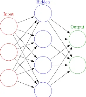
A neural network is a computational learning system that transforms input data to desired output through a network of functions [7]. The concept of neural network was first inspired by biological neural networks. A neural network contains a collection of connections of nodes called artificial neurons. Through training, a neural network is able to form outputs to finish a given task. Inputs become desired outputs by getting calculated in neurons while passing through connected neurons. Figure 3 is an example of a neural network consist of 3 input units, 2 output units and a hidden layer.
Figure 3: A neural network with 3 input units, 2 output units and a hidden layer
2.1.1 Neuron
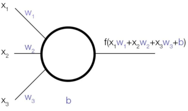
Neurons are elementary units in neural networks. Each neuron has its own weight which is initialized with a random number and then changed during training process. After training, when a neuron receives inputs, it first sums up the weighted inputs and then adds a bias to the sum. Figure 4 shows the calculation in a neuron with three inputs.
Figure 4: Calculation in a neuron with three inputs is shown here. In this figure, x are the inputs, w are the weights for each value, b represents the bias term. The sum of weighted inputs and bias is calculated and transformed by the function to the output.
2.1.2 Activation Function
Activation function determines if a neuron should fire or not based on the summed value of weighted inputs and bias. The activation function used in this project is rectified linear unit function. The rectified linear unit function only allows a neuron to send its output to other neurons connected to that neuron if the output is greater than 0. Otherwise, 0 is sent to the connected neurons.
2.1.3 Training
Once a neural network has been structured for a particular application, that network needs to be trained in order to output the desired output values. During the training process, example inputs are provided to the network. The network generates the
output with its current weight and then calculates the error between the output value and the desired output value in the training example. Then, propagating in the reverse direction from output layer to input layer, each weight is changed due to its portion contribution to the error. This process occurs over and over as the weights are changed to reduce the error. In this project, the function for calculating error is mean squared error (MSE) formula. It is chosen since its differentiable and also with the square sign, positive errors and negative errors will not cancel out each other. In this formula shown below, n is the number of training examples, f(X) is the actual output value and Y is the desired output value.
2.1.4 Overfitting
When the error value reaches its minimum, the training process stops. However, a neural network with smallest error does not guarantee the best performance when testing since it may overfit the data. An overfitted model is a model that contains more parameters than can be justified by the data. In other words, this model more perfectly fits the training data but gives a poor performance on testing data
2.1.5 Early Stopping
One of the ways to prevent overfitting is to take a part of training examples out to be a validation set. As the validation data is independent of the training data, a network’s performance on the validation data is a good measure of training process [8]. During
the training process, when the error value for validation set stops decreasing, stopping the training process produces a model that better fits the testing data – a more general model. In Figure 5, t represents the time when the training process should be stopped.
Figure 5: The value t indicates the time to stop the training process [8].
2.2 Convolutional Neural Networks (CNN)
Convolutional neural networks(CNN) are a type of neural network that has proven very effective in areas such as image recognition and classification. CNN was first introduced by Lecun in 1998 to classify hand written digits in a 32x32 image [9]. The advantage of using a CNN to deal with image processing is that a CNN can vastly reduce the number of parameters in the network by applying filters. In other words, a CNN learns useful features in an image faster than a usual neural network. Since in this project the only input to the network model is an image, using a CNN is an effective solution.
2.2.1 Filters
The word convolutional in convolutional neural network describes how the input image of the network is modified by a filter. The filter slices left to right across the image from top to bottom to form a convolved output as shown in Figure 6. Figure 6 shows how a 2x2 filter modifies a 5x5 input image and forms the convolved output. In the formula given, c is the filter’s output, n stands number of rows, m stands for number of columns, I represents the value of the input image and F is filter’s value. The sums of the products of each pair of image value and filter value together generate the convolved output.
Figure 6: A filter modifying an input image to a convolved output by calculating the sum of the products of the corresponding values in the input image and the filter.
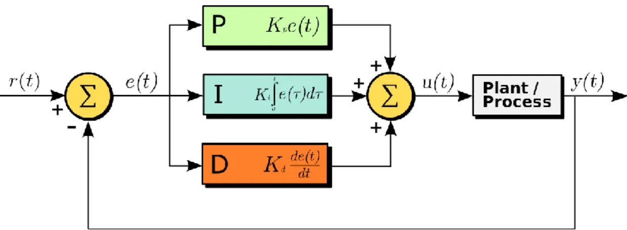
2.3 Proportional–Integral–Derivative (PID) Controller
A proportional–integral–derivative controller is a control loop feedback mechanism widely used in industrial control systems and a variety of other applications requiring continuously modulated control. A PID controller continuously calculates an error value as the difference between a desired setpoint (SP) and a measured process variable (PV) and applies a correction based on proportional, integral, and derivative terms (denoted P, I, and D respectively) which give the controller its name. The difference between the desired output and actual output is called cross-track error (CTE). In this project, Kp and Kd were set to 10, and Ki was set to 1.
Figure 7: The PID controller takes an input and produce its output
r(t) = SP e(t) = CTE u(t) = change y(t) = output K = gain factor
2.3.1 Proportional Control
P as the component that is proportional to the CTE, which is SP − PV = e(t). In this project, it has a direct impact on the car’s path because it makes the car “correct” in
proportion to the error in the opposite direction. For example, if the error value is large and positive, by applying gain factor K, the control output will also be
proportionately large and positive. There is a natural overturning effect that will cause the car to swing left and right eventually driving the car off-track while only using proportional control. Larger values of P will cause the car to oscillate faster.
2.3.2 Integral Control
A way to cancel the overturning is to add integral control. Term I considers the past value of the CTE and it is measured by the integral of the CTE over time. The reason we need it is that there is likely residual error after applying the proportional control. Error in proportional control ends up causing a bias over a period of time that
prevents the car stay in the center. This integral term seeks to eliminate this residual error by adding a historic cumulative value of the error.
2.3.3 Derivative Control
Term D is the best estimate of the next round’s error in the future, based on its current rate of change. When the car has turned enough to reduce the cross-track error, D will inform the controller that the error has already declined. As the error becomes smaller over time, the counter steering won’t be as sharp helping the converge the movement to the target trajectory.
2.4 Unity
Unity is a cross-platform real-time engine developed by Unity Technologies. It was first announced and released in June 2005 at Apple Inc.'s Worldwide Developers Conference as an OS X-exclusive game engine [10]. The primary programming language used in this engine is C#. Unity can be used to create three-dimensional games as well as simulations for the real world. This project uses the Unity engine in order to obviate the time and money cost by implementing roads, cars and
experiments in the real world.
2.5 Keras
The convolutional neural network used in this project is implemented with Keras. Keras is an open-source neural-network library written in Python. It was developed as a part of the research effort of project ONEIROS (Open-ended Neuro-Electronic Intelligent Robot Operating System) [10]. Implemented with many commonly used elements of building neural networks such as layers and activation functions, Keras was designed to enable fast experimentation with neural networks. In addition to standard neural networks, Keras has support for convolutional and recurrent neural networks.
3 Methods
This chapter includes how the neural network is trained.
3.1 Network structure
Figure 8 shows the structure of the neural network used in this project. From the bottom to the top, there are a normalization layer, 5 convolutional layers and 3 fully connected layers. Normalization layer is used to accelerate GPU processing. The convolutional layers perform feature extraction, which chooses useful features. In the first 3 convolutional layers, the filter size was set to 5x5 with a 2x2 stride. The forth convolutional layer has a filter size was set to 3x3 with a 2x2 stride. In the last
convolutional layer, the filter size was still 3x3 but the stride was changed to 1x1. The fully connected layers are designed to function as a controller for steering. They give out the output control value. The input for this model is the pictures taken of the road. The output of this single output model can be any number between -1 and 1 and used as the steering command for the self-driving car.
Figure 8: Network model used in this project
3.2 Road
The road simulated in this project is a two-way road with two white line on its sides representing the load edges and a yellow line splitting the two lanes. Each lane is 3.5m in width. The car drives on the right lane, following the traffic rules. The road is composed of 2-meter segments and each segment is randomized to have an angle in the range from 90 to -90. However, the turnings are limited by
minimum turning radius. This road’s minimum turning radius is set to 6m,
according to the road construction standard used in China. When the CNN is tested on road with missing road edges, each road edge on the side of the road randomly disappears with a probability of 0.05. The length of the missing road edges is also randomized between 2m to 10m with a standard normal distribution. There is no road variation such as signs and other cars simulated in this project. The only two types of variation involved in this project are turning and accidentally missing road edges. Figure 9 is an above view of a part of the road.
Figure 9: An aerial view of the road. The upper and lower lines are the road edges in white color. The line in the middle is a yellow line.
3.3 Vehicle
The size of the vehicle simulated in this project has a length of 3m and a width of 1.8m, which matches the size of a small car. The vehicle is designed as a two-wheel drive car with only two front wheels that can turn to simulate the most common car existing in real world. A camera is located in the front of the vehicle. During data collecting processes, the camera keeps taking pictures with the speed of 30fps. The
images are stored in the size of 160x120 pixels. During testing, the camera also continuously takes pictures at 30fps for CNN to navigate the car. The speed of the car was set to 18 miles per hour. Figure 10 shows a sample image taken by the camera while the car is driving on the road.
Figure 10: Sample images taken by the camera while the car is driving on the road.
3.4 Data Collecting and Training
In this project, all data were collected in Unity simulator. The car was driven by PID controller during data collecting process. A total of 100000 images were collected while the car was driving on the road with complete road edges. Then, 50000 images were collected while the car was driving on the road with incomplete road edges. When the loss of validation data continuously increases for 5 epochs, the training process stopped. For each training session, the model took about 4 hours to train. The model was given 10 training sessions beginning from random initial conditions and the model with least error value was chosen to be tested.
3.5 Steering Angle
In a real-world approach, driving a car with less unnecessary steering makes it better and safer. Therefore, steering angles are important data for judging whether a driving method is good or not. When evaluating the steering angles of the performances, both
the PID controller and the CNN model were tested on different sets of data other than the training dataset and the validation dataset. The variances of steering angles were calculated in order to compare the smoothness of driving by the following formula:
In this formula, s² stands for variance, M is the mean of the steering angles, x is the actual steering angle and n is the number of steering angles.
3.6 Deviation Distance
With steering angles, only the smoothness of driving can be evaluated but the ability of a method to keep the car on the center line is not known yet. Therefore, evaluating the deviation distance from the car to the center line is also necessary to evaluate a driving method. The means of deviation distances are used here to compare the performances of different driving methods.
4 Results and Analysis
After the network model was trained, it was tested on 5 different tracks. This chapter includes the results and data analysis.
4.1 Chosen Model
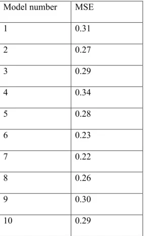
In all 10 trained models, the model with least error value, 0.22, was chosen for testing. Error values fell in between 0.34 and 0.22. The average error value for 10 models was 0.279. Table 1 shows the error values of each model. Figure 11 demonstrates the distribution of the error values.
Model number MSE
1 0.31 2 0.27 3 0.29 4 0.34 5 0.28 6 0.23 7 0.22 8 0.26 9 0.30 10 0.29
Figure 11: Box plot of the error values. The maximum was 0.34 and the minimum was 0.22. The median was 0.285.
4.2 Testing Track
5 different Tracks were generated in Unity engine for testing the network model. They are each 2km in length. Figure 12 shows all the tracks. Tracks 1 to 5 are listed in the order from top to bottom, left to right. The red point at one end of each track is the car’s start point.
Figure 12: Test tracks 1 to 5. Each track is 2km in length. In all 5 tracks, there are approximately 3.7km nearly straight road; the remaining 6.3km are all turnings.
4.3 Track Completeness
Successfully driving the car through the test tracks is the most obvious indication that a driving method is able to handle that track.
4.3.1 PID Controller’s performance
With the help of the low speed limitation, the PID controller was guaranteed to have enough time to drive the car towards the further side before driving the car off the road. Also, since the PID controller knew the distance between the car and the center of the lane and did not form decisions based on road edges, missing road edges did not affect its performance.
4.3.2 CNN’s Performance on Road with Edges
The CNN model completed 8.41km out of 10km in total while driving on the road with edges. It was able to navigate the car through track 1, 2, 4 and 5 but failed to complete track 3. The car went off the road when the road was crossing itself [Figure 13]. This failure showed that the CNN model could possibly get confused by
crossings. Training the model with more road crossing examples may help eliminate this kind of failure.
Figure 13: The place the car went off the road
4.3.3 CNN’s Performance on Road with Missing Edges
While driving the car on road with missing edges, the model completed 5.29km out of 10km with only completing track 2 and 5. In all other 3 tracks, the car completed part of the road with straight line and some turnings and then went off when the road edges disappeared at relatively sharp turnings. Also, knowing that track 2 and 5 had the smallest ratios of turnings among all 5 tracks, a conclusion maybe drawn that the CNN model could not handle all cases of missing road edges. Figure 14 points out the places where the car went off the road.
Figure 14: The place the car went off the road
4.4 Steering Angle
The variances of steering angles of the three driving methods were compared here to show which method of steering drove the car more stably. Table 2 shows the
variances of each performance. Data for track 3 is not shown here since only PID controller finished the road.
Track number PID Controller CNN Driving with edges CNN Driving with missing edges 1 0.41 0.33 Incomplete 2 0.36 0.35 0.36 4 0.39 0.32 Incomplete 5 0.33 0.29 0.34
ANOVA test was used here to compare the performances for each track. Since the CNN model failed to drive the car on track 2 and 5 with missing edges, an
ANOVA test for track 1, 2, 4 and 5 between the PID controller and the model driving with edges and another test for only track 2 and 5 among all three methods were performed here. Through the tests, the F statistics for only track 2 and 5 were 2.81 and 2.74, greater than the critical value of 2.60 at p value of 0.05, and the F statistics for track 1, 2, 4 and 5 were 4.12, 3.32, 3.86 and 3.19, also greater than the critical value of 3.00, leading to the rejections to null hypothesis of having not significant
differences among variances. Table 3 shows the F statistics for each test. Track
number
F statistics for the test between the PID controller and the CNN model
Critical value: 3.00
F statistics for the test among all three different driving methods Critical value: 2.60
1 4.12 None
2 3.32 2.81
4 3.86 None
5 3.19 2.74
Table 3: F statistics for each test
After ANOVA calculations, from the data in Table 2, it could be concluded that the CNN model driving the car on roads with edges performed better than the PID Controller. The reason was that the PID controller never truly learned to predict a steering angle. Instead, it was keeping fixing its current error and making new error at the same time. Also, the CNN model only completed 2 of the tracks, its performances did not outperform PID controllers’ due to the loss of edges. This result showed that
while the CNN model had the ability of handling roads with missing roads edges, the edges were still important features for the network to correctly navigate the car.
4.5 Deviation Distance
The average deviation distances were calculated here to compare the performances of driving methods. Table 4 shows the average deviation distances for each method. Data for track 3 are not shown since the CNN model failed to finish track 3 both with edges and without edges.
Track Number PID Controller CNN Driving with edges CNN Driving with missing edges 1 0.23 0.17 None 2 0.18 0.15 0.20 4 0.20 0.16 None 5 0.17 0.15 0.17
Table 4: Average deviation distance for each track
Data in Table 4 shows that the CNN model driving with edges had smaller average deviation distances than PID controller driving the car for all four tracks. The reason is basically the same with the one explained for steering angles. Again, the CNN model’s performances on road with missing edges were influenced by road edges’ disappearances and thus did not outperform PID controller’s performances.
5 Conclusion
This project shows that a convolutional neural network model outperforms the PID controller when driving a car on road with edges. Also, the CNN network proved its ability and potential to driving on road with missing road edges with completing two tracks. After training the model, the CNN model was able to drive on the road with edges with an average deviation of 0.14m, which was better than the PID controller’s average deviation of 0.19m. While driving on the road with missing edges, the model was able keep an average distance of 0.18m, with an average successfully driving distance of 1.76km before it navigates the car off the road.
By testing the model’s performances on road with edges, it was shown that the model was not trained enough to encounter with road crossing. Training the network model with more road crossing examples in the future may help to improve the model handling this kind of problem.
Interestingly, for track 1,3, and 4 with missing road edges, the model drove the car off the road when it was facing similar situations: the right edges disappeared at a left turning. After checking the images taken by the camera on the car right before the car went off the road, it was shown the cause of these failures was that the camera lost more road edges in its sight while the road is turning left. Knowing that the camera was always facing the same direction with the car, it first captured less sight of the left edge when the road is turning left because of the difference of the directions between the road and the car. Then, if the left edge disappeared at this time, the neural network
suddenly lost too many features to form right driving commends. Future work to solve this problem may include giving the camera a wider sight and adding more left
turning training examples to let the model learn that the yellow line in the middle of the road which never disappears could help to navigate the car in this case.
References
1. Bojarski, Mariusz, et al. “End to End Learning for Self-Driving Cars.” ArXiv.org, 25 Apr. 2016, arxiv.org/abs/1604.07316.
2. “High Way of The Future.” Electronic Age, Jan. 1958, pp. 12–14
3. Weber, Marc. “Where to? A History of Autonomous Vehicles.” Computer
History Museum, 8 May 2014, www.computerhistory.org/atchm/where-to-a-history-of-autonomous-vehicles/.
4. “The Future of the Self-Driving Automobile.” Trends Magazine, 13 July 2011, audiotech.com/trends-magazine/the-future-of-the-self-driving-automobile/.
5. DARPA, Overview, archive.darpa.mil/grandchallenge05/overview.html.
6. DARPA, PRIZES FOR ADVANCED TECHNOLOGY ACHIEVEMENTS. Jan. 2008, archive.darpa.mil/grandchallenge/docs/DDRE_Prize_Report_FY07.pdf.
7. “Build with AI.” DeepAI, deepai.org/machine-learning-glossary-and-terms/neural-network.
8. Schraudolph, Nic, and Fred Cummins. “Introduction to Neural Networks.” Overfitting, cnl.salk.edu/~schraudo/teach/NNcourse/overfitting.html. 9. Lecun, Y., et al. “Gradient-Based Learning Applied to Document Recognition.” Proceedings of the IEEE, vol. 86, no. 11, Nov. 1998, pp. 2278–2324., doi:10.1109/5.726791.
10. Takahashi, Dean. “John Riccitiello Sets out to Identify the Engine of Growth for Unity Technologies (Interview).” VentureBeat, VentureBeat, 12 Dec. 2018,
venturebeat.com/2014/10/23/john-riccitiello-sets-out-to-identify-the-engine-of-growth-for-unity-technologies-interview/.
11. Keras, “Keras: The Python Deep Learning Library.” Home - Keras
Documentation, keras.io/#why-this-name-keras.
12. Kramer, Tawn. “Tawnkramer/Sdsandbox.” GitHub, 28 Feb. 2017,
![Figure 5: The value t indicates the time to stop the training process [8].](https://thumb-us.123doks.com/thumbv2/123dok_us/10193467.2922126/20.892.301.589.286.546/figure-value-t-indicates-time-stop-training-process.webp)