DOI: 10.12928/TELKOMNIKA.v15i4.6720 1610
Embedded Applications of MS-PSO-BP on
Wind/Storage Power Forecasting
Jianhong Zhu*1, Wen-xia Pan2, Zhi-ping Zhang31,2
College of Energy and Electrical Engineering, HoHai University, JiangSu NanJing,P.R.China
1
Institute of Electrical Engineering, Nantong University, Nantong, JiangSu Province, China
3
Jiangsu Longyuan Wind Power Co., Ltd, Jiangsu Nantong, R.China
*Corresponding author, e-mail:[email protected]
Abstract
Higher proportion wind power penetration has great impact on grid operation and dispatching, intelligent hybrid algorithm is proposed to cope with inaccurate schedule forecast. Firstly, hybrid algorithm of MS-PSO-BP (Mathematical Statistics, Particle Swarm Optimization, Back Propagation neural network) is proposed to improve the wind power system prediction accuracy. MS is used to optimize artificial neural network training sample, PSO-BP (particle swarm combined with back propagation neural network) is employed on prediction error dynamic revision. From the angle of root mean square error (RMSE), the mean absolute error (MAE) and convergence rate, analysis and comparison of several intelligent algorithms (BP, RBP, PSO-BP, MS-BP, MS-RBP, MS-PSO-BP) are done to verify the availability of the proposed prediction method. Further, due to the physical function of energy storage in improving accuracy of schedule pre-fabrication, a mathematical statistical method is proposed to determine the optimal capacity of the storage batteries in power forecasting based on the historical statistical data of wind farm. Algorithm feasibility is validated by application of experiment simulation and comparative analysis.
Keywords: wind power schedule forecast, MS-PSO-BP, storage, optimal capacity
Copyright © 2017 Universitas Ahmad Dahlan. All rights reserved.
1. Introduction
Due to instability generation and inaccurate scheduling forecast of wind power, high proportion grid affects the stability of power system operation, it should maintain an optimal balance between the power and the load from time to time [1]. Hence, wind power prediction systems are developed based on the numerical weather prediction, incorporated with statistical model or some other advanced research methods, such as the artificial neural network, support vector machines, Kalman filter, grey relational analysis, fuzzy logic methods, wavelet transformation, as well as physical methods [2-9]. Rasit Ata affirmed artificial neural network on wind power prediction and schedule forecast by comparing with other intelligent algorithms within 30 years [10]. However, due to the randomness of wind power fluctuations, the existing prediction algorithms are difficult to reflect the characteristics of the power fluctuations perfectly [11].
In addition, European countries, such as Germany, Denmark and Spain, punishment mechanism is drawn up to deal with the overrun error of schedule forecast. Northern Europe, for example, may be subject to an average tariff of 12% penalty for poor schedule forecast. Indian government also issued a decree in 2013 that wind power projects of installed capacity higher than 10MW must provide ultra-short-term wind power prediction. If the difference between actual output and schedule forecast is more than 30%, the wind farm is required to pay the fine. Hence, some researchers are still working on the hybrid optimization algorithm to improve the accuracy of wind power prediction.
In practical application, the accuracy improvement of schedule forecast can also be achieved by external means, such as releasing positive or absorbing negative estimated energy errors, which can be realized by an energy buffer device [12]. Batteries have flexible charge-discharge characteristic and relative mature energy storage technology, which can be used to absorb the redundant power, correct unforeseen owed power supply, reduce wind power schedule forecast errors and improve the accuracy of wind power schedule forecast. At the
same time, it may achieve a fast power regulation to improve the stability of the wind power system and the reliability of the power supply by a small storage capacity [13-18].
In this paper, a wind power schedule forecast error correction method is proposed by means of a hybrid algorithm integrated with a physical technique. Firstly, back propagation (BP) neural network in power pre-fabrication is proposed not only containing Mathematical statistics (MS), but also considering artificial neural network integrated with particle swarm algorithm (BP). Secondly, analysis and comparison of several intelligent algorithms (BP, RBP, PSO-BP, MS-PSO-BP, MS-RPSO-BP, MS-PSO-BP) are done to verify the availability of the proposed prediction method. Finally, an improved wind power schedule forecast correction system based on storage batteries is used to improve schedule forecast accuracy, optimal capacity of the storage battery is studied, practical operating data are used in MATLAB simulation.
2. Power Prediction Technique Based on MS-PSO-BP 2.1. Mathematical statistics (MS) sample data pretreatment
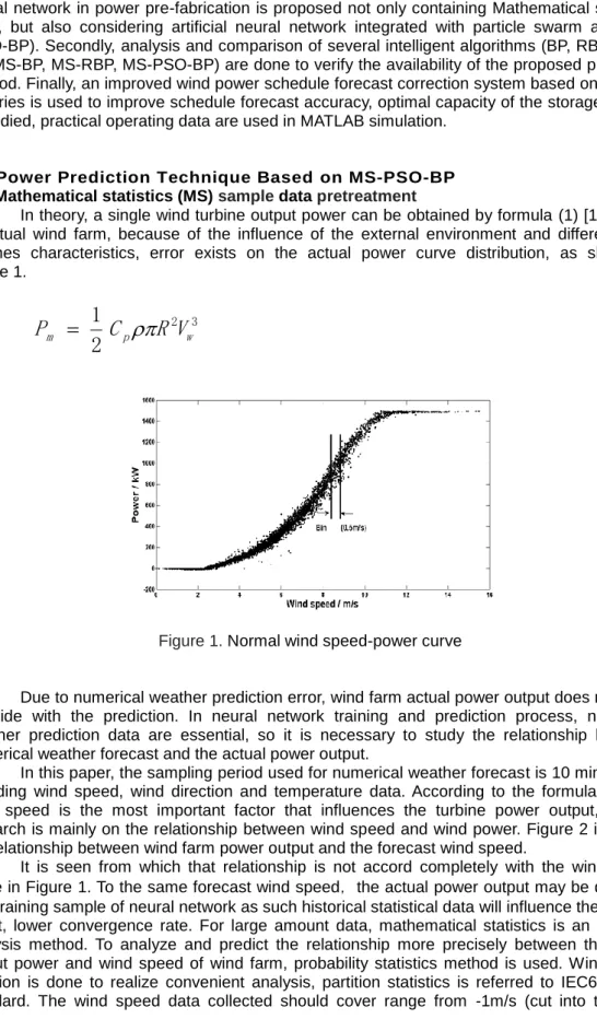
In theory, a single wind turbine output power can be obtained by formula (1) [19], while in actual wind farm, because of the influence of the external environment and different wind turbines characteristics, error exists on the actual power curve distribution, as shown in Figure 1. 3 2
2
1
w p mC
R
V
•P
(1)Figure 1. Normal wind speed-power curve
Due to numerical weather prediction error, wind farm actual power output does not quite coincide with the prediction. In neural network training and prediction process, numerical weather prediction data are essential, so it is necessary to study the relationship between numerical weather forecast and the actual power output.
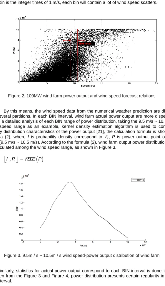
In this paper, the sampling period used for numerical weather forecast is 10 min, mainly including wind speed, wind direction and temperature data. According to the formula (1), the wind speed is the most important factor that influences the turbine power output, so the research is mainly on the relationship between wind speed and wind power. Figure 2 is shown the relationship between wind farm power output and the forecast wind speed.
It is seen from which that relationship is not accord completely with the wind power curve in Figure 1. To the same forecast wind speed,the actual power output may be different. The training sample of neural network as such historical statistical data will influence the training effect, lower convergence rate. For large amount data, mathematical statistics is an effective analysis method. To analyze and predict the relationship more precisely between the actual output power and wind speed of wind farm, probability statistics method is used. Wind speed partition is done to realize convenient analysis, partition statistics is referred to IEC61400-12 standard. The wind speed data collected should cover range from -1m/s (cut into the wind
speed) to 1.5 m/s multiplied by 85% of the rated wind speed. According to Bin methods [20], wind speed range collected is adopted 2 m/s to 20 m/s, divided by 1 m/s,the center value of each bin is the integer times of 1 m/s, each bin will contain a lot of wind speed scatters.
Figure 2. 100MW wind farm power output and wind speed forecast relations
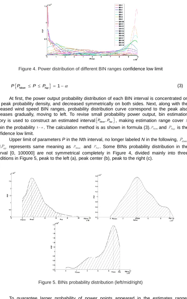
By this means, the wind speed data from the numerical weather prediction are divided into several partitions. In each BIN interval, wind farm actual power output are more dispersed. To get a detailed analysis of each BIN range of power distribution, taking the 9.5 m/s ~ 10.5 m/s wind speed range as an example, kernel density estimation algorithm is used to compute density distribution characteristics of the power output [21], the calculation formula is shown in formula (2), where f is probability density correspond to Pi, P is power output point of BIN
range(9.5 m/s ~ 10.5 m/s). According to the formula (2), wind farm output power distribution can be calculated among the wind speed range, as shown in Figure 3.
,
if P
KSDE P
(2)Figure 3. 9.5m / s ~ 10.5m / s wind speed-power output distribution of wind farm
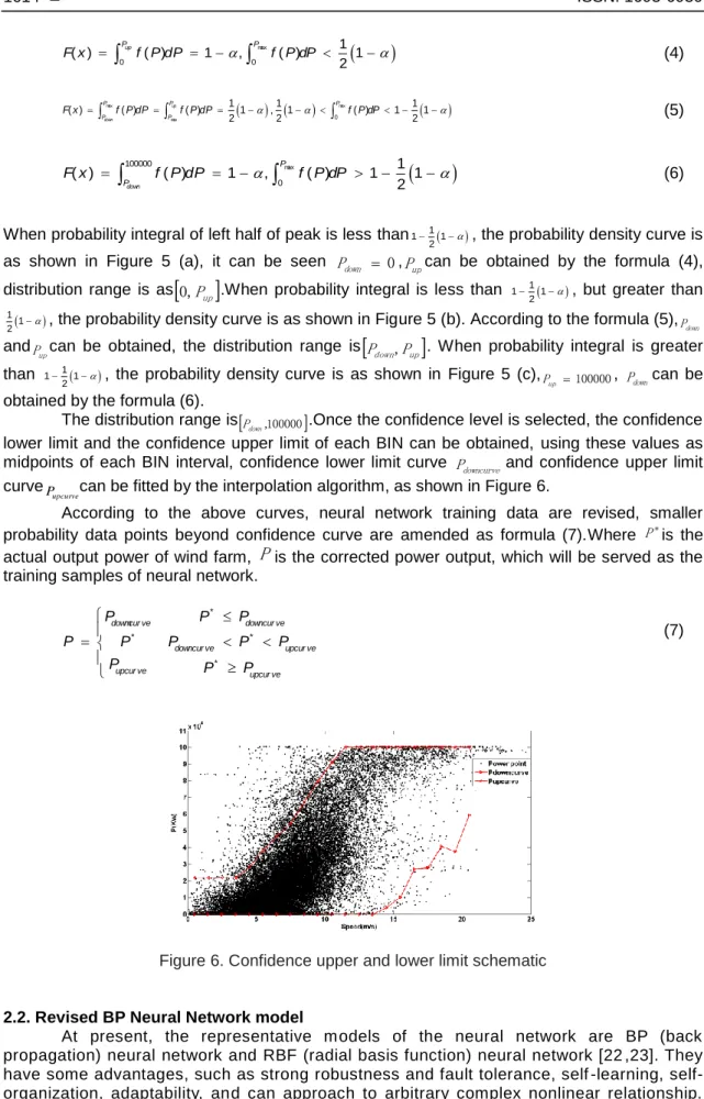
Similarly, statistics for actual power output correspond to each BIN interval is done, it can be seen from the Figure 3 and Figure 4, power distribution presents certain regularity in each BIN interval.
Figure 4. Power distribution of different BIN ranges confidence low limit
Ndown Nup
1P P P P (3) At first, the power output probability distribution of each BIN interval is concentrated on the peak probability density, and decreased symmetrically on both sides. Next, along with the increased wind speed BIN ranges, probability distribution curve correspond to the peak also increases gradually, moving to left. To revise small probability power output, bin estimation theory is used to construct an estimated intervalPNdown,PNup, making estimation range cover P
within the probability 1. The calculation method is as shown in formula (3).PNdownand PNup is the confidence low limit.
Upper limit of parameters P in the Nth interval, no longer labeled N in the following, Pdown
andPup represents same meaning as PNdown and PNup. Some BINs probability distribution in the
interval [0, 100000] are not symmetrical completely in Figure 4, divided mainly into three conditions in Figure 5, peak to the left (a), peak center (b), peak to the right (c).
Figure 5. BINs probability distribution (left/mid/right)
To guarantee larger probability of power points appeared in the estimates range, considering the probability symmetry distribution on both sides of the peak, the formula (4) (5) (6) are adopted to estimate intervals of above three conditions respectively.
max 0 0 1 ( ) ( ) 1 , ( ) 1 2 up P P F x
f P dP
f P dP (4) max max max 0 1 1 1 ( ) ( ) ( ) 1 , 1 ( ) 1 1 2 2 2 up down P P P P P F x f P dP f P dP f P dP (5)
max 100000 0 1 ( ) ( ) 1 , ( ) 1 1 2 down P P F x
f P dP
f P dP (6)When probability integral of left half of peak is less than 1
1 1
2
, the probability density curve is as shown in Figure 5 (a), it can be seen Pdown 0,Pupcan be obtained by the formula (4), distribution range is as
0,Pup
.When probability integral is less than 1 1 1
2
, but greater than
1 1
2 , the probability density curve is as shown in Figure 5 (b). According to the formula (5),Pdown
andPupcan be obtained, the distribution range is
Pdown,Pup
. When probability integral is greater than 1 1 1
2
, the probability density curve is as shown in Figure 5 (c),Pup 100000, Pdowncan be
obtained by the formula (6).
The distribution range is
Pdown,100000
.Once the confidence level is selected, the confidencelower limit and the confidence upper limit of each BIN can be obtained, using these values as midpoints of each BIN interval, confidence lower limit curve Pdowncurve and confidence upper limit curve
upcurve
P can be fitted by the interpolation algorithm, as shown in Figure 6.
According to the above curves, neural network training data are revised, smaller probability data points beyond confidence curve are amended as formula (7).Where P*is the actual output power of wind farm,
P
is the corrected power output, which will be served as the training samples of neural network.* * * * dowmcur ve downcur ve downcur ve upcur ve upcur ve upcur ve P P P P P P P P P P P (7)
Figure 6. Confidence upper and lower limit schematic
2.2. Revised BP Neural Network model
At present, the representative models of the neural network are BP (back propagation) neural network and RBF (radial basis function) neural network [22 ,23]. They have some advantages, such as strong robustness and fault tolerance, self -learning, self-organization, adaptability, and can approach to arbitrary complex nonlinear relationship.
The paper used them in wind power prediction, and prediction effects are compared and analyzed with each other.
2.2.1. BP neural network model
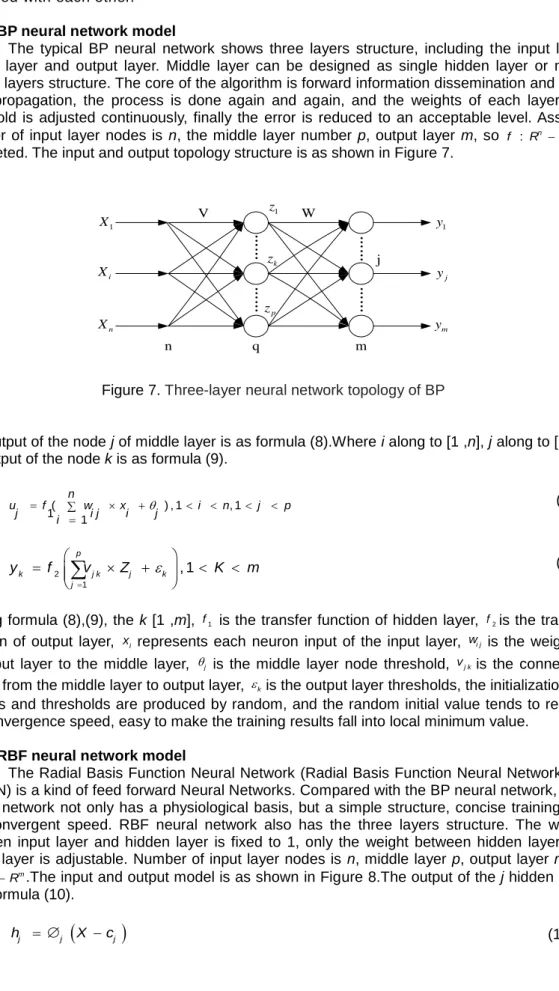
The typical BP neural network shows three layers structure, including the input layer, middle layer and output layer. Middle layer can be designed as single hidden layer or multi-hidden layers structure. The core of the algorithm is forward information dissemination and error back propagation, the process is done again and again, and the weights of each layer and threshold is adjusted continuously, finally the error is reduced to an acceptable level. Assume number of input layer nodes is n, the middle layer number p, output layer m, so f : Rn Rm is
completed. The input and output topology structure is as shown in Figure 7.
… … … … … … n q m … … W V j 1 X i X n X 1 z k z p z 1 y j y m y
Figure 7. Three-layer neural network topology of BP
The output of the node j of middle layer is as formula (8).Where i along to [1 ,n], j along to [1 ,p], the output of the node k is as formula (9).
n u f w x i n j p j i j i j i ) , ( 1 , 1 1 1 (8) 2 1 , 1 p k j k j k j y f v Z K m
(9)Among formula (8),(9), the k [1 ,m], f1 is the transfer function of hidden layer, f2is the transfer
function of output layer, xi represents each neuron input of the input layer, wi j is the weight of
the input layer to the middle layer, j is the middle layer node threshold, vj kis the connection
weight from the middle layer to output layer, kis the output layer thresholds, the initializations of
weights and thresholds are produced by random, and the random initial value tends to reduce the convergence speed, easy to make the training results fall into local minimum value.
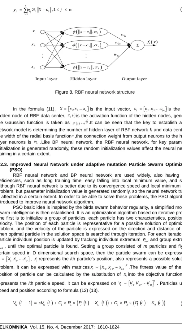
2.2.2. RBF neural network model
The Radial Basis Function Neural Network (Radial Basis Function Neural Network, the RBFNN) is a kind of feed forward Neural Networks. Compared with the BP neural network, RBF neural network not only has a physiological basis, but a simple structure, concise training and fast convergent speed. RBF neural network also has the three layers structure. The weight between input layer and hidden layer is fixed to 1, only the weight between hidden layer and output layer is adjustable. Number of input layer nodes is n, middle layer p, output layer m, so
: n m
f R R .The input and output model is as shown in Figure 8.The output of the j hidden node is as formula (10).
j j j
1 m , 1 h j i j i j i y w X c j
(11)…
Input layer Hidden layer Output layer
…
x c1 , 1
x c2 , 2
x ck , k
1 x 2 x p x 1i w 2i w ki w i f xFigure 8. RBF neural network structure
In the formula (11),X x x1, 2xnis the input vector, cj cj1,cj2cj nis the first j
hidden node of RBF data center. j is the activation function of the hidden nodes, generally,
the Gaussian function is taken as 22
u
u e
.It can be seen that the key to establish a RBF network model is determining the number of hidden layer of RBF network h and data center cj ,
the width of the radial basis functionσ,the connection weight from output neurons to the hidden
layer neurons is wi j .Like BP neural network, the RBF neural network, for key parameters,
initialization is generated randomly, these random initialization values affect the neural network training in a certain extent.
2.2.3. Improved Neural Network under adaptive mutation Particle Swarm Optimization (PSO)
RBF neural network and BP neural network are used widely, also having some deficiencies, such as long training time, easy falling into local minimum value, and so on. Although RBF neural network is better due to its convergence speed and local minimum value problem, but parameter initialization value is generated randomly, so the neural network training is affected in a certain extent. In order to be able to solve these problems, the PSO algorithm is introduced to improve neural network algorithm.
PSO basic idea is inspired by the birds swarm behavior regularity, a simplified model of swarm intelligence is then established. It is an optimization algorithm based on iterative process. The first is to initialize a group of particles, each particle has two characteristics, position and velocity. The position of each particle is representative for a possible solution of optimization problem, and the velocity of the particle is expressed on the direction and distance of flight. Then optimal particle in the solution space is searched through iteration. For each iteration, the particle individual position is updated by tracking individual extremum Pbest and group extremum
best
G , until the optimal particle is found. Setting a group consisted of m particles and fly at a certain speed in D dimensional search space, then the particle swarm can be expressed on
1, 2, D
X X X X , Xirepresents the ith particle's position, also represents a possible solution of problem, it can be expressed with matrices 1, 2,
T
i i i i D
X X X X .The fitness value of the each position of particle can be calculated by the substitution of Xiinto the objective function. Pbest represents the ith particle speed, it can be expressed on 1, 2,
T i i i i D
V V V V . Particles update speed and position according to formula (12) (13).
1
1 1
2 2
i j i j j i j j i j
1
1
i j i j i j
X t X t V t (13) Among formula (12) (13), j = 1, 2,..., d, represents particle dimension, t is the times of iteration, C1 and C2 are learning factors,R1andR2represent random number between 0~1, as inertia weight,Vi j
t represents the ith particle current speed in the tth generation, Xi j
trepresents the ith particle current location in the tth generation. In the general PSO algorithm, inertia weight represents the impact of the historical rate on the current speed. Where the larger is, the stronger global search ability particles have. While the lower is, the stronger portion search ability particles have. Once 0, it means that the particles lose ‘memory’. To give attention to both global and local search, take as linear gradient, in formula (14), i t er is current iteration number, i t ermaxis the maximum number of iterations, maxis inertia weight initial
value, mi nrepresents inertia weight ultimate value. To prevent particles from blind search, the particle's position and speed are limited respectively within a certain range[Xmax,Xmax] and
[Vmax,Vmax].
max max mi n max i t er i t er
(14)In order to avoid the ‘precocity’ and low iterative efficiency of PSO algorithm, the mutation is introduced to PSO algorithm, the principle is that the population is initialized at certain probability after each updating, so expanding search space of the dwindling population during the process of iteration, ensure the optimal location be searched before jumping out, thus improving the global convergence of the algorithm.
2.2.4. BP Neural Network combined with PSO on prediction model
The improved PSO algorithm is used to optimize parameters of neural network prediction model [24]. The steps are as following. Step 1 Building particle swarm, a neural network topology structure is established according to the input and output sample. The parameters be to optimize are coded to the individual particles of real vector population.
Step 2 The initialization of particle swarm parameters, mainly including the size of the population, learning factor, particle position and velocity interval, number of iterations, etc. Step 3 Calculating the particle fitness value, according to the input and output sample, the fitness function value of each particle is calculated, the current position is set to itself optimal location, the position of optimal particle in initialization population is set to the global optimal position. Step 4 Loop iteration, PSO algorithm formula (12) (13) are used to update particle velocity and position.
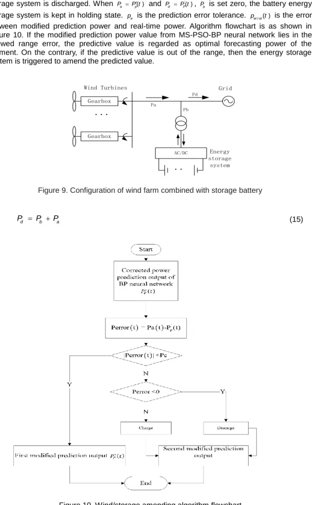
3. Wind/Storage Dynamic Correction of Schedule Forecast
It can be seen from literatures that prediction error exists inevitably in theoretical prediction algorithms due to various complex factors. The storage system can be used to absorb the redundant energy, correct unforeseen owed power supply, lower prediction errors and improve the accuracy of wind power forecast due to flexible charge-discharge characteristic. In Figure 9, the wind/storage system is mainly composed of wind turbines and vanadium battery package. The power relationship is as shown in formula (15). Where, Pais the actual power output of the wind farm, Pbis charging and discharging power of battery energy
storage system,Pd is the whole Wind/Storage system output.
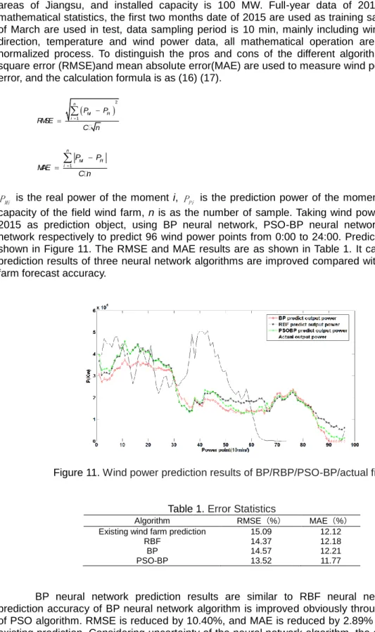
The key is how to determine Pb dynamically. From the foregoing description, MS-PSO-BP neural networks has been used to give modified predicted power '
) (
P
P t firstly, once the actual power output is greater than the predicted wind farm output (Pa P tp( )), then the energy storage system is charged to guarantee the accuracy of the forecast wind power (Pd P tp( )), andPbis set to a negative value. On the contrary, when Pa P tp( ), Pbis set to a positive value, the energy
storage system is discharged. When Pa P tp( ) and
'
( )
d P
P P t , Pb is set zero, the battery energy
storage system is kept in holding state. pe is the prediction error tolerance. per r or( )t is the error
between modified prediction power and real-time power. Algorithm flowchart is as shown in Figure 10. If the modified prediction power value from MS-PSO-BP neural network lies in the allowed range error, the predictive value is regarded as optimal forecasting power of the moment. On the contrary, if the predictive value is out of the range, then the energy storage system is triggered to amend the predicted value.
Gearbox Gearbox
...
AC/DC..
Pa Pb Pd Wind Turbines Energy storage system GridFigure 9.Configuration of wind farm combined with storage battery
d b a
P P P (15)
4. Simulation and Analysis
4.1. BP/RBP/PSO-BP prediction without training sample pretreatment
In order to verify the effectiveness of the proposed method, a real wind farm data samples are used to test the validity of the algorithm, the wind farm is located in the coastal areas of Jiangsu, and installed capacity is 100 MW. Full-year data of 2014 are used in mathematical statistics, the first two months date of 2015 are used as training sample, the data of March are used in test, data sampling period is 10 min, mainly including wind speed, wind direction, temperature and wind power data, all mathematical operation are performed by normalized process. To distinguish the pros and cons of the different algorithms, root mean square error (RMSE)and mean absolute error(MAE) are used to measure wind power prediction error, and the calculation formula is as (16) (17).
2 1 n Mi Pi i P P RMSE C n (16) 1 n Mi Pi i P P MAE C n
(17) MiP is the real power of the moment i, PPi is the prediction power of the moment i, C is power capacity of the field wind farm, n is as the number of sample. Taking wind power on March 1, 2015 as prediction object, using BP neural network, PSO-BP neural network, RBF neural network respectively to predict 96 wind power points from 0:00 to 24:00. Prediction results are shown in Figure 11. The RMSE and MAE results are as shown in Table 1. It can be seen that prediction results of three neural network algorithms are improved compared with existing wind farm forecast accuracy.
Figure 11.Wind power prediction results of BP/RBP/PSO-BP/actual field
Table 1.Error Statistics
Algorithm RMSE (%) MAE(%)
Existing wind farm prediction 15.09 12.12
RBF 14.37 12.18
BP 14.57 12.21
PSO-BP 13.52 11.77
BP neural network prediction results are similar to RBF neural network, but the prediction accuracy of BP neural network algorithm is improved obviously through amendment of PSO algorithm. RMSE is reduced by 10.40%, and MAE is reduced by 2.89% compared with existing prediction. Considering uncertainty of the neural network algorithm, the above methods are tested repeatedly, prediction results are analyzed. The wind farm power output are predicted
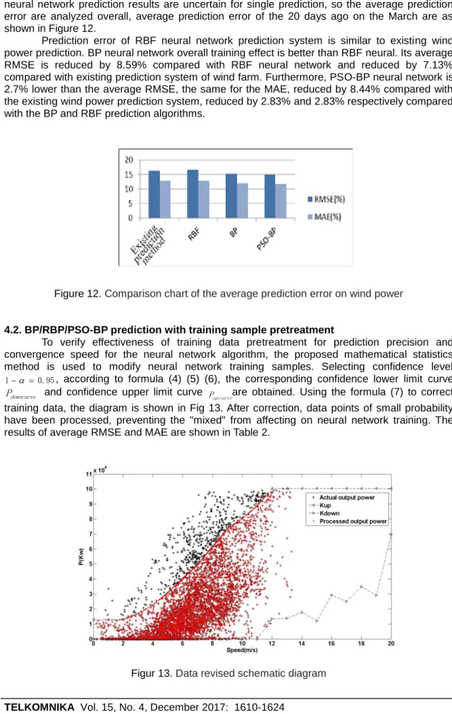
from March 1 to March 20, and the RMSE and MAE results are as shown in Appendix Table 1 and Appendix Table 2. It can be seen that RBF neural network, BP neural network and PSO-BP neural network prediction results are uncertain for single prediction, so the average prediction error are analyzed overall, average prediction error of the 20 days ago on the March are as shown in Figure 12.
Prediction error of RBF neural network prediction system is similar to existing wind power prediction. BP neural network overall training effect is better than RBF neural. Its average RMSE is reduced by 8.59% compared with RBF neural network and reduced by 7.13% compared with existing prediction system of wind farm. Furthermore, PSO-BP neural network is 2.7% lower than the average RMSE, the same for the MAE, reduced by 8.44% compared with the existing wind power prediction system, reduced by 2.83% and 2.83% respectively compared with the BP and RBF prediction algorithms.
Figure 12. Comparison chart of the average prediction error on wind power
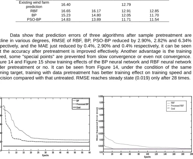
4.2. BP/RBP/PSO-BP prediction with training sample pretreatment
To verify effectiveness of training data pretreatment for prediction precision and convergence speed for the neural network algorithm, the proposed mathematical statistics method is used to modify neural network training samples. Selecting confidence level
95 . 0
1 , according to formula (4) (5) (6), the corresponding confidence lower limit curve downcurve
P and confidence upper limit curve Pupcurveare obtained. Using the formula (7) to correct training data, the diagram is shown in Fig 13. After correction, data points of small probability have been processed, preventing the "mixed" from affecting on neural network training. The results of average RMSE and MAE are shown in Table 2.
Table 2.Prediction Error Comparison Before and After the Training Data Pretreatment
Algorithm RMSE(%) RMSE(%)
Date revised MAE(%)
MAE(%)
Date revised Existing wind farm
prediction 16.40 12.79
RBF 16.65 16.17 12.91 12.85
BP 15.23 14.80 12.05 11.70
PSO-BP 14.83 13.89 11.71 11.54
Data show that prediction errors of three algorithms after sample pretreatment are decline in various degrees, RMSE of RBF, BP, PSO-BP reduced by 2.90%, 2.82% and 6.34% respectively, and the MAE just reduced by 0.4%, 2.90% and 0.4% respectively, it can be seen that the accuracy after pretreatment is improved effectively. Another advantage is the training speed, some "special points" are prevented from slow convergence or even not convergence. Figure 14 and Figure 15 show training effects of the BP neural network and RBF neural network under pretreatment or no. It can be seen from Figure 14, under the condition of the same training target, training with data pretreatment has better training effect on training speed and precision compared with that untreated. RMSE reaches steady state (0.019) only after 28 times.
Figure 14. BP neural network training with and
without data pretreatment Figure 15.and without RBF neural network training with data pretreatment
While without data pretreatment, it needs 46 times training and RMSE reaches the steady state (0.024). It can also be seen from the Figure 15, under the condition of the same training target, RBF neural network training after data pretreatment need only 23 times to reach the target value of 0.01. Without pretreatment, no training goals can be arrived even after a maximum of 200 times. Comparing Figure 14 with Figure 15, it can also be seen that algorithms convergence speed and convergence results of BP are all inferior to that of RBF, showing feasibility and effectiveness of the experimental results.
4.3. Wind/storage system physical amending for schedule forecast
The simulation experiment is done in a wind farm of 100000 kilowatts in eastern coastal of China. The historical statistical data are concluded within 4 consecutive days in June, such as wind speed, the wind field actual output power. The data during previous two days are adopted as training samples for prediction model. The measured data in the next two days are regarded as the calibration data, which are used to verify the accuracy and yet the validity of the algorithm.
The results of simulation are shown in Figure 16. Prediction errors simulation are as the basis to determine the battery capacity needed. In order to prevent the prediction process from the occasional error, experiments are conducted 1000 times, each maximum capacityCmaxof
battery charge or discharge is stated, and a high level of confidence Cmax is selected for
referenced battery capacity. When certain capacity is supplied in the wind power system, the
5 10 15 20 25 30 35 40 45 50 55 60 0 0.02 0.04 0.06 0.08 0.1 0.12 Epochs M e a n S q u a r e d E r r o r ( m s e ) BP Processed BP Goal 0 20 40 60 80 100 120 140 160 180 200 0.01 0.015 0.02 0.025 0.03 0.035 0.04 0.045 0.05 0.055 Epochs M e a n S q u a a r e d E r r o r ( m s e ) RBF Processed RBF Goal
results of reducing the prediction errors are as shown in Figure 17 and Figure 18. As can be seen from Figure 17, the power output Pd of the wind farm is smooth more with battery energy storage system, and is close to the prediction curve of wind power. Figure 18 shows that the battery capacity can also meet the needs of short-term wind power correction. Meanwhile, it is concluded from the experiments that RMSE of wind power forecast has been reduced to 9.3535e+003W, 10 minutes predictive error integration is reduced to 2.1941e+004Ah, the battery energy storage system can minify wind power prediction error effectively.
Figure 16. Modified Power prediction error integration
Figure 17. Power output forecast correction with battery energy storage
Figure 18. Storage battery SOC change during correction
5. Conclusion
This paper combines the mathematical statistics and BP neural network on wind power prediction, PSO algorithm is used to improve prediction precision. Based on which, Wind/Storage system is used to amend wind farm power forecast. Simulation results show that the proposed pretreatment (mathematical statistics method) can improve the neural network training speed and precision. In addition, the PSO algorithm can also improve the prediction precision of the BP neural network effectively. Compared with the current wind farm forecasting strategy, RMSE of PSO-BP can be reduced by 6.34%, and the MAE reduced by 0.4%. Moreover, the schedule forecast accuracy can be improved effectively by physical Wind/Storage dynamical correction, and experiments show that RMSE of wind power forecast has been reduced to 9.3535e+003W, the energy storage system can minify wind power prediction error effectively. However, limited by the technical conditions, the battery capacity is still an important bottleneck in application all along. The battery capacity can be insufficient for big share on the access of large wind farms, but it can be used as a power fine-tuning in large wind power.
0 20 40 60 80 100 120 140 160 180 200 -150 -100 -50 0 50 100 150 200 Time(T=15min) C apa c it y (M Ah) 0 50 100 150 0 20 40 60 80 100 Time(T=15min) P(M W )
Forecast corrected with battery Forecast corrected without battery
0 50 100 150 200 0 0.2 0.4 0.6 0.8 1 Time(T=15min) SOC
Acknowledgements
This work is a part of the Natural Science Foundation of China (No. 51377047,No.51407097). Experimental data are taken from Jiangsu Longyuan Wind Power Co., Ltd..The authors would like to thank for the supports from both the Ministry of Science and Technology of China and National Natural Science Foundation of China and Jiangsu Longyuan Wind Power Co., Ltd. of China.
References
[1] KM Nor. Renewable Distributed Generation Models in Three-Phase Load Flow Analysis for Smart Grid. Telkomnika. 2013; 11(4): 661-668.
[2] Tastu J, Pinson P, Trombe PJ, Madsen H. Probabilistic forecasts of wind power generation accounting for geographically dispersed information. IEEE Transactions on Smart Grid. 2014; 1: 480-489.
[3] Quan H, Srinivasan D, Khosravi A. Short-term load and wind power forecasting using Neural Network-based prediction intervals. IEEE Transactions on Neural Networks and Learning Systems.
2014; 2: 303-315.
[4] Venayagamoorthy GK, Rohrig K, Erlich I. One step ahead: short-term wind power forecasting and intelligent predicti-ve control based on data analytics. IEEE Power and Energy Magazine. 2012; 5: 70-78.
[5] Can W, Zhao X, Pinson P. Direct interval forecasting of wind power. IEEE Transactions on Power Systems. 2013; 4: 4877-4878.
[6] Ming Y, Shu F, Wei JL. Probabilistic short ter-m wind power forecast using componential sparse bayesian learning. IEEE Transactions on Industry Applications. 2013; 6: 2783-2792.
[7] Potter CW, Negnevitsky M. Very short-term wind forecasting for Tasmanian power generation. IEEE Transactions on Power Systems. 2006; 2: 965-972.
[8] Yongqian L, Jie S, Yongping Y, Wei JL. Short-term wind power prediction based on wavelet transform Support Vector Machine and Statistic-characteristics analysis. IEEE Transactions on Industry Applications. 2012, 4: 1136-1141.
[9] Abdollah KF, Abbas K, Saeid N. A New Fuzzy-Based Combined Prediction Interval for Wind Power Forecasting. IEEE Transactions on Power Systems. 2016; 1: 18-26.
[10] Rasit A. Artificial neural networks applications in wind energy systems: a review. Renewable and Sustainable Energy Reviews. 2015; 49: 534–562.
[11] Tewari S, Geyer CJ, Mohan N. A Statistical model for wind power forecast error and its application to the estimation of penalties in liberalized markets. IEEE Transactions on Power Systems. 2011; 4: 2031-2039.
[12] Hamideh B, Saifur R, Manisa P. Sizing Energy Storage to Mitigate Wind Power Forecast Error Impacts by Signal Processing Techniques. IEEE Transactions on Sustainable Energy. 2015; 6(4):1457-1465.
[13] Li Q, Choi SS, Yuan Y, Yao DL. On the determination of battery energy storage capacity and short-term power Dispatch of a wind farm. IEEE Transactions on Sustainable Energy. 2011; 2: 148 -158. [14] Zheng X, Ding J, Li M, et al. Using STATCOM with Energy Storage to Enhance ACDC System
Stability. Telkomnika. 2016; 14(2): 423-430.
[15] Ogimi K, Yoza A, Yona A, et al. A study on optimum capacity of battery energy storage system for wind farm operation with wind power forecast data. Harmonics and Quality of Power (ICHQP), 2012 IEEE 15th International Conference on. IEEE.2012: 118-123.
[16] Mohod SW, Aware MV. Micro wind power generator with battery energy storage for critical load. IEEE Systems Journal. 2012; 1: 118-125.
[17] Teleke S, Baran M E, Bhattacharya S, et al. Optimal control of battery energy storage for wind farm dispatching. IEEE Transactions on Energy Conversion. 2010; 25(3): 787-794.
[18] D Kottick, Blau M, Edelstein D. Battery energy storage for frequency regulation in an island power system. IEEE Transactions on Energy Conversion. 1993; 3: 455-459.
[19] Zhou S, Lu ZX. Wind power and electric power system. BeiJing: Chinese Electric Power Publishing house. 2011: 228.
[20] Kalavade A, Lee EA. The extended partitioning problem: hardware/software mapping and implementation-bin selection. IEEE Sixth International Workshop on Rapid System Prototyping. 1995: 12-18.
[21] Li CH, Sun ZH, et al. Kernel Density Estimation and its application to clustering algorithm construction. Journal of Computer Research and Development. 2004; 10.
[22] Cong S. Toolbox for MATLAB neural network theory and application. BeiJing: China Science and Technology University Press. 1998.
[23] P Campolucci, A Uncini, Piazza F, Rao BD. On-line learning algorithms for locally recurrent neural networks. IEEE Transactions on Neural Networks. 1999;10(2): 253-271.
[24] Pingzhou T, Zhaocai X. The research on BP Neural Network model based on guaranteed convergence Particle Swarm Optimization. Second International Symposium on Intelligent Information Technology Application. 2008; 2: 13-16.
Appendix
Appendix Table 1 . RMSE Contrast of Algorithm Proposed on Paper with on-Site Original Forecast
Date Wind Forecasting System
Training data uncorrected Training data corrected
RBF BP PSO-BP RBF BP PSO-BP 3.1 15.09 14.37 14.56 13.51 15.46 14.41 14.31 3.2 11.54 11.73 12.37 9.99 12.44 12.65 9.95 3.3 24.69 25.32 21.63 20.14 23.18 20.27 20.96 3.4 24.15 20.36 24.39 23.25 21.60 23.71 21.18 3.5 10.51 15.30 13.26 18.82 12.36 12.30 12.37 3.6 8.21 12.44 10.00 11.32 6.22 11.61 9.69 3.7 7.74 10.88 8.74 10.76 6.96 8.11 9.03 3.8 33.46 33.20 33.24 32.77 33.73 33.76 30.99 3.9 21.99 27.73 14.90 12.82 21.86 13.38 13.72 3.1 36.35 28.47 22.44 19.33 24.02 20.04 22.01 3.11 4.63 6.93 5.20 3.74 5.79 6.48 5.12 3.12 14.5 14.44 12.14 12.56 11.70 1045 10.05 3.13 12.17 12.06 13.27 12.88 25.63 13.44 10.54 3.14 12.16 12.03 14.35 9.39 12.24 13.11 11.20 3.15 11.7 14.89 12.67 13.40 13.35 11.51 12.63 3.16 10.22 10.30 10.31 9.03 10.04 9.04 9.02 3.17 13.72 14.72 12.60 15.73 11.44 13.33 12.42 3.18 33.56 28.01 25.24 28.21 29.42 27.59 21.87 3.19 13.3 12.23 12.91 10.74 11.93 11.70 12.60 3.20 8.21 7.64 10.25 8.13 13.94 9.08 8.13 Mean 16.395 16.65 15.23 14.83 16.17 14.80 13.89
Appendix Table 2. MAE Contrast of Algorithm Proposed on Paper with on-Site Original Forecast
Date Wind Forecasting System
Training data uncorrected Training data corrected
RBF BP PSO-BP RBF BP PSO-BP 3.1 12.12 12.18 11.59 11.46 12.18 12.14 12.42 3.2 8.94 9.24 9.37 10.05 9.06 8.67 10.25 3.3 18.56 22.61 16.39 16.67 22.72 15.83 17.47 3.4 16.81 16.28 22.35 20.71 16.19 18.75 19.47 3.5 8.22 12.74 10.84 11.22 12.24 11.20 8.52 3.6 7.07 9.98 7.94 8.81 9.49 8.79 8.98 3.7 5.41 6.11 7.59 6.06 5.89 6.12 2.35 3.8 26.20 26.68 26.53 27.36 26.88 24.81 26.78 3.9 18.80 17.93 11.22 9.82 18.53 11.11 10.55 3.1 25.01 19.92 9.85 14.44 20.07 15.73 15.47 3.11 3.37 5.71 5.20 3.71 4.66 3.96 4.84 3.12 11.44 13.04 9.01 10.74 12.85 7.63 8.35 3.13 9.91 8.15 14.25 9.12 9.00 10.06 9.92 3.14 9.71 8.35 9.95 9.37 8.32 11.09 11.16 3.15 10.05 12.16 12.84 9.95 12.00 11.36 9.54 3.16 8.23 7.83 7.32 6.85 7.76 6.62 7.17 3.17 11.67 12.45 9.80 9.44 12.41 9.69 10.83 3.18 27.87 23.01 23.18 21.52 22.99 23.79 19.09 3.19 10.66 8.80 9.30 10.45 8.77 10.05 8.90 3.2 5.68 5.04 6.51 6.47 5.08 6.66 8.82 Mean 12.79 12.91 12.05 11.71 12.85 11.70 11.54