Simulation Sampling with Live-points
Thomas F. Wenisch
Roland E. Wunderlich
Babak Falsafi
James C. Hoe
Computer Architecture Laboratory (CALCM) Carnegie Mellon University, Pittsburgh, PA 15213-3890
{rolandw, twenisch, babak, jhoe}@ece.cmu.edu
http://www.ece.cmu.edu/~simflex
ABSTRACT
Current simulation-sampling techniques construct accurate model state for each measurement by continuously warming large microar-chitectural structures (e.g., caches and the branch predictor) while functionally simulating the billions of instructions between measure-ments. This approach, called functional warming, is the main perfor-mance bottleneck of simulation sampling and requires hours of runtime while the detailed simulation of the sample requires only minutes. Existing simulators can avoid functional simulation by jumping directly to particular instruction stream locations with architectural state checkpoints. To replace functional warming, these checkpoints must additionally provide microarchitectural model state that is accurate and reusable across experiments while meeting tight storage constraints.
In this paper, we present a simulation-sampling framework that replaces functional warming with live-points without sacrificing accuracy. A live-point stores the bare minimum of functionally-warmed state for accurate simulation of a limited execution window while placing minimal restrictions on microarchitectural configura-tion. Live-points can be processed in random rather than program order, allowing simulation results and their statistical confidence to be reported while simulations are in progress. Our framework matches the accuracy of prior simulation-sampling techniques (i.e., ±3% error with 99.7% confidence), while estimating the performance of an 8-way out-of-order superscalar processor running SPEC CPU2000 in 91 seconds per benchmark, on average, using a 12 GB live-point library.
1. INTRODUCTION
Computer architecture research routinely employs detailed cycle-accurate simulation to explore and validate microarchitectural inno-vations. Ideally, simulation studies should use the same benchmarks used to assess real hardware. Unfortunately, benchmark applications that are tuned to run for minutes on real hardware can require over a month to execute on today’s high performance microarchitecture simulators [2,11,26,30].
Past research advocates sampling [5,9,19,20,32,37,38]—that is, measuring only a subset of benchmark execution—as a technique to accelerate microarchitecture simulation. Many such studies advocate uniform sampling using rigorous statistical theory [5,9,20,37] to provide explicit validation that the measured portions accurately represent the behavior of a benchmark.
A recent study of prevailing simulation-sampling approaches by Yi et al. [38] concluded that the SMARTS simulation-sampling approach [37] provides the highest estimation accuracy. The SMARTS design minimizes instructions simulated by measuring a large number (e.g., 10,000) of brief (e.g., 1000-instruction) simulation windows.
SMARTS avoids measurement error from cold state by continuously warming large microarchitectural structures (e.g., caches and the branch predictor) while functionally simulating the billions of instructions between measurements, a warming strategy referred to as functional warming.
Although functional warming enables accurate performance estima-tion, it limits SMARTS’s speed, occupying more than 99% of simula-tion runtime. Funcsimula-tional warming dominates simulasimula-tion time because the entire benchmark’s execution must be functionally simulated, even though only a tiny fraction of the execution is simulated using detailed microarchitecture timing models.
The second shortcoming of SMARTS is that functional warming requires simulation time proportional to benchmark length rather than sample size. As a result, the overall runtime of a SMARTS exper-iment remains constant even when the measured sample size is reduced by relaxing an experiment’s statistical confidence require-ments or through recently-proposed sampling optimizations such as matched-pair comparison [9] and stratified sampling [36]. Moreover, functional warming time will increase with the advent new bench-mark suites, such as SPEC CPU2006, that lengthen benchbench-marks to scale with hardware performance improvement [33]. Optimizations that accelerate functional warming, such as direct execution [4], do not improve SMARTS’s scaling behavior.
In this paper, we propose live-points as a replacement for functional warming to provide reduced simulation turnaround time, propor-tional to sample size, without sacrificing accuracy. A live-point stores the necessary data to reconstruct warm state for a simulation sampling execution window. Although modern computer architecture simulators frequently provide checkpoint creation and loading capa-bilities [2,23], current checkpoint implementations: (1) do not provide complete microarchitectural model state, and (2) cannot scale to the required checkpoint library size (~10,000 checkpoints per benchmark) because of multi-terabyte storage requirements. We address the first limitation of conventional checkpoints by storing selected microarchitectural state in live-points, an approach we call checkpointed warming.The key challenge of checkpointed warming lies in storing microarchitectural state such that live-points can still simulate the range of microarchitectural configurations of interest. Fortunately, previous studies have shown that, with the exception of the branch predictor and memory hierarchy, the vast majority of microarchitectural state can be reconstructed dynamically with minimal simulation (a few thousand instructions), and thus need not be stored [37]. For the exceptional structures, researchers can often place limits on the configurations of interest (e.g., through trace-based studies). We design checkpointed warming to reproduce these structures under user-specified limits.
We reduce the size of conventional checkpoints by three orders of magnitude through storing in live-points only the subset of state
necessary for limited execution windows, an approach we call live-state. Live-state exploits the brevity of simulation sampling execu-tion windows (thousands of instrucexecu-tions) to omit the vast majority of state. The minimal state subset can be known a priori only for the commit instruction stream, and is not known for wrong-path (specu-lative) instructions. However, whereas wrong-path instruction latency affects scheduling through pipeline resource contention, wrong-path operand values rarely affect instruction throughput. We exploit this observation by storing only the state required for correct path execution and approximate wrong-path scheduling.
We present results from a live-point-enabled simulator derived from SimpleScalar 3.0 sim-outorder [2] simulating the execution of the SPEC CPU2000 (SPEC2K) benchmarks on two microarchitec-tural configurations to show:
•Accelerated simulation with practical storage. Live-point simulation sampling is over 250times faster than existing simu-lation sampling approaches (on average 91 seconds per bench-mark) for an 8-way out-of-order superscalar while maintaining the estimated CPI error at ±3% with 99.7% confidence. Although functional warming produces an aggregate of 36 TB of state while sampling SPEC2K, a gzip-compressed SPEC2K live-point library supporting 1 MB caches requires just 12 GB of storage. •Parallel simulation and online results. We construct
indepen-dent live-points that can be processed in parallel and in an arbi-trary order. By randomizing the processing order, we can report unbiased results and their statistical confidence continuously during simulation. As more live-points are processed, results converge toward their final values and confidence improves. In contrast, simulators that use functional warming cannot report results until simulation is complete and require strict program-order simulation to allow for unbiased sampling, preventing parallel simulation.
• Reusable live-point libraries. We ensure reusability of a fixed-size live-point library across comparative performance studies that have unpredictable sample size requirements using matched-pair sample comparison. Individual live-points can simulate a wide range of microarchitectural configurations using our check-pointed warming approach. Our live-points constrain only the configuration of the branch predictor (to a user-selected set of alternatives) and the cache/TLB hierarchy (through user-selected upper bounds on size and associativity). Our results demonstrate that checkpointed warming is more accurate (1.6% worst-case CPI bias) than currently-known checkpoint-based alternatives that do not constrain microarchitectural configuration (5.4% worst-case CPI bias).
This paper is organized as follows. Section 2 presents background on functional warming. We present our methodology in Section 3. In Section 4, we compare checkpointed warming to alternative warming methods in terms of accuracy, flexibility, and speed. We describe live-state, our storage approach for live-points, in Section 5, and present the live-point experiment framework in Section 6. Section 7
presents performance results and analysis. Related work is described in Section 8. We conclude in Section 9.
2. BACKGROUND
Simulation sampling derives estimates of performance (CPI, power, etc.) of benchmark applications on a simulated microarchitecture from measurements of a sample of the benchmark’s dynamic instruc-tion stream. By choosing the measured sample according to estab-lished statistical sampling methods [16], simulation sampling can rely on statistical measures of confidence to validate that estimated results represent the behavior of the full benchmark.
Although statistics provides us with probabilistic guarantees that esti-mated results are representative, these guarantees do not assure us that estimated results are error-free. Errors introduced into the indi-vidual measurements that make up a sample (e.g., by the measure-ment methodology) are referred to as bias, and are not accounted for by statistical confidence calculations. In simulation sampling, the most common cause of bias is the cold-start effect of unwarmed microarchitectural structures. For example, assuming empty caches may result in incorrectly low performance estimates.
The primary challenge in simulation sampling is to devise a strategy to construct accurate initial state rapidly. For each measurement, the simulator must construct both architectural state (e.g., register and memory values) and microarchitectural state (e.g., pipeline compo-nents and the cache hierarchy) to avoid cold-start bias. A recent survey of simulation sampling approaches [38] concluded that the SMARTS simulation sampling approach [37] provides the highest esti-mation accuracy.
SMARTS uses a two-tiered strategy to construct every measurement’s initial state as depicted in Figure 1. Prior to each measurement, microarchitectural structures for which current state reflects the history of a small, bounded set of recent instructions—such as the reorder buffer or issue queue—are warmed through detailed warm-ing: brief simulation (e.g., a few thousand instructions) of the complete detailed performance model sufficient to warm such small structures. We refer to adjacent detailed warming and measurement intervals as a detailed window.
The second component of the SMARTS warming strategy, functional warming, addresses state updates between two detailed windows. Like other simulation sampling frameworks [19,22,32,35], SMARTS functionally simulates each instruction to update architectural state. To minimize and bound detailed warming requirements, SMARTS continuously updates structures with microarchitectural state that persists across detailed windows—caches, TLBs, and branch predic-tors. These structures cannot be warmed sufficiently by a brief detailed warming period.
Unfortunately, as proposed, functional warming is a performance bottleneck in simulation sampling [12,37]. Given typical cycle-accu-rate simulation models (e.g., SimpleScalar sim-outorder [2]), the performance measurement of a wide-issue out-of-order
supersca-S
MARTSwarming strategy
…Functional warming
(~50x faster than detailed sim.)
Measurement
(~1000 instructions of detailed simulation)
Detailed warming (~2000 instructions of detailed simulation) Detailedwindow
lar processor using the SMARTS strategy requires little detailed simu-lation: typically about a minute on a modern host machine. A SMARTS-based simulator’s total runtime, however, is orders of magnitude longer because the functional warming between detailed windows dominates runtime.
Unlike functional warming, live-point simulation time is directly proportional to sample size. Sample size depends only on a proces-sor’s performance variability across a benchmark’s execution, and the desired statistical confidence [22,37].
3. METHODOLOGY
We evaluate live-points in a sampling simulator based on the SimpleScalar 3.0 sim-outorder simulator [2] for the Alpha ISA. We modify sim-outorder’s memory subsystem to include a store buffer and miss status holding registers (MSHRs), and model inter-connect bottlenecks in the memory hierarchy. We encode live-points using ASN.1 DER format [15] and gzip compression, which incur minimal storage and processing time overhead. We use all 26 SPEC2K benchmarks [13] and evaluate all reference inputs except vpr-place and three perlbmk inputs, as these inputs fail to simulate correctly in sim-outorder. Overall, we include 41 benchmark/ input set combinations in this study.
Without loss of generality, we use CPI (cycles-per-instruction) as our target metric for estimation. Simulation sampling, however, has been shown to be applicable to other performance metrics of choice [37, 38]. We measure CPI bias by averaging actual error (relative to full
sim-outorder simulations) over five different samples, according to the methodology described in [37].
We evaluate live-points with two microarchitectural configurations. Our baseline 8-way out-of-order superscalar model represents a processor in the current technology generation. The 16-way out-of-order superscalar configuration is included to reflect an aggressive future design point. This configuration has a wider datapath, larger out-of-order window, and larger caches, to exercise the effects of enlarged microarchitectural state. The details of the 8-way and 16-way configurations are summarized in Table 1.
We use the sampling approach from [37], periodic 1000-instruction measurement intervals, to identify measurement locations for all experiments. This sample design has been demonstrated to minimize the total number of instructions in detailed windows, and thus, detailed simulation time. However, live-points can also be applied to other sample designs (e.g., random sampling). We choose sample size to achieve precisely 99.7% confidence of ±3% error for each result.
We report simulation runtimes for systems with 2.80 GHz Intel Xeon (512 KB L2) processors.
4. WHY CHECKPOINTED WARMING?
Functional warming repeats architectural state updates across differ-ent simulations of the same benchmark. (Simulating workloads for which architectural state varies across repeated runs—i.e., because of interrupt timing or different interleaving of multiprocessor instruc-tion streams—is beyond the scope of this work.) Frequently, microar-chitectural state updates are also identical across runs. Checkpoints can memoize the redundant calculation across runs, amortizing the one-time cost of computing warmed state. We are interested in
finding the best way to take advantage of checkpoints to accelerate warming.
Although some microarchitecture studies have suggested or used checkpoints to accelerate simulation [1,9,10,28], none have explored the space of microarchitecture warming solutions in the context of checkpointing. For each portion of model state generated by func-tional warming, we may choose either to construct the state dynami-cally, or store it in checkpoints. This choice impacts simulation sampling along three dimensions: the accuracy of the warmed state, the reusability of checkpoints across microarchitectural configura-tions, and the speed of simulation. In this section, we explore the warming method design space with respect to these three dimensions and justify our choice of checkpointed warming to implement live-points.
4.1 Simulation sampling warming methods
There is a rich design space of possible warming strategies that combine checkpoints and dynamic warming for various portions of architectural and microarchitectural model state. We restrict our exploration to strategies that use detailed warming to initialize queue and pipeline state. Detailed warming can reconstruct state for the vast majority of microarchitectural structures rapidly, and the amount of required warming can be determined via worst-case analysis [37]. By warming most structures dynamically, we avoid storing any state for these structures, and do not constrain model parameters that affect this state.
Evaluation criteria. We focus our design exploration on warming alternatives for long-history structures, such as caches and branch predictors, for which detailed warming is prohibitively slow. We evaluate alternatives based on their accuracy, checkpoint reusability, and speed.
With respect to accuracy, we consider only the bias introduced by the warming strategy. SMARTS demonstrated low bias—0.6% on aver-age, 1.6% worst case [37]—using functional warming. It is essential
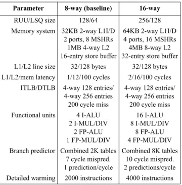
Table 1. Microarchitectural configurations.
Parameter 8-way (baseline) 16-way
RUU/LSQ size 128/64 256/128
Memory system 32KB 2-way L1I/D 2 ports, 8 MSHRs
1MB 4-way L2 16-entry store buffer
64KB 2-way L1I/D 4 ports, 16 MSHRs 4MB 8-way L2 32-entry store buffer L1/L2 line size 32/128 bytes 32/128 bytes L1/L2/mem latency 1/12/100 cycles 2/16/100 cycles
ITLB/DTLB 4-way 128 entries/ 4-way 256 entries 200 cycle miss
4-way 128 entries/ 4-way 256 entries 200 cycle miss Functional units 4 I-ALU
2 I-MUL/DIV 2 FP-ALU 1 FP-MUL/DIV 16 I-ALU 8 I-MUL/DIV 8 FP-ALU 4 FP-MUL/DIV Branch predictor Combined 2K tables
7 cycle mispred. 1 prediction/cycle
Combined 8K tables 10 cycle mispred. 2 predictions/cycle Detailed warming 2000 instructions 4000 instructions
to maintain this high accuracy when accelerating warming because we cannot detect bias through statistical confidence calculations. We evaluate the reusability of a warming methodology in terms of the restrictions it places on simulator configuration. When we store the warmed state of microarchitectural structures in a checkpoint, we may be forced to limit some of the configuration parameters for that structure.
Finally, we evaluate the speed of warming alternatives in two ways. First, we consider how fast measurements can be processed. For all alternatives, time to simulate the detailed window is the same, while functional warming and checkpoint decompression/loading time varies. Second, we consider whether detailed windows are indepen-dent, or must be simulated in program order. Independent windows can be simulated in parallel, and enable online reporting of measure-ment results.
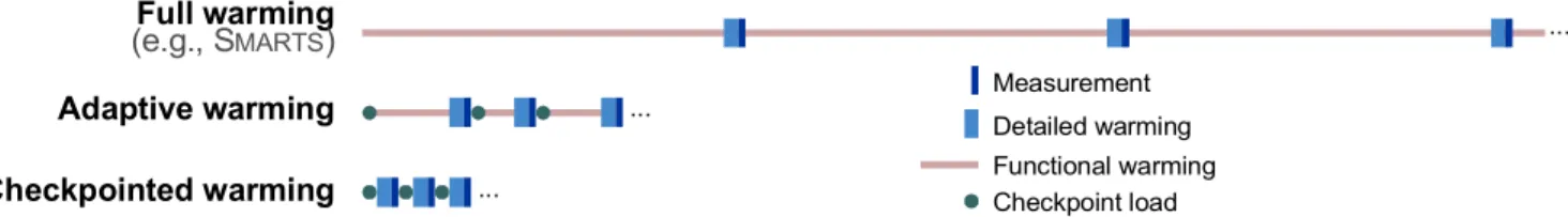
Warming methods. Figure 2 depicts alternatives in the warming strategy design space. At one extreme, functional warming is used for the entire duration between measurements, without checkpoints (as in SMARTS). We refer to this method as full warming. The opposite extreme, checkpointed warming,eliminates all functional warming and stores long-history state in checkpoints. This approach requires limiting some design parameters of the checkpointed structures. Functionally-warming microarchitectural state for the entire duration between measurements is usually not necessary. In adaptive warm-ing, we store architectural state in checkpoints, and reconstruct long-history state with a reduced functional warming period. Adaptive warming requires a mechanism to determine precisely how little functional warming each detailed window requires.
Trade-offs. Figure 3 illustrates the relationship between each warming alternative and our three evaluation criteria. Each alterna-tive optimizes for two of the design criteria (the two depicted nearest it), at the expense of the third.
Full warming maximizes accuracy and flexibility, but its need for long periods of functional warming makes it slow, and its turnaround time scales with benchmark length. As full warming requires no checkpoints, no configuration parameters are fixed.
Adaptive warming maintains the reusability of full warming and improves speed, but we show that it sacrifices accuracy. The accu-racy and speed of adaptive warming depend on a rigorous determina-tion of the minimal funcdetermina-tional warming period for each detailed window. Unfortunately, determining the correct amount of warming remains a difficult and unsolved problem [18].
Checkpointed warming matches the accuracy of full warming and maximizes speed, at the expense of checkpoint reusability. Check-pointed warming achieves this accuracy because it uses full warming simulation to generate the checkpointed state.
Because checkpointed warming spends no time performing func-tional warming, it is the fastest alternative. The drawback of check-pointed warming is that it imposes limits on some aspects of the simulated microarchitectural parameters (e.g., the maximum size or associativity of a cache), which constrains checkpoint reusability. Reusability is important because we must amortize the one-time cost of checkpoint creation (roughly the cost of a full-warming simula-tion) over a series of experiments.
Each of the three warming approaches suffers from a different key weakness. The speed of full warming has been quantified in [37]. We evaluate the accuracy of adaptive warming in Section 4.2. We then explore the reusability of checkpointed warming in Section 4.3.
4.2 Adaptive warming
The key challenge of achieving accuracy with adaptive warming lies in determining the functional warming period length. If the warming period is underestimated, simulation results will be biased. If the warming period is overestimated, we sacrifice simulation speed. A recently-proposed technique for determining cache warming requirements is Memory Reference Reuse Latency (MRRL) [12]. MRRL collects a histogram of memory access reuse distances between each pair of detailed windows during a functional simulation of a benchmark. The warming length reported by MRRL is the length sufficient to cover 99.9% of the observed reuse distances. This prob-abilistic bound on cache warming requirements is configuration inde-pendent, because reuse latency is measured by instruction count in a functional simulator. The MRRL analysis outputs specific warming lengths (in instructions) for each detailed window, and must be run once per benchmark and sample design. The offline analysis pass takes roughly the same time as a full-warming simulation.
MRRL has demonstrated low bias on large detailed windows (worst-case error of 2% for 50-million-instruction windows). This paper evaluates MRRL on the small detailed windows required by the
Full warming
(e.g., S
MARTS)
Checkpointed warming
Adaptive warming
Functional warming Detailed warming Checkpoint load Measurement ... ... ...Figure 2. Simulation sampling warming methods. All methods use the same sample design and confidence intervals, only bias differs.
Accuracy
Speed
Checkpoint
reusability
Full warming
Adaptive warming
Checkpointed warming
optimal sample design. Small windows are more susceptible to bias because warming errors are not amortized over a large measurement interval.
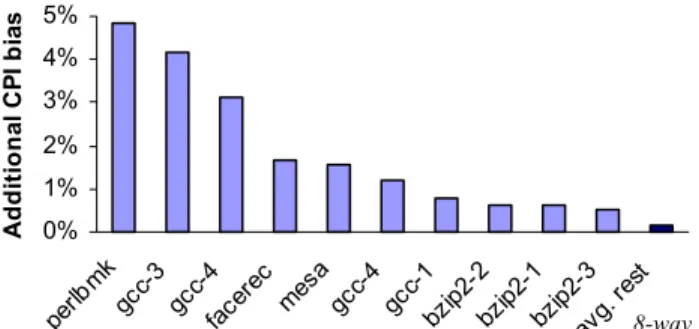
We evaluate MRRL with a reuse probability of 99.9% as recom-mended in [12]. This reuse probability results in an average of 4.1 million instructions of warming prior to each detailed window, which is 20% of the average full warming interval (20.5 million instruc-tions). Thus, an approximation for the runtime of the adaptive warming strategy is 20% of the functional warming time of SMARTS, plus detailed simulation time, or about 1.5 hours on average per benchmark (8-way).
We present the results of our accuracy evaluation of adaptive warming with MRRL for small windows in Figure 4. Both average (1.1%) and worst-case error (5.4%) are considerably worse than full warming (0.6% on average; 1.6% worst-case). Error is high because short detailed windows are sensitive to accurate cache state. MRRL does not allow detailed windows to be simulated indepen-dently because cache state must be stitched [18] between consecutive windows. To obtain low bias, detailed windows must be simulated in program order, precluding parallelization and online result reporting (see Section 6). If MRRL is used without stitched state (thereby assuming an empty cache at the start of each functional warming period) we observe a considerably higher CPI bias of 1.9% on aver-age, with a worst case of 11%.
Because of the high worst-case error and relatively modest speedup of adaptive warming, we do not choose adaptive warming to imple-ment live-points. Increasing warming over MRRL (or increasing the MRRL reuse probability threshold) will improve accuracy, but further reduces the speed of adaptive warming.
4.3 Checkpointed warming
The key concern in evaluating checkpointed warming is the reusabil-ity of a set of checkpoints across a series of experiments. Because checkpointed warming uses a full-warming simulation to generate microarchitectural state for large structures, its accuracy is identical to full warming. When the generated live-points can be used for at least two experiments, checkpointed warming provides a net speed gain over full warming.
To maximize the reusability of live-points, we wish to place as few constraints as possible on microarchitectural configuration. Check-pointed warming dynamically reconstructs the vast majority of microarchitectural structures (e.g., queues, ROB, etc.) through detailed warming. As such, the configurations of these dynamically-warmed structures are not constrained. For the remaining few
struc-tures, for which detailed warming requirements are large or cannot be determined (e.g., caches and branch predictors), we store a represen-tation of the structure in each point. The reusability of a live-point library is limited by the flexibility of these representations. There are two basic approaches to increasing live-point reusability. First, we can collect state snapshots for multiple component configu-rations in a single creation pass. The second, preferable approach is to modify the saved representation such that a range of organizations can be reconstructed when a live-point is loaded. However, we cannot easily apply this adaptable approach to some structures, such as modern branch predictors, and so we must store multiple warmed configurations. Cache-like structures, including the TLB, can typi-cally be stored using adaptable data structures.
Storing multiple configurations. The first approach is straight-forward and effective if the number of configurations of interest is relatively small. The major cost of live-point creation is the traversal of the entire benchmark instruction stream. Warming additional copies of a microarchitectural structure incurs a relatively small over-head. If the slowdown is less than a factor of two, it is a net win to collect state for both configurations in a single pass. We recommend this approach for storing branch predictor state.
Storing adaptable warmed state. With cache-like structures, it is possible to exploit the properties of cache replacement algorithms to create a representation of cache state from which one can accurately reconstruct a range of configurations [14]. Barr et al. propose a data structure, called the Memory Timestamp Record (MTR), that records the timestamp of the last access to each cache block during functional warming [1]. The MTR allows a simulator to reconstruct a cache hierarchy of arbitrary sizes and associativities assuming least-recently-used replacement and a lower bound on cache block size. Storing an MTR in each live-point enables reusability across nearly arbitrary cache hierarchy organizations, but incurs a storage cost proportional to the application’s memory footprint. However, researchers can often place an upper bound on the maximum cache size of interest. For a given maximum size and associativity, we can instead store a timestamp-sorted list of the most recent accesses mapping to each set, referred to as a Cache Set Record (CSR) by Barr et al. [1]. A CSR requires the same storage as the tag array for the selected maximum cache size, and allows reconstruction of all smaller and/or less associative caches.
Our analysis of simulation sampling warming methods demonstrates that checkpointed warming is both fast and accurate. The reusability weakness of checkpointed warming can be mitigated through careful planning of microarchitectural state representation. Thus, we choose to use checkpointed warming to implement live-points.
5. LIVE-POINTS WITH LIVE-STATE
Current publicly-available computer architecture simulators already provide a checkpoint creation and loading capability that allows the simulator to move to a particular program trace location in constant time [2,23]. These checkpoint implementations store only architec-turally-visible system state (i.e., memory, architectural register and peripheral device state). A straightforward approach to implement checkpointed warming is to extend these existing checkpoints with functionally-warmed microarchitectural state as described in Section 4.3. 0% 1% 2% 3% 4% 5% perlb mk gcc-3 gc c-4 facer ec mesagc c-4 gcc-1bzip2-2bzi p2-1 bzip2 -3 avg. r est A ddi ti ona l C P I bi as
Figure 4. Adaptive warming bias. Additional error is introduced by adaptive warming using MRRL vs. full warming.
Unfortunately, this straightforward approach is not practical because conventional checkpoints require prohibitive storage, proportional to the total memory footprint of an application (up to 200MB for SPEC2K [13]). We measured an average SPEC2K memory footprint of 105 MB. Thus, for SMARTS-like samples (~10,000 measurements), conventional checkpoints for all of SPEC2K require 33 TB of storage (7.2 TB with gzip compression). Sampling optimizations [9,28,36] reduce this cost by an order of magnitude at best. With these check-point sizes, simulations are I/O bound, and checkcheck-pointed warming can provide little, if any, speedup over functional warming. It may be possible to save space by storing only changes to memory between checkpoints, but this approach introduces dependence among check-points, precluding parallel simulation and other sampling optimiza-tions (see Section 6).
Reducing storage with live-state. We can drastically reduce check-point storage cost for live-check-points by storing only the state that will be accessed during the brief simulation window, an approach we call live-state. Because the detailed windows are just a few thousand instructions, only a tiny subset of state is accessed. Simulation state that is never referenced during measurement or detailed warming can be omitted from the checkpoint without affecting the simulation. The live-state approach stores the minimal set of accessed state for each live-point’s specified simulation window. Live-points can accu-rately simulate only the instructions within this pre-selected window. The restriction to a pre-selected window does not impact simulation sampling because the window locations and measurement/detailed warming periods are specified in advance by the sample design. We can identify precisely which instructions will commit during the selected window when we construct a live-point. Thus, it is straight-forward to identify all the memory and microarchitectural state these instructions will access—generally less than 32 KB per live-point (uncompressed, including ASN.1 encoding overhead).
However, we cannot identify the state that is accessed on non-committed speculative paths (wrong-path instructions). It is not possible to identify a priori the set of wrong-path instructions that will execute in all future simulations at live-point creation time. To do so requires either fixing all simulation parameters (queue sizes and latencies), or exploring all possible speculative paths to the depth they might be followed (as bounded by, for example, ROB size). The former eliminates checkpoint reusability, while the latter requires analysis that grows exponentially with speculation depth.
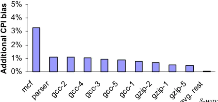
Effects of path instructions. Although the effects of wrong-path instructions on the commit instruction stream are generally small [3], they cannot be ignored given our tight bias goals. Errors in wrong-path modeling cause the schedule of wrong-path execution to differ from a simulation where all state is available, which in turn perturbs the execution schedule of the commit instruction stream. We measure the bias introduced if we restrict live-state to contain only state accessed by correct path instructions. With restricted live-state, we omit all architectural state (memory values) and microarchi-tectural state (cache tags and branch predictor entries) that are not accessed in the simulation window during live-point creation, leaving this state uninitialized (effectively random). A live-point with restricted live-state contains the smallest possible subset of state that can still simulate correct-path instructions (but will not accurately simulate wrong-path). Although the average bias increase for CPI is only 0.1%, the worst case is 3.3%. Figure 5 shows the bias results for the benchmarks with the most error.
Wrong-path instructions interact with the commit stream through resource contention and in the cache tag arrays. In the vast majority of cases, we can use branch predictor outcomes to identify the wrong-path instruction sequence, and cache tag arrays to identify wrong-path load latency. This information is sufficient to identify contention and cache tag array updates arising from speculative execution, without the need for the values accessed by wrong-path loads.
In our live-state approach, we include the microarchitectural state necessary to reflect wrong-path effects (branch predictor, cache tag arrays, TLBs), but omit memory values unless they are accessed on the correct-path. By omitting the vast majority of memory values, the live-state approach reduces storage requirements from over 100 MB to 142 KB per live-point (uncompressed; assuming cache hierarchy and branch predictor of our 8-way baseline). Under this approach, unavailable memory values enter the microarchitecture (via a wrong-path load) on average less frequently than once per detailed window. We measured no appreciable increase, < 0.1% difference, in CPI bias over full warming.
6. SAMPLING FRAMEWORK
One of the benefits of the live-point design is that each live-point is independent of all other live-points, and can thus be processed in isolation. As others have noted [10,19,21], window independence allows a simulation to be parallelized across hosts (with parallelism degree up to the sample size). However, we can also leverage live-point independence to minimize the runtime of absolute and compar-ative experiments, and provide results from simulations that are still in progress. The following subsections present a sampling methodol-ogy for absolute and comparative performance studies.
6.1 Absolute performance estimates
To report meaningful estimated results, a sampled simulation must complete processing of an unbiased sample of the complete bench-mark. With functional warming, where the measurements must be processed in strict program order, the measured sample represents the entire benchmark only after the entire simulation is complete. With independent live-points, we are not forced to process detailed windows in program order. We can exploit this property to rearrange the live-point processing order so that we can report unbiased perfor-mance estimates (with lower statistical confidence than final results) at any time. 0% 1% 2% 3% 4% 5% mcf parse r gc c-2 gc c-4 gcc-3 gcc-5gc c-1 gzip-2gz ip-1 gzi p-5 avg. r est A ddi ti ona l C P I bi as
Figure 5. Restricted live-state bias. If only correct-path state is stored, wrong-path instructions are not accurately simulated.
A complete live-point library forms an unbiased random (or system-atic) sample of a benchmark. If we select a random sub-sample from the live-point library, we arrive at a smaller, but still unbiased, random sample of the benchmark. Based on this principle, if we shuffle a live-point library into random order, after each live-point is simulated, the live-points processed thus far form an unbiased random sample of the benchmark.
We exploit random-order live-point processing to allow a simulation to report results at any time. As live-points are processed, we calcu-late the confidence achieved in the sample observed thus far. As the sample size grows, the confidence improves, and the estimated results converge to their true values. As soon as we are satisfied with the current confidence, we can terminate the simulation. We impose a minimum sample size of 30 live-points to ensure that the central limit theorem holds and our confidence calculations are valid [16]. Online monitoring of simulation results and their current confidence has proven valuable during simulator development to get quick-and-dirty performance estimates and detect simulator bugs. Even after processing a small sample (100’s of live-points), confidence intervals will be tight enough to identify gross performance bugs reliably. To maximize simulation processing speed, we recommend shuffling live-points on disk, prior to simulation. Live-points should be stored in a single compressed file to maximize I/O performance (which is the performance-limiting bottleneck in our environment).
6.2 Comparative performance estimates
When a live-point library is created, we set an upper bound on the sample size that can be measured with that library (i.e., the number of live-points in the library). The upper bound is typically based on the sample size required to meet a desired statistical confidence for a benchmark and baseline microarchitecture combination. Because the required sample size will increase when a new microarchitecture has higher target metric variability (e.g., CPI variance), a live-point library sized for the baseline configuration may fall short of the sample required for an experimental case.
In such comparative studies, researchers are often more interested in the relative performance of two designs than absolute performance. We can take advantage of this observation through a sampling proce-dure called matched-pair comparison, first proposed for computer architecture simulation sampling by Ekman and Stenström [9]. Matched-pair comparison exploits the phenomenon that the change in performance from design x to design y tends to vary less than the absolute performance of either design. As a result, the change in performance can be assessed to a given confidence with a smaller sample than absolute performance.
Under matched-pair comparison, we build a confidence interval directly on the change in performance. Unlike an unpaired compari-son of two different samples, in matched-pair comparicompari-son, we measure the same sample (i.e., same live-points) in each of two designs and compute the performance delta on each measurement interval. In the common case, the design change has a similar effect in all measurement intervals (e.g., a larger cache tends to improve performance uniformly by a small increment). Thus, the variance of the performance deltas, and required sample size, is small. The calcu-lations and procedure for applying matched-pair comparison are detailed fully in [9].
Ekman and Stenström report that matched-pair comparison typically reduces sample size by an order of magnitude compared to absolute performance estimates over a range of microarchitectural design changes. We performed a similar set of sensitivity studies (e.g., varying latencies, queue sizes, functional unit mix, etc.). Our results corroborate [9], indicating that matched-pair comparison reduces sample size by a factor of 3.5to 150. We note that matched-pair comparison is particularly effective for detecting that a design change has no appreciable impact (i.e., less than 3% CPI change). When a design change has little effect, nearly all measurement intervals behave identically under the base and experimental cases, resulting in low CPI-delta variance.
Matched-pair comparison addresses the risk that a comparative performance study will exhaust the available live-point library without achieving the desired confidence. If we size a live-point library such that it can achieve a particular confidence in an absolute estimate of the base case, we will typically require only a fraction of this library for comparative studies.
We can combine matched-pair comparison with random-order processing to report results online for comparative studies. The combined optimizations are particularly effective for rapidly search-ing a design space to eliminate designs that do not differ significantly from the base case. A 50-measurement sample can rapidly distin-guish design changes with no impact from those that require further simulation.
6.3 Experiment procedure
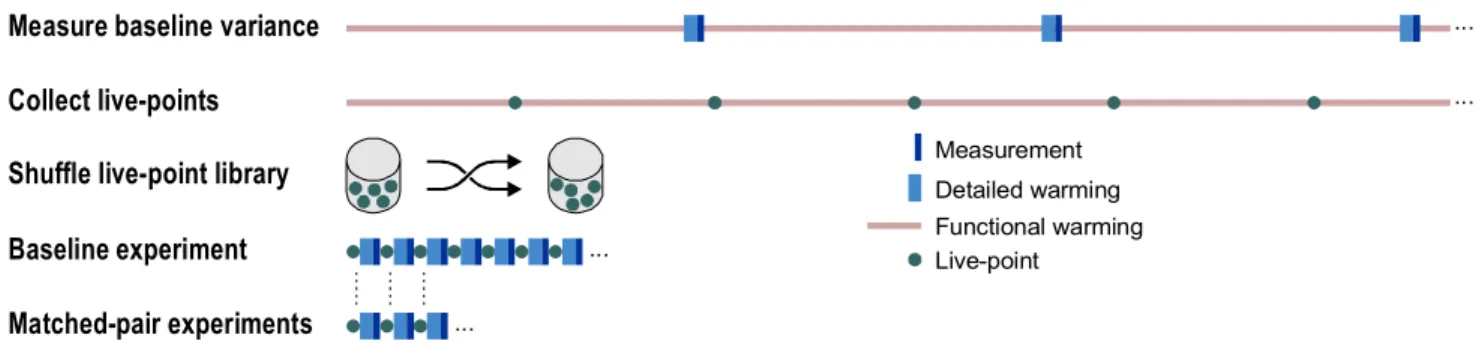
We now summarize our complete procedure for experimentation with live-points. Figure 6 illustrates the steps in the procedure.
First, we must measure the target metric variance for the baseline configuration to determine an appropriate live-point library size. We can measure variance using prior simulation sampling approaches, or estimate it from published results [37]. In our implementation, these simulations require seven hours on average for SPEC2K.
Collect live-points
Measure baseline variance
Baseline experiment
Matched-pair experiments
Shuffle live-point library
Functional warming Detailed warming Live-point Measurement ... ... ... ...
2.
1.
4.
5.
3.
Second, we must generate a live-point library. We choose the maximum cache hierarchy and set of branch predictors of interest, and run a full-warming simulation that outputs compressed live-points. Live-point generation requires on average 8.5 hours per benchmark.
Third, we shuffle these live-points into a random order and store them in a single compressed stream. Optionally, the live-point library can be split into multiple compressed streams for parallel processing. Shuffling is compression-speed bound, and requires several minutes per benchmark.
Fourth, we measure the baseline configuration with our live-point library. We record metrics of interest (e.g., CPI) for each live-point. This simulation can be parallelized and can employ the random-order processing optimization. For our 8-way microarchitecture, this simu-lation reaches 99.7% confidence of ±3% error in an average of 91 seconds per benchmark (without parallelization).
Finally, we can perform comparative studies relative to the baseline microarchitecture using the live-point library. These simulations can employ parallelization, random-order processing, and matched-pair comparison optimizations. Furthermore, we can monitor simulation results online, and terminate simulations at any time to report results with reduced confidence. If we assess our 16-way microarchitecture relative to our 8-way baseline, the simulation reaches target confi-dence in an average of 2.4 minutes per benchmark, while an absolute measurement of the 16-way microarchitecture requires 7.6 minutes per benchmark.
7. RESULTS
In this section, we report results on the effectiveness of the live-state approach in reducing storage cost and compare the performance of live-points to other simulation sampling approaches.
7.1 Live-state results
The live-state approach is highly effective at reducing the storage cost of live-points. Because the simulation window covered by each live-point is short (a few thousand instructions), only ~16 KB of memory state must be stored.
Live-state can also be used in conjunction with adaptive warming. However, because the simulation window required for cache warming is large (on average 4.1 million instructions per window), the required memory state is much larger, on average 360 KB.
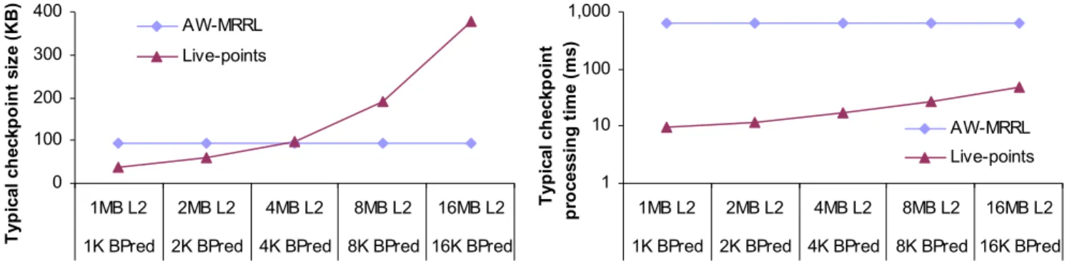
Figure 7 compares the uncompressed size of live-points (assumes cache/branch predictor of the 8-way microarchitecture) and live-state for adaptive warming using MRRL (AW-MRRL; microarchitecture independent). We typically obtain 5:1 compression with gzip. The storage cost (and thus decompression/load time) of live-points grows as the size of the stored microarchitectural structures increases. With adaptive warming, no microarchitecture-specific state is stored, and thus storage cost is fixed. As a result, there is a break-even point where the storage cost of live-points and adaptive warming become equal. Figure 8 (left) shows that this break-even threshold occurs around a 4 MB maximum cache size. However, for microarchitecture state larger than this threshold, live-points remain an order of magnitude faster (Figure 8 right) because generating cache state dynamically is much slower than loading it from disk.
7.2 Live-points performance
We use live-points to estimate the absolute CPI of our benchmark suite to the same accuracy and confidence as previous simulation sampling techniques as described in Section 3. Table 2 presents measured run-time results for live-points. Runtime results were collected with serial live-point processing and only a single simula-tion running per system. We compare live-points to non-sampled runs of the complete benchmark with SimpleScalar’s sim-outorder, full warming using SMARTSim [37], and adaptive warming using MRRL (AW-MRRL). We show the best, average, and worst runtimes for the two microarchitectural configurations intro-duced in Section 3.
Live-points eliminate the functional warming bottleneck in SMART -Sim, reducing average simulation time for SPEC2K benchmarks from 7 hours to just 1.5 minutes (8-way baseline microarchitecture). Live-points are 50 times faster than AW-MRRL. Live-point simula-tions often complete faster than native execution of benchmarks on
Register files, TLBs,
system call updates Branch predict or L1-D c ache ta gs L2 cac he tags Memory data L1-I ca che tag s 3 KB 363 KB 142 KB 3 KB 4 KB 8 KB 46 KB 64 KB 16 KB AW-MRRL Live-point 360 KB
Figure 7. Breakdown of a typical live-point (uncompressed). For comparison, a conventional checkpoint is 105 MB on average.
1 10 100 1,000
1MB L2 2MB L2 4MB L2 8MB L2 16MB L2 1K BPred 2K BPred 4K BPred 8K BPred 16K BPred
T yp ic al ch eck p o in t p ro ces si n g t im e (m s) AW-MRRL Live-points 0 100 200 300 400 1MB L2 2MB L2 4MB L2 8MB L2 16MB L2 1K BPred 2K BPred 4K BPred 8K BPred 16K BPred
T yp ical ch ec kp o in t s iz e ( K B ) AW-MRRL Live-points
Figure 8. Compressed checkpoint size and processing time. Live-points have a size advantage until large cache tag arrays are required. However, even for large caches, live-points are much faster than adaptive warming using MRRL because no functional warming is needed. 8-way
our host platform, which typically requires several minutes per benchmark.
For both SMARTSim and sim-outorder, simulation time varies linearly with benchmark length. Thus, we can expect simulation times to grow with longer benchmarks. In contrast, runtime with live-points and AW-MRRL depends on sample size, and thus CPI vari-ability. We do not observe any relationship between CPI variability and benchmark length; therefore, we do not expect live-points’ runt-imes to increase for longer benchmarks.
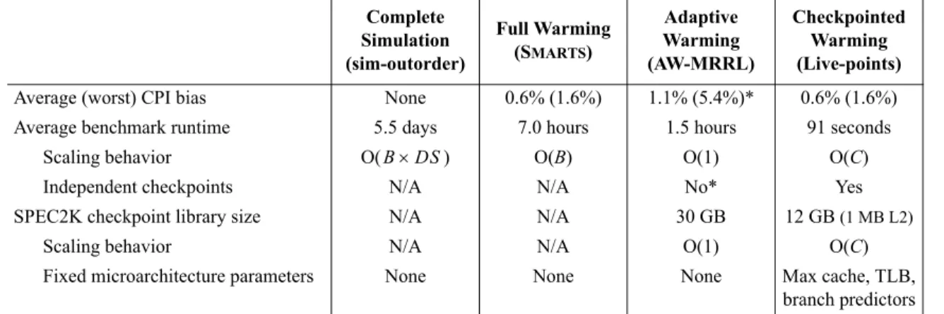
Table 3 summarizes the characteristics of the warming approaches evaluated in this paper. The table shows the live-point library sizes, run times, and biases measured for each technique.
Live-points match the bias of SMARTSim. AW-MRRL with a reuse distance threshold of 99.9% does not match this tight error. Adaptive warming accuracy may improve with a higher reuse threshold, at the cost of further slowdown relative to live-points. Sampling error can be made arbitrarily small with all three warming approaches by increasing sample size.
Table 3 also indicates the scaling behavior of live-point size and processing time with respect to microarchitectural model and bench-mark characteristics, and indicates what microarchitecture model parameters must be fixed when live-points are created. A live-point library restricts maximum cache and TLB sizes and must include state for each branch predictor used in subsequent simulations.
However, other microarchitectural configuration parameters are not fixed. Live-points are independent of one-another, enabling parallel simulation and online results reporting.
8. RELATED WORK
Many previous studies of simulation methodology present techniques orthogonal to our work. A variety of programming techniques can accelerate simulators by up to an order of magnitude without affect-ing simulation results [6,7,31]. However, simulation of complete benchmarks remains expensive. Construction and evaluation of short synthetic benchmarks with statistical properties similar to target workloads, commonly referred to as statistical simulation [24,25], can reduce simulation time to seconds. However, increasing the applicability, robustness and accuracy of these techniques remains an active research topic [8,17].
Ringenberg et al. [29] present intrinsic checkpointing, a checkpoint implementation that loads architectural state by instrumenting the simulated binary rather than through explicit simulator support. Unlike live-points, intrinsic checkpointing does not address microar-chitectural state.
Our work builds upon previous work on simulation sampling. Uniform simulation sampling was first proposed in the context of trace-based cache simulation [20]. Conte et al. proposed using sampling theory to calculate confidence of performance estimates Table 2. Runtimes of SPEC2K benchmarks. We include the fastest and slowest runtimes to show the variability of each technique.
8-way (1MB L2) 16-way (4MB L2)
Minimum Average Maximum Minimum Average Maximum
sim-outorder perlbmk2.2 h gcc-213 h 5.5 d mgrid15 d parser24 d perlbmk3.8 h gcc-222 h 9.6 d mgrid27 d parser42 d
SMARTSim perlbmk4.4 m gcc-229 m 7.0 h mgrid17 h parser25 h perlbmk4.6 m gcc-231 m 7.3 h mgrid18 h parser26 h
AW-MRRL perlbmk61 s eon-288 s 1.5 h ammp7.1 h parser9.5 h perlbmk65 s eon-292 s 1.6 h ammp7.5 h parser9.9 h
Live-points swim1 s eon-22 s 91 s 5.0 mvpr ammp12 m swim13 s eon-214 s 7.6 m 25 mvpr ammp1.3 h Times are specified in days (d), hours (h), minutes (m), or seconds (s).
Table 3. Summary of simulation sampling warming methods. Complete Simulation (sim-outorder) Full Warming (SMARTS) Adaptive Warming (AW-MRRL) Checkpointed Warming (Live-points) Average (worst) CPI bias None 0.6% (1.6%) 1.1% (5.4%)* 0.6% (1.6%) Average benchmark runtime 5.5 days 7.0 hours 1.5 hours 91 seconds
Scaling behavior O( ) O(B) O(1) O(C)
Independent checkpoints N/A N/A No* Yes
SPEC2K checkpoint library size N/A N/A 30 GB 12 GB (1 MB L2)
Scaling behavior N/A N/A O(1) O(C)
Fixed microarchitecture parameters None None None Max cache, TLB, branch predictors B DS×
B = benchmark length, C = max cache size, DS = detailed simulation speed
explicitly [5]. SMARTS [37] and similar recent work [22] minimize total instructions simulated in detail, and form the basis for our sampling methodology.
Other recent sampling proposals employ representative sampling [19,28,32]. In representative sampling, program phases are identified and a representative portion of each phase is measured. In contrast, all population elements have equal probability of inclusion in the sample under uniform sampling approaches.
The most prevalent representative sampling approach, SimPoint [28,32], identifies phases based on microarchitecture-independent analysis of the relative frequency of static basic blocks. Van Bies-brouck et al. [34] apply a checkpointed warming approach similar to live-points to accelerate SimPoint measurement. They report that checkpoint libraries for SimPoint-derived samples typically require less storage than high-confidence uniform samples (i.e., 99.7% confi-dence of ±3% error), whereas uniform samples simulate fewer instructions in detail per benchmark (~30 million rather than ~300 million instructions) and result in shorter simulation turn-around. Our experiments corroborate these results from this concur-rent work. However, with uniform sampling, we can reduce turnaround time and live-point storage cost at the cost of reduced confidence. Existing representative sampling techniques do not provide quantitative measures of confidence with each result [36], and provide only a single option for runtime, storage cost, and accu-racy. Moreover, online result reporting (see Section 6.1) is not appli-cable to representative sampling.
Live-points have been successfully integrated into the Liberty Simu-lation Environment (LSE) by researchers at Princeton University [27]. LSE is a computer architecture simulation infrastructure, which models microarchitecture at a structural, rather than behavioral, level of abstraction. As such, LSE models match hardware closely, but simulation is an order of magnitude slower than sim-outorder.
Integration of live-points into LSE reduced typical simulation times by up to 20x over SMARTS. Moreover, the online results reporting possible with live-points reduced the typical implement-debug-test cycle of model development to less than an hour, greatly accelerating the model development process.
9. CONCLUSION
Live-points reduce microarchitecture simulation time to the limit imposed by detailed simulation. We leverage state-of-the-art simula-tion sampling techniques to simulate a minimum of instrucsimula-tions in detail by using large sample sizes with small measurement intervals of 1000 instructions each. Unlike previous simulation sampling approaches, turnaround time with live-points is independent of benchmark length, depending only on the target metric’s variance. Therefore, live-points enable simulation of benchmarks far longer than those used currently, with no increase in simulation time. The live-state approach enables checkpointed warming with reasonable storage requirements by storing only necessary functionally-warmed state for several thousand instructions of accurate performance simu-lation. A reusable live-point library for SPEC2K requires only 12 GB. By processing live-points in a random order, our sampling framework allows simulations to report results while simulation is still in progress.
The vast increase in simulation speed possible with live-points trans-lates into a much higher experimental throughput. Parametric studies that cover a wide range of microarchitectural options can now be
evaluated accurately on entire benchmark suites with reasonable computational requirements. In addition, live-points enable interac-tive performance estimates for individual benchmarks in minutes, enabling quick evaluations of design decisions with immediate performance feedback.
10. REFERENCES
[1] K. C. Barr, H. Pan, M. Zhang, and K. Asanovic. Accelerating multiprocessor simulation with a memory timestamp record. In Proceedings of the International Symposium on Performance Analysis of Systems and Software, Mar. 2005.
[2] D. Burger and T. M. Austin. The SimpleScalar tool set, version 2.0. Technical Report 1342, Computer Sciences Department, Uni-versity of Wisconsin–Madison, June 1997.
[3] H. W. Cain, K. M. Lepak, B. A. Schwartz, and M. H. Lipasti. Pre-cise and accurate processor simulation. In Workshop on Computer Architecture Evaluation using Commercial Workloads, HPCA, Feb. 2002.
[4] S. Chen. Direct smarts: Accelerating microarchitectural simula-tion through direct execusimula-tion. Master’s thesis, Carnegie Mellon University, May 2004.
[5] T. M. Conte, M. A. Hirsch, and K. N. Menezes. Reducing state loss for effective trace sampling of superscalar processors. In Pro-ceedings of the International Conference on Computer Design, Oct. 1996.
[6] M. Durbhakula, V. S. Pai, and S. Adve. Improving the accuracy vs. speed tradeoff for simulating shared-memory multprocessors with ILP processors. In Proceedings of the International Sympo-sium on High-Performance Computer Architecture, Jan. 1999. [7] S. Dwarkadas, J. R. Jump, and J. B. Sinclair. Execution-driven
simulation of multiprocessors: Address and timing analysis. IEEE Transactions on Modeling and Computer Simulation, Volume 4, No. 4:314–338, Oct. 1994.
[8] L. Eeckhout, R. B. Jr., B. Stougie, K. D. Bosschere, and L. K. John. Control flow modeling in statistical simulation for accurate and efficient processor design studies. In Proceedings of the Inter-national Symposium on Computer Architecture, June 2004. [9] M. Ekman and P. Stenstrom. Enhancing multiprocessor
architec-ture simulation speed using matched-pair comparison. In Pro-ceedings of the International Symposium on Performance Analysis of Systems and Software, Mar. 2005.
[10] S. Girbal, G. Mouchard, A. Cohen, and O. Temam. DiST: a sim-ple, reliable and scalable method to significantly reduce processor architecture simulation time. In Proceedings of the International Conference on Measurement and Modeling of Computer Systems, June 2003.
[11] N. Hardavellas, S. Somogyi, T. F. Wenisch, R. E. Wunderlich, S. Chen, J. Kim, B. Falsafi, J. C. Hoe, and A. G. Nowatzyk. Sim-flex: A fast, accurate, flexible full-system simulation framework for performance evaluation of server architecture. SIGMETRICS Performance Evaluation Review, May 2004.
[12] J. W. Haskins and K. Skadron. Memory reference reuse latency: Accelerated warmup for sampled microarchitecture simulation. In Proceedings of the International Symposium on Performance Analysis of Systems and Software, Mar. 2003.
[13] J. L. Henning. SPEC CPU2000: Measuring CPU performance in the new millennium. Computer, 33(7):28–35, 2000.
[14] M. D. Hill and A. J. Smith. Evaluating associativity in cpu cach-es. IEEE Transactions on Computers, C-38(12):1612–1630, Dec. 1989.
[15] International Organization for Standardization. ASN.1 encoding rules: Specification of Basic Encoding Rules (BER), Canonical Encoding Rules (CER) and Distinguished Encoding Rules (DER). ISO/IEC 8825-1:2002 | ITU-T Rec. X.690 (2002).
[16] R. K. Jain. The art of computer systems performance analysis: Techniques for experimental design, measurement, simulation, and modeling. Wiley, 2001.
[17] R. B. Jr., L. Eeckhout, and L. K. John. Debunking statistical sim-ulation in HLS. In Proceedings of the Workshop on Duplicating, Deconstructing, and Debunking, June 2004.
[18] R. E. Kessler, M. D. Hill, and D. A. Wood. A comparison of trace-sampling techniques for multi-megabyte caches. IEEE Transactions on Computers, 43(6):664–675, June 1994. [19] T. Lafage and A. Seznec. Choosing representative slices of
pro-gram execution for microarchitecture simulations: A preliminary application to the data stream. In IEEE Workshop on Workload Characterization, ICCD, Sept. 2000.
[20] S. Laha, J. H. Patel, and R. K. Iyer. Accurate low-cost methods for performance evaluation of cache memory systems. IEEE Transactions on Computers, Volume C-37(11):1325–1336, Feb. 1988.
[21] G. Lauterbach. Accelerating architectural simulation by parallel execution of trace samples. In Hawaii International Conference on System Sciences, volume Volume 1: Architecture, pages 205– 210, Jan. 1994.
[22] W. Liu and M. Huang. Expert: Expedited simulation exploiting program behavior repetition. In Proceedings of the International Conference on Supercomputing, June 2004.
[23] P. S. Magnusson, M. Christensson, J. Eskilson, D. Forsgren, G. Hallberg, J. Hogberg, F. Larsson, A. Moestedt, and B. Werner. Simics: A full system simulation platform. IEEE Computer, 35(2):50–58, Feb. 2002.
[24] S. Nussbaum and J. E. Smith. Modeling superscalar processors via statistical simulation. In Proceedings of the International Con-ference on Parallel Architectures and Compilation Techniques, Sept. 2001.
[25] M. Oskin, F. T. Chong, and M. K. Farrens. HLS: combining sta-tistical and symbolic simulation to guide microprocessor designs. In Proceedings of the International Symposium on Computer Ar-chitecture, June 2000.
[26] V. S. Pai, P. Ranganathan, and S. V. Adve. The impact of in-struction-level parallelism on multiprocessors performance and simulation methodology. In Proceedings of the Third IEEE Sym-posium on High-Performance Computer Architecture, pages 72–
83, February 1997.
[27] D. A. Penry, M. Vachharajani, and D. I. August. Rapid develop-ment of flexible validated processor models. Technical Report 04-03, Princeton, Nov. 2004.
[28] E. Perelman, G. Hamerly, and B. Calder. Picking statistically valid and early simulation points. In Proceedings of the Interna-tional Conference on Parallel Architectures and Compilation Techniques, Sept. 2003.
[29] J. Ringenberg, C. Peloski, D. Oehmke, and T. Mudge. Intrinsic Checkpointing: A methodology for decreasing simulation time through binary modification. In Proceedings of the International Symposium on Performance Analysis of Systems and Software, Mar. 2005.
[30] M. Rosenblum, S. A. Herrod, E. Witchell, and A. Gupta. Com-plete computer simulation: The simos approach. IEEE Parallel and Distributed Technology, 1995.
[31] E. Schnarr and J. Larus. Fast out-of-order processor simulation using memoization. In Proceedings of the International Confer-ence on Architectural Support for Programming Languages and Operating Systems, Oct. 1998.
[32] T. Sherwood, E. Perelman, G. Hamerly, and B. Calder. Auto-matically characterizing large scale program behavior. In Pro-ceedings of the Tenth International Conference on Architectural Support for Programming Languages and Operating Systems, Oct. 2002.
[33] Standard Performance Evaluation Corporation. SPEC CPU2006 submission requirements. http://www.spec.org/cpu2006/, 2006. [34] M. Van Biesbrouck, L. Eeckhout, and B. Calder. Efficient
sam-pling startup for sampled processor simulation. In International Conference on High Performance Embedded Architectures & Compilers, Nov. 2005.
[35] M. Van Biesbrouck, T. Sherwood, and B. Calder. A co-phase matrix to guide simultaneous multithreading simulation. In Pro-ceedings of the International Symposium on Performance Analy-sis of Systems and Software, June 2004.
[36] R. E. Wunderlich, T. F. Wenisch, B. Falsafi, and J. Hoe. An eval-uation of stratified sampling of microarchitecture simulations. In Workshop on Duplicating, Deconstructing, and Debunking, IS-CA, June 2004.
[37] R. E. Wunderlich, T. F. Wenisch, B. Falsafi, and J. C. Hoe. Smarts: Accelerating microarchitecture simulation via rigorous statistical sampling. In Proceedings of the International Sympo-sium on Computer Architecture, June 2003.
[38] J. J. Yi, D. J. Lilja, R. Sendag, S. V. Kodakara, and D. M. Hawk-ins. Characterizing and comparing prevailing simulation method-ologies. In Proceedings of the International Symposium on High-Performance Computer Architecture, Feb. 2005.