INTL JOURNAL OF ELECTRONICS AND TELECOMMUNICATIONS, 2016, VOL. 62, NO. 4, PP. 401-408 Manuscript received April 19, 2016; revised November, 2016. DOI: 10.1515/eletel-2016-0055
Abstract— The main aim of this paper is to propose Cubic
Spline-Quantum Neural Network (CS-QNN) model for analysis and classification of Electroencephalogram (EEG) signals. Experimental data used here were taken from seven different electrodes. The work has been done in three stages, normalization of the signals, extracting the features by Cubic Spline Technique (CST) and classification using Quantum Neural Network (QNN). The simulation results showed that five types of EEG signals were classified with an average accuracy for seven electrodes that is 94.3% when training 70% of the features while with an average accuracy of 92.84% when training 50% of the features.
Keywords—EEG Signals, ERP Signals, Cubic Spline, Neural
Networks, Quantum Neural Networks
I. INTRODUCTION
HE biomedical engineering interested dramatically in the automatic classification of Electroencephalogram (EEG) signals. Because the biomedical signals, inherently unstable and randomly change over time depending on the change and mental health conditions and situations of tension for the same person, and one of these signals is brain signal that varies according to the psychological state of the person himself and changed depending on the circumstances, all of this has paid great attention to the analysis of brain signals. The EEG is the registration of electrical activity on the scalp. Current flow due to firing of nerve cells in the brain results in a voltage wiggle that measured as EEG [1]. Measuring the brain's response to a stimulus is called event-related potential (ERP). The stimulus can be motor, sensory, or cognitive naturally. Human ERPs are usually recorded from electrodes placed on the human scalp.
Fig. 1. The placement of electrodes on the scalp according to the international (10-20) standard.
Authors are with University of Babylon, College of Engineering, Electrical Engineering Department, Iraq (email: {ehabalhialy; mariam.raheem} @yahoo.com).
The placement of electrodes on the scalp according to the international (10-20) standard is shown in fig. 1 [2]. The popular way of analyzing event-related EEG signals is the computation of ERPs. This can be done by repeating an event of interest such as a visual stimulus of a computer screen and analyzing a small fraction of the EEG activity that is evoked by this event [3]. The feature extraction technique of EEG signals provides an accurate features in which would to classify between any event-related potentials of the brain using QNN. Five types of EEG signals are used. Each type of these signals is a mental task assigned to a particular person to perform it. These tasks are (baseline, multiplication, letter composing, rotation, counting).
II. FEATURE EXTRACTION AND SELECTION
A feature is a distinct or characteristic measurement, change, basic component that can extract from a slice of a signal. The features used to represent the signals without losing the important information about these signals. The feature extraction process is the determination of the feature or the feature vector from the signal. So as to make signal processing problems can be solved, need to convert signals to features which will become abbreviated representations of the signals, which only contain important information for the signal. The aim of this section is to identify convenient input feature vectors which would discriminate between the event-related potentials of the brain. In this work, EEG signal analysis is divided into five parts: normalization, knot extraction, knot selection, feature extraction and classifier.
A. Normalization
The normalization is a process of removing, the difference in the amplitude between the signals in each kind or category. In order to make the data has a zero mean; the computed mean of data will be subtracted from the raw EEG signal. Normalization steps can be summarized as follows:
1. For EEG signals, mean value of data is stable to zero value. Thus, the offset will be removed from the signal. 2. Subtract the mean value from the raw EEG signal. 3. After subtraction, the mean value of the original EEG
signal, must be zero or nearby zero.
B.
Knot extraction
The accurate analyses of the EEG signal have special importance in this system. Where extract the features of the EEG signal depends firstly and dramatically on determining characteristic points sites, whenever these sites were accurate,
Classification of EEG Signals Using Quantum
Neural Network and Cubic Spline
Mariam Abdul-Zahra Raheem and Ehab AbdulRazzaq Hussein
the extracted features of the signals were accurate too. A technique that is used to find the knots largely depended on the shape of the EEG signal. These knots which are a part of the data can found by sorting data in ascending order after the data is divided into many parts and then to find the upper and lower values in every part of the data parts. This process will be repeated multiple times and in every time the number of the extracted knots will be increasing and will be saved in a matrix and will remove the duplicate points meaning that knots formerly extracted will be removed in order to prevent repetition.
C. Knot Selection
The extracted knots may not represent significant changes in the signal, or may be convergent between values, so that, in order to solve this problem, each extracted knots will be considered as a new data and will insert into the same technique previously used and thus will get only the distinctive knots that represent significant changes of the signal and will delete excess of the knots (the last knots) without losing the basic information of the signal.
D. Feature extraction using Cubic Spline Technique
Cubic spline interpolation is a useful technique to interpolate between known data points due to its stable and smooth characteristics [4]. The objective of the cubic spline interpolation is to get an interpolation formula, which is continuous in both first and second derivatives, both inside the intervals and at the interpolating knots. This will give function interpolation more smoothly. Generally, if the function to be approximate was smooth, then the cubic splines will do what is better than the piecewise linear interpolation [5].
The function S that consists of n-1 cubic polynomial pieces will be constructed as:
𝑆(𝑥) = { 𝑠1(𝑥) 𝑠2(𝑥) 𝑠𝑛−1(𝑥) 𝑖𝑓 𝑖𝑓 ⋮ 𝑖𝑓 𝑥1 𝑥2 𝑥𝑛−1 ≤ ≤ ≤ 𝑥 𝑥 𝑥 < < < 𝑥2 𝑥3 𝑥𝑛−1 (1)
Where Sᵢ is a third degree polynomial defined by:
𝑆ᵢ(𝑥) = 𝑎ᵢ(𝑥 − 𝑥ᵢ)3+ 𝑏ᵢ(𝑥 − 𝑥ᵢ)2− 𝑐ᵢ(𝑥 − 𝑥ᵢ) + 𝑑ᵢ (2)
Where n is the number of extracted knots. The cubic spline will need to conform to the following stipulations [6]:
1. The piecewise function 𝑆(𝑥) will interpolate all knots. 2. 𝑆(𝑥) will be continually on the interval [x₁,xn]. 3. 𝑆′(𝑥) will be continually on the interval [x₁,xn ]. 4. 𝑆′′(𝑥) will be continually on the interval [x₁,xn].
As the piecewise function 𝑆(𝑥) will interpolate all of the knots, we can conclude that [7]:
𝑆(𝑥ᵢ) = 𝑦ᵢ (3) For i = 1, 2, ..., n-1. Since 𝑥ᵢ 𝜖 [𝑥ᵢ, 𝑥ᵢ₊₁]
𝑆(𝑥ᵢ) = 𝑠ᵢ(𝑥ᵢ) (4) The mathematical expression for Natural Cubic Spline (NCS)
condition is:
𝑆′′(𝑥₁) = 𝑆′′(𝑥n) (5) Two additional conditions are needed to determine the natural
cubic splines which they are 𝑒₁ = 𝑒𝑛= 0 for every subinterval
[xi, xi+1] and the other values of 𝑒ᵢ were not yet known. Then the curvatures are linear in an interval and denoting values at the points 𝑥ᵢ as:
𝑒𝑖= 𝑠ᵢ′′(𝑥ᵢ), 𝑖 = 1,2, … , 𝑛. (6)
They comprise a linear spline for the data set (𝑥ᵢ , 𝑒ᵢ , 𝑖 = 1,2, … , 𝑛) therefore: 𝑠 (𝑥) = 𝑒𝑖+1 𝑥−𝑥𝑖 𝑥𝑖+1−𝑥𝑖+ 𝑒𝑖 𝑖 ′′ 𝑥𝑖+1−𝑥 𝑥𝑖+1−𝑥𝑖, 𝑖 = 1,2, … . , 𝑛 − 1 (7)
By integrating over x twice, will get:
𝑠𝑖(𝑥) = 𝑒𝑖+1 6ℎ𝑖 (𝑥 − 𝑥𝑖) 3+ 𝑒𝑖 6ℎ𝑖(𝑥𝑖+1− 𝑥) 3+ 𝑐(𝑥 − 𝑥 𝑖) + 𝑑(𝑥𝑖+1− 𝑥) (8) Where ℎ𝑖= 𝑥𝑖−1− 𝑥𝑖. (9)
And c and d are constants of integration. The terms of interpolation 𝑠𝑖(𝑥𝑖) = 𝑦𝑖 And 𝑠𝑖+1(𝑥𝑖+1) = 𝑦𝑖+1 𝑒𝑖 6ℎ𝑖(𝑥𝑖+1− 𝑥) 3+ 𝑑(𝑥 𝑖+1− 𝑥) = 𝑦𝑖 (10) And 𝑒𝑖+1 6ℎ𝑖 (𝑥𝑖+1− 𝑥) 3+ 𝑐(𝑥 𝑖+1− 𝑥) = 𝑦𝑖+1 (11)
Applying the C0 conditions, will get:
𝑐 =𝑦𝑖+1 ℎ𝑖 − 𝑒𝑖+1ℎ𝑖 6 ; 𝑑 = 𝑦𝑖 ℎ𝑖− 𝑒𝑖ℎ𝑖 6 (12)
From the C1 continuity condition, the other values of 𝑒
𝑖 can be
found and by differentiating equation (8) after compensating c
& d, will get:
𝑠𝑖′(𝑥) = 𝑒𝑖+1 2ℎ𝑖 (𝑥 − 𝑥𝑖) 2− 𝑒𝑖 2ℎ𝑖(𝑥𝑖+1− 𝑥) 2+ (𝑦𝑖+1 ℎ𝑖 − 𝑒𝑖+1ℎ𝑖 6 ) − (𝑦𝑖 ℎ𝑖− 𝑒𝑖ℎ𝑖 6 ) (13) And 𝑠𝑖′(𝑥𝑖) = − 𝑒𝑖 2ℎ𝑖ℎ𝑖 2 + (𝑦𝑖+1 ℎ𝑖 − 𝑒𝑖+1ℎ𝑖 6 ) − ( 𝑦𝑖 ℎ𝑖− 𝑒𝑖ℎ𝑖 6 ) (14) 𝑠𝑖′(𝑥𝑖) = − 𝑒𝑖+1ℎ𝑖 6 − 𝑒𝑖ℎ𝑖 3 + 𝑏𝑖 (15) Where 𝑏𝑖= 𝑦𝑖+1−𝑦𝑖 ℎ𝑖 , 𝑖 = 1,2, … , 𝑛 − 1 (16) Also 𝑠𝑖−1′ (𝑥𝑖) = 𝑒𝑖 2ℎ𝑖−1ℎ𝑖−1 2 + ( 𝑦𝑖 ℎ𝑖−1− 𝑒𝑖ℎ𝑖−1 6 ) − ( 𝑦𝑖−1 ℎ𝑖−1− 𝑒𝑖−1ℎ𝑖−1 6 ) = 𝑒𝑖−1ℎ𝑖−1 6 + 𝑒𝑖ℎ𝑖−1 3 + 𝑏𝑖−1 (17) 𝑠𝑖−1′ (𝑥𝑖) = 𝑠𝑖′(𝑥𝑖) (18)
By setting equation (18) at all interior points, will obtain:
ℎ𝑖−1𝑒𝑖−1+ 2(ℎ𝑖−1+ ℎ𝑖)𝑒𝑖+ ℎ𝑖𝑒𝑖+1= 6(𝑏𝑖− 𝑏𝑖−1) (19)
Which is a tridiagonal system of equations in terms of the unknowns 𝑒𝑖's. There are 𝑛 unknowns and 𝑛 − 2 equations.
These equations can be rearranged as:
𝑒1= 0 ℎ𝑖−1𝑒𝑖−1+ 𝑢𝑖𝑒𝑖+ ℎ𝑖𝑒𝑖+1= 𝑣𝑖 𝑖 = 2,3, … , 𝑛 − 1 (20) 𝑒𝑛= 0 Where 𝑢𝑖= 2(ℎ𝑖−1+ ℎ𝑖) (21) 𝑣𝑖= 6(𝑏𝑖− 𝑏𝑖−1), 𝑖 = 2,3, … , 𝑛 − 1 (22)
By using the tridiagonal solver, the values of (𝑒2, 𝑒3, … 𝑒𝑛)
can be obtained. These values in addition to 𝑒1= 𝑒𝑛= 0 can
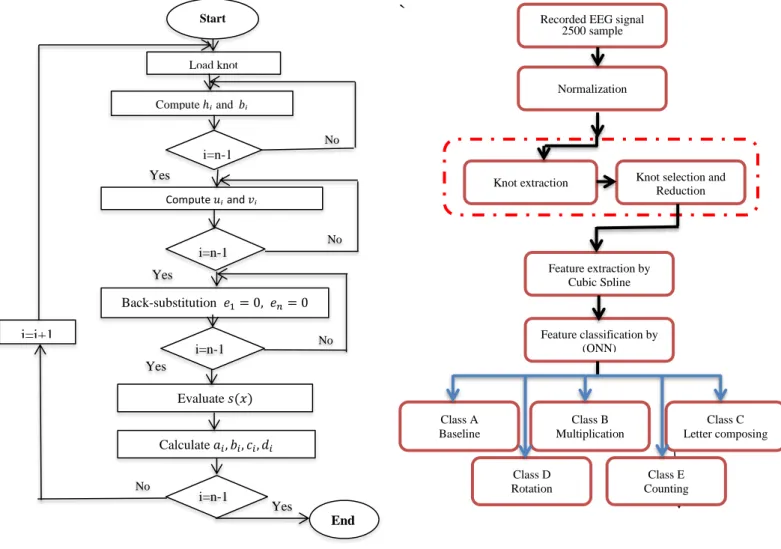
then be used to find out the splines by the compensation in equation (8). Figure 2 shows the flowchart of cubic spline technique.
The cubic spline technique approach has many steps can be described as follows:
1. The extracted knot for each signal of EEG signals is considered as interpolation points of the cubic spline.
CLASSIFICATION OF EEG SIGNALS USING QUANTUM NEURAL NETWORK AND CUBIC SPLINE 403
Fig. 2. Flowchart of CST approach.
2. Forty coefficients are extracted for each beat and these coefficients are rotated to represent one column.
3. Between each neighboring two knots, four coefficients (features) are extracted representing the coefficients of the third degree equation.
III. EEG SIGNAL CLASSIFICATION SYSTEM
PROPOSED
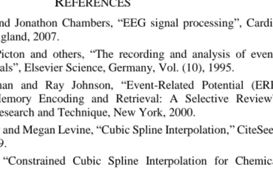
The main goal of the proposed system is to analyze the EEG signals depending on the cubic spline as a different way to extract the features of the signals and use QNN for classification. Figure 3 shows the general schematic diagram of the proposed system. Every one signal of EEG signals is formed by 2500 samples, which represents a vector pattern. These vectors in the data set will be normalized. After normalization, knots are extracted and then select the best knot, that is represents the basic characteristics of EEG signal form and its distinctive points. By cubic spline algorithm, the features have been extracted based on these knots. And then after forming the feature vectors, they will be applied to the QNN for classification or training purposes.A three layers (L) QNN used as a classifier for EEG signal, which is use the extracted features obtained by CST for training and testing purposes. The training process was conducted until reached a maximum iteration. QNN contains (5) output neurons (no) in the output layer, (40) input
neurons (ni) in the input layer.
`
Fig. 3. Structure of EEG Classification System.
IV. QUANTUM NEURAL NETWORK
Quantum Neural Network (QNN) is an energetic science based on the combination of quantum computing and artificial neural network. It also combines the benefits of fuzzy theoretic principles and neural modelling. Are similar to classical neural networks, QNNs has an inherently fuzzy architecture that can degrade the sample information to discrete levels of certainty or uncertainty. The transfer functions of quantum neuron able to form graded sections instead of crisp linear sections of the feature space. If the feature vectors lie at the boundary between interlaced classes, QNN will assign it partly to all related classes. If no certainty exists, QNN will assign it to the corresponding class [8].
The back-propagation algorithm used to modify the parameters for the desired output. The procedures of the algorithm are the error at the output layer which spread backward down to the input layer passing the hidden layer in the network in order to get the final desired outputs. The gradient descent method is utilized to calculate the phase variable 𝜃𝑗𝑠
and phase controlled factor 𝑑𝑤𝑖𝑘of the network and adjusts
them to minimize the output error [9].
V. LEARNING ALGORITHM FOR THE QNN
The gradient descent method is used to train the QNN of multi-layer excitation function. In each training cycle, the training algorithm revises both the connection weight between Start Load knot Back-substitution 𝑒1= 0, 𝑒𝑛= 0 Evaluate𝑠(𝑥) Calculate𝑎𝑖, 𝑏𝑖, 𝑐𝑖, 𝑑𝑖 End No Compute 𝑢𝑖 and 𝑣𝑖 Yes No Yes No Yes Yes No i=i+1 i=n-1 i=n-1 i=n-1 Compute ℎ𝑖and 𝑏𝑖 i=n-1
Recorded EEG signal 2500 sample
Normalization
Knot selection and Reduction Knot extraction Feature extraction by Cubic Spline Feature classification by (QNN) Class E Counting Class A Baseline Class D Rotation Class B Multiplication Class C Letter composing
the different level neuron and quantum intervals of the hidden layer [10].
There are two steps to train the QNN. The first step is making the input sample data compatible with the relevant class spaces by updating the connecting weights. The second step is embodying the uncertainty of data by updating the quantum intervals of quantum neurons in the hidden layer [11].
A. Update the synaptic weights in QNN
First should train the weights which involve presenting all the training set to the network and a forward pass and back propagation like a normal neural network. Let 𝑑𝑘 =
[𝑑1𝑘𝑑2𝑘𝑑3𝑘… 𝑑𝑛𝑜
𝑘 ]𝑇 be the desired output vector for the 𝑥𝑘
input feature vector 𝑥𝑘 = [𝑥
1𝑘, 𝑥2𝑘, 𝑥3𝑘, … , 𝑥𝑛𝑖
𝑘]𝑇. Let 𝑦 𝑖𝑘 =
[𝑦1𝑘𝑦2𝑘𝑦3𝑘… 𝑦𝑛𝑘𝑜]𝑇 be the actual output [12]. A gradient descent
based algorithm for learning the synaptic weights of the QNN can be derived by minimizing the quadratic error function sequentially for each 𝑘.
𝐸𝑘=1
2∑ (𝑑𝑖
𝑘 𝑛𝑜
𝑖=1 − 𝑦𝑖𝑘)2 𝑘 = 1,2, … , 𝑚 (23)
Where E: mean square error functions, 𝑚 is the total number of the training pattern. The synaptic weights are adjusted so as to minimize this error. This can be accomplished by adjusting or changing each synaptic weight by an amount proportional to the gradient of 𝐸𝑘 with regard to this specific synaptic weight.
The process of weights updating starting with the initial guess of the weight (which may be selected at random) and then a series of weights are generated using the following formulas: This update could be found via calculate the derivative of E𝑘
with respect to 𝑤𝑗𝑖 as:
𝑤𝑗𝑖(𝑟 + 1) − 𝑤𝑗𝑖(𝑟) = −𝜂 ∂E𝑘 𝜕𝑤𝑗𝑖= 𝜂 ∑ (𝑑𝑖 𝑘 𝑛𝑜 𝑖=1 − 𝑦𝑖𝑘) ∂y𝑖𝑘 𝜕𝑤𝑗𝑖 (24)
Where 𝑤𝑗𝑖(𝑟 + 1)𝑎𝑛𝑑 𝑤𝑗𝑖(𝑟) are the values representing a 𝑤𝑗𝑖
after and before the modification for the 𝑘𝑡ℎ inputs and 𝜂 is a small positive number called the learning rate, 0 < 𝜂 < 1.
∂y𝑖𝑘 𝜕𝑤𝑗𝑖= 𝑦𝑖 𝑘′ 𝐻̌ 𝑗𝑘 (25) Where 𝑦𝑖𝑘 ′ = 𝛽𝑜𝑦𝑖𝑘(1 − 𝑦𝑖𝑘) (26) ∂E𝑘 𝜕𝑤𝑗𝑖= 𝛽𝑜𝑒𝑖 𝑘𝑦 𝑖𝑘(1 − 𝑦𝑖𝑘) 𝐻̌𝑗𝑘 (27)
Substituting equation (27) into equation (24), the update equation is obtained as:
𝑤𝑗𝑖(𝑟 + 1) − 𝑤𝑗𝑖(𝑟) = 𝜂𝛽𝑜𝑒𝑖𝑘𝑦𝑖𝑘(1 − 𝑦𝑖𝑘) 𝐻̌𝑗𝑘 (28)
Since
𝑤𝑗𝑖(𝑟 + 1) = 𝑤𝑗𝑖(𝑟) − 𝜂𝑑𝑤𝑖𝑘∗ 𝐻̌𝑗𝑘 (29)
Where
𝑑𝑤𝑖𝑘= 𝛽𝑜𝑒𝑖𝑘𝑦𝑖𝑘(1 − 𝑦𝑖𝑘) , 𝑒𝑖𝑘=𝑑𝑖𝑘− 𝑦𝑖𝑘 , 𝐻̌𝑗𝑘 is the output of
the 𝔧𝑡ℎ hidden neuron.
For synaptic weight v𝑙𝑗 that connecting between the 𝑗𝑡ℎ hidden
unit and the 𝑘𝑡ℎ input unit, the update equation will be derived:
v𝑙𝑗(𝑟 + 1) − v𝑙𝑗(𝑟) = −𝜂 ∂E𝑘 𝜕𝑣𝑙𝑗= 𝜂 ∑ (𝑑𝑖 𝑘 𝑛𝑜 𝑖=1 − 𝑦𝑖𝑘) ∂y𝑖𝑘 𝜕𝑣𝑗𝑖 (30)
Where v𝑙𝑗(𝑟 + 1) and v𝑙𝑗(𝑟) are the values of v𝑙𝑗 before and
after the adaptation.
∂y𝑖𝑘 𝜕𝑣𝑗𝑖= 𝑦𝑖 𝑘′∑ 𝑤 𝑗𝑖 𝑛𝑜 𝑖=1 𝐻̌𝑗𝑘 𝜕𝑣𝑗𝑖 (31) With 𝑦𝑖𝑘 ′
as defined in equation (26), the definition of 𝐻̌𝑗𝑘
is: 𝐻̌𝑗𝑘 𝜕𝑣𝑗𝑖= 𝛽ℎ 1 𝑛𝑠∑ ℎ𝑗 𝑠,𝑘 𝑛𝑠 𝑠=1 (1 − ℎ𝑗 𝑠,𝑘)𝑥 𝑙 𝑘 (32)
Substituting equation (31) and equation (32) in equation (30), the update equation becomes:
∂E𝑘 𝜕𝑣𝑙𝑗= 𝛽ℎ𝛽𝑜∑ 𝑒𝑖 𝑘𝑦 𝑖𝑘(1 − 𝑦𝑖𝑘) 𝑛𝑜 𝑖=1 𝑤𝑗𝑖 1 𝑛𝑠∑ ℎ𝑗 𝑠,𝑘 𝑛𝑠 𝑠=1 (1 − ℎ𝑗 𝑠,𝑘)𝑥 𝑙𝑘 (33) Result: v𝑙𝑗(𝑟 + 1) − v𝑙𝑗(𝑟) = 𝜂 ∑ 𝑑𝑤𝑖𝑘 𝑛𝑜 𝑖=1 𝑤𝑗𝑖 1 𝑛𝑠∑ ℎ𝑗 𝑠,𝑘 𝑛𝑠 𝑠=1 (1 − ℎ𝑗𝑠,𝑘) ∗ 𝛽ℎ 𝑥𝑙𝑘 (34) Since v𝑙𝑗(𝑟 + 1) − v𝑙𝑗(𝑟) = 𝜂𝑑𝑣𝑖𝑘∗ 𝛽ℎ 𝑥𝑙𝑘 (35) Where 𝑑𝑣𝑖𝑘= ∑ 𝑑𝑤𝑖𝑘 𝑛𝑜 𝑖=1 𝑤𝑗𝑖 1 𝑛𝑠∑ ℎ𝑗 𝑠,𝑘 𝑛𝑠 𝑠=1 (1 − ℎ𝑗 𝑠,𝑘) (36)
B. Updating the quantum intervals
First, QNN must be trained in order to recognize transitions occurring between classes. The synaptic weights of the QNN must be updated to enable the network to learn the class boundaries of the feature space. After that training the quantum intervals 𝜃𝑗𝑠, before the jump-positions are updated, the training
set is presented to the network. Once again to calculate <Ĥ𝑗𝑐𝑖>
(It's the sum of outputs of hidden neurons for all the inputs that belong to class 𝑐𝑖 divided by the number of samples in that
class). This is seemed as a kind of forward pass, then 𝜃𝑗𝑠is
updated [13].
The idea of adjustments to quantum intervals is to achieve the minimum output miscellaneous of hidden layer neuron depending on the same class of sample data, basically, it’s also depends on the negative gradient algorithm, and the samples at the vague boundary that do not belong to the same class can be assigned to different classes by this algorithm.
The variance of the output of the 𝑗𝑡ℎ hidden nodes for 𝑖𝑡ℎ class is 𝜎𝑗,𝑖2 = ∑ (< Ĥ𝑗 𝑐𝑖 > 𝑥𝑘𝜖𝑐 𝑖 − Ĥ𝑗 𝑘)2 (37) Where < Ĥ𝑗𝑐𝑖 > = 1 𝐶𝑖∑ Ĥ𝑗 𝑘 𝑥𝑘𝜖𝑐
𝑖 is the cardinal number of 𝐶𝑖
, i is the class number of patterns.
The amendment of quantum intervals 𝜃𝑗𝑠 will be achieved by
minimizing the objective function G.
𝐺 =1 2∑ ∑ 𝜎𝑗,𝑖 2 𝑛𝑜 𝑖=1 𝑛ℎ 𝑗=1 = 1 2∑ ∑ ∑ (< Ĥ𝑗 𝑐𝑖 > 𝑥𝑘𝜖𝑐 𝑖 − Ĥ𝑗 𝑘)2 𝑛𝑜 𝑖=1 𝑛ℎ 𝑗=1 (38) The update equation for 𝜃𝑗𝑠 can be obtained by setting the
change in 𝜃𝑗𝑠, say ∆𝜃𝑗𝑠 proportional to the gradient of G with
respect to 𝜃𝑗𝑠 as: ∆𝜃𝑗𝑠 = −𝜂𝜃 𝜕𝐺 𝜕𝜃𝑗𝑠 = ∑ ∑ (< Ĥ𝑗 𝑐𝑖 > 𝑥𝑘𝜖𝑐 𝑖 − Ĥ𝑗 𝑘) [ 𝜕<Ĥ𝑗𝑐𝑖> 𝜕𝜃𝑗𝑠 − 𝑛𝑜 𝑖=1 Ĥ𝑗𝑘 𝜕𝜃𝑗𝑠] (39)
Where 𝜂𝜃 is the learning rate, 0 < 𝜂𝜃< 1.
The derivative of Equation (37) gives:
𝜕<Ĥ𝑗𝑐𝑖> 𝜕𝜃𝑗𝑠 = 1 𝐶𝑖∑ 𝜕Ĥ𝑗𝑘 𝜕𝜃𝑗𝑠 𝑥𝑘𝜖𝑐 𝑖 (40)
CLASSIFICATION OF EEG SIGNALS USING QUANTUM NEURAL NETWORK AND CUBIC SPLINE 405 𝜕Ĥ𝑗𝑘 𝜕𝜃𝑗𝑠 = −𝛽ℎ 𝑛𝑠 ∑ ℎ𝑗 𝑠,𝑘 (1 − ℎ𝑗𝑠,𝑘) = 𝑛𝑠 𝑠=1 −𝛽ℎ 𝑛𝑠 ∑ 𝑣𝑗 𝑠,𝑘 𝑛𝑠 𝑠=1 (41) Where 𝑣𝑗 𝑠,𝑘 = ℎ𝑗 𝑠,𝑘 (1 − ℎ𝑗 𝑠,𝑘 ) , < 𝑣𝑗𝑠,𝑐𝑖 > = 1 𝐶𝑖∑ 𝑣𝑗 𝑠,𝑘 𝑥𝑘𝜖𝑐 𝑖
Substituting equation (40) and equation (41) into equation (39) gives the update equation as:
∆𝜃𝑗𝑠= 𝜂𝜃 𝛽ℎ 𝑛𝑠∑ ∑ (< Ĥ𝑗 𝑐𝑖 > 𝑥𝑘𝜖𝑐 𝑖 − Ĥ𝑗 𝑘) 𝑛𝑜 𝑖=1 (< 𝑣𝑗 𝑠,𝑐𝑖 > −𝑣𝑗 𝑠,𝑘 (42) The quantum interval can be obtained by:
𝜃𝑗𝑠(𝑟 + 1) = 𝜃𝑗𝑠(𝑟) + ∆𝜃𝑗𝑠 (43)
Where 𝜂𝜃∈ (0,1) is the learning rate of 𝜃𝑗𝑠 , 𝑛𝑜 is the number
of nodes in the output layer, and represents the total number of classes, 𝑛𝑠 represents the quantum interval of layers, 𝑥𝑘: 𝑥𝑘𝜖𝑐𝑖
this means from all samples belong to the class 𝑐𝑖 . < Ĥ𝑗 𝑐𝑖
> Is the sum of outputs of hidden neurons for all the inputs that belong to class ci divided by the number of samples in that
class,to the 𝑘𝑡ℎ feature vectors 𝑥𝑘, 𝐻̌
𝑗𝑘 the response of the 𝑗𝑡ℎ
multi-level hidden unit.
VI. DATA DESCRIPTION
In this work, the raw EEG signals that have been used consisting of 2500 samples within 10 seconds, which is about five categories (baseline, multiplication, letter composing, rotation, counting) and each category contains 7 signals for seven persons [14].
VII.SIMULATION RESULTS
A. Knot Extraction Result
After normalization, knot extraction achieved depending on the shape of each signal from EEG signals. Firstly, all intersection points will found and then find the maximum and
minimum values by sort the data on the signal in ascending hence these totally points will represent the sections of data. Then, repeat the process of extracting knots of each part of the signal. After extracting all the knots will reduce these knots using the same technique, and these extracted knots will be considered as original or new data and by the same technique, most change points will extract, without losing the basic information of the signal. Figure 4 to figure 8 shows the knot extracting for five categories before and after reduction.
A
B
Fig.4. Knots in EEG signal for Baseline task before and after reduction A. Before reduction, B. After reduction
A
B
Fig.5. Knots in EEG signal for Multiplication task before and after reduction A. Before reduction, B. After reduction
A
B
Fig.6. Knots in EEG signal for Letter Composing task before and after reduction A. Before reduction, B. After reduction
5 10 15 20 25 30 35 -1 0 1 2 3 4 5 v a lu e o f f e a t u r e s no.features feature no.6 for five classes
0 5 10 15 20 25 30 35 40 -0.1 -0.05 0 0.05 0.1 0.15 v a lu e o f f e a t u r e s no.features feature no.1 for five classes
`
`
B. Feature Extraction Result
In each signal of EEG signals, 11 knots were extracted. In CST, between each two neighboring knots, there are four coefficients, thus for each one signal of EEG there will be 40 coefficients. These coefficients represent the basic features of the EEG signal. Work has been achieved for each class. So the number of extracted features will be 40 columns and 35 rows. Figures 9 to 10 show the results of feature extraction for five classes.
Fig.9. Feature extracted No.1 for five classes.
Fig.10. Feature extracted No.6 for five classes.
C. Classification Results of EEG Signals
The proposed system used five types of EEG signals. Each type of these signals is a mental task assigned to a particular person to perform it. These tasks are (baseline, multiplication, letter composing, rotation, counting). The number of the extracted features for each signal are 40 features, means that the entries that will enter the classification network is a matrix within 40 rows and 35 columns for five classes (in each case of the seven electrodes).
The extracted features were divided into two parts, training part and testing part. Each part consists of a set of features extracted. Randomly, 70% of samples were selected as training samples and 30% of samples for testing. Again, 50% of samples were selected as training samples and 50% of samples for testing.
In this work, all the graphics and results were generated by M-file MATLAB software program (Version 8.3, R2014a). In order to find out the performance of the classification network that is carried out by this software program, in each case, the classification accuracy evaluated by using the equation below:
𝐴𝑐𝑐𝑢𝑟𝑎𝑐𝑦 =𝑇𝑜𝑡𝑎𝑙 𝑛𝑢𝑚𝑏𝑒𝑟 𝑜𝑓 𝑐𝑜𝑟𝑟𝑒𝑐𝑡 𝑐𝑙𝑎𝑠𝑠𝑖𝑓𝑖𝑐𝑎𝑡𝑖𝑜𝑛𝑠
𝑇𝑜𝑡𝑎𝑙 𝑛𝑢𝑚𝑏𝑒𝑟 𝑜𝑓 𝑠𝑎𝑚𝑝𝑙𝑒𝑠 ∗ 100%
The accuracy of classification of five classes of EEG signals due to the selection of 70% training and 30% testing data for seven electrodes with different iterations according to best iteration that gives the highest accuracy of classification is shown in table I and figure 11.
A
B
Fig.7. Knots in EEG signal for Rotation task before and after reduction A. Before reduction, B. After reduction
Fig.8. Knots in EEG signal for Counting task before and after reduction A. Before reduction, B. After reduction
A
CLASSIFICATION OF EEG SIGNALS USING QUANTUM NEURAL NETWORK AND CUBIC SPLINE 407 0 100 200 300 400 500 600 700 0 0.2 0.4 0.6 0.8 1 1.2 1.4 1.6 1.8 2 X: 123 Y: 1.085 M S E iteration Classification of (QNN) for five classes for 1st electrode
X: 368 Y: 0.2295 X: 700 Y: 0.0674 X: 139 Y: 0.6596 0 100 200 300 400 500 600 700 800 0 0.2 0.4 0.6 0.8 1 1.2 1.4 1.6 1.8 2 X: 800 Y: 0.1005 X: 526 Y: 0.2211 X: 248 Y: 0.6097 X: 97 Y: 1.011 Iteration M S E
Classification of QNN for five classes for the 1st electrode
0 50 100 150 200 250 300 350 400 450 500 0 0.2 0.4 0.6 0.8 1 1.2 1.4 1.6 1.8 2 I: 498 E: 0.1585 iteration M S E
Classification of (QNN) for five classes with ns=3
I: 348 E: 0.2647 I: 135 E: 0.5989 I: 115 E: 0.8997 0 50 100 150 200 250 300 350 400 450 500 0.5 1 1.5 2 X: 396 Y: 0.6086 Classification of (QNN) for five classes with nh=2n
Iteration M S E X: 353 Y: 1.008 X: 119 Y: 1.13 X: 500 Y: 0.5568
Fig.11. Classification of (QNN) for five classes with training (70% randomly)
of data for the 1st electrode.
Fig.12. Classification of (QNN) for five classes with training (50% randomly)
of data for the 1st electrode.
Fig.13. Classification of QNN with different quantum intervals (ns).
Fig.14. Classification of QNN with different number of nodes in the hidden
layer (nh).
The accuracy of classification of five classes of EEG signals due to te selection of 50% training and 50% testing data for seven electrodes with different iterations according to best iteration that gives the highest accuracy of classification is shown in table II and figure 12.
By changing the value of basic parameters, several tests have been conducted on the classification network. Such as changing the number of quantum intervals (ns), and the other test was implemented by changing the number of nodes in the hidden
TABLEI
THE ACCURACY OF CLASSIFICATION OF FIVE CLASSES OF EEG SIGNALS WITH TRAINING (70% RANDOMLY) OF DATA, FOR SEVEN ELECTRODES
Electrode Iterations MSE for
Training MSE for testing Accuracy (%) 1st elec. 700 0.0674 0.9817 96% 2nd elec. 700 0.0873 0.9852 92% 3rd elec. 500 0.1081 1.1277 96% 4th elec. 700 0.0998 0.9500 92% 5th elec. 500 0.0793 1.1310 92% 6th elec. 500 0.1240 1.3059 96% 7th elec. 500 0.0746 1.1878 96% Average 586 0.0915 1.095 94.3% TABLEII
THE ACCURACY OF CLASSIFICATION OF FIVE CLASSES OF EEG SIGNALS WITH TRAINING (50% RANDOMLY) OF DATA, FOR SEVEN ELECTRODES
Electrode Iterations MSE for
Training MSE for testing Accuracy (%) 1st elec. 800 0.1005 1.22 94.4% 2nd elec. 600 0.0794 1.227 88.88% 3rd elec. 500 0.1058 1.246 88.88% 4th elec. 500 0.0831 1.0708 94.4% 5th elec. 700 0.0459 1.2511 94.44% 6th elec. 700 0.177 1.1367 88.88% 7th elec. 700 0.0432 0.0909 100% Average 643 0.0907 1.034 92.84% TABLEIII
THE CLASSIFICATION RESULTS OF QNN WITH DIFFERENT QUANTUM INTERVALS
No. of ns Iterations MSE for
Training MSE for testing Accuracy (%) ns=3 500 0.1584 1.0749 80% ns=4 500 0.1210 1.5730 92% ns=6 700 0.1225 1.0839 88% TABLEIV
THE CLASSIFICATION RESULTS OF QNNWITH DIFFERENT NUMBER OF NODES IN THE HIDDEN LAYER
No. of nh Iterations MSE for
Training MSE for testing Accuracy (%) nh= ni/2 600 0.1876 1.1287 76% nh=2ni 500 0.556 1.542 52% nh=3ni 600 1.357 2.79 20%
layer (nh). Table III and fig.13 show the classification results of QNN with different quantum intervals (ns).
Table IV and figure 14 shows the classification results of QNN with different numbers of nodes in the hidden layer.
VIII. DISCUSSION
The proposed system used five types of EEG signals. All the graphics and results were generated by M-file MATLAB software program (Version 8.3, R2014a). Feature extraction accuracy depends on knot extraction accuracy. The extracted features for the signals in each class differ from each other and from the extracted features in other classes, as shown in figures 9 to 10.
In case of selecting 50% of data for training the network, classification results and MSE differ from each electrode to another and according to maximum iterations that gives highest accuracy and differs from the results obtained in case of selecting 70% of data for training, by comparing tables I and II, the results illustrate that the accuracy of classification which obtained in case of using 70% of data for training is higher than the accuracy of classification which obtained in case of using 50% of data for training. Except one case, that is when training 50% randomly of data from the 7th electrode, the accuracy obtained is 100% and MSE is 0.0432 which is the highest accuracy and fewer MSE obtained.
Changing the number of quantum intervals (ns) for ns=5 Whether to increasing or decreasing will decrease the accuracy as well as increase the MSE as shown in table III and the same result obtained when changing the number of the nodes in the hidden layer (nh) from nh=ni as shown in table IV.
IX. CONCLUSION
CST used for the first time to extract the features for five types of EEG signals. The proposed system largely depended on the shape of the signal so it is very important to normalize the EEG signal in order to reduce the effects on it. The technique that used to extract the knots was very precise and has many benefits that are; reducing the features by selecting the best knots without need to reduce the features after extraction, and the process of,
extracting and selecting the knots has been implemented by the same technique. CST, which is based on the extracted knots proved effective in extracting the features accurately. The accuracy of classification was obtained as an average from the seven electrodes which are 94.3% with 0.0915 MSE when training 70% of features and 92.84% with 0.0907 MSE when training 50% of the features. The number of iterations that gives the best accuracy was different from electrode to another, thus the number of iterations was not fixed.
REFERENCES
[1] Saeid Sanei and Jonathon Chambers, “EEG signal processing”, Cardiff
University, England, 2007.
[2] Terence W. Picton and others, “The recording and analysis of
event-related potentials”, Elsevier Science, Germany, Vol. (10), 1995.
[3] David Friedman and Ray Johnson, “Event-Related Potential (ERP)
Studies of Memory Encoding and Retrieval: A Selective Review”, Microscopy Research and Technique, New York, 2000.
[4] Sky McKinley and Megan Levine, “Cubic Spline Interpolation,” CiteSeer,
February, 1999.
[5] CJC Kruger, “Constrained Cubic Spline Interpolation for Chemical
Engineering Applications,” M.S.C. Thesis, 2002.
[6] S. Fredenhagen, H. J. Oberle, & G. Opfer, “On the Construction of
Optimal Monotone Cubic Spline Interpolations,” Journal of Theory, ELSEVIER, February, p.p.182-201, 1999.
[7] Professor J. Zhang, “Approximation by Spline Functions”, lecture 6, Dep.
of Computer Science, University of Kentucky Lexington, KY 402060046, November 1, 2010.
[8] Maojun Cao, Fuhua Shang, “Quantum Neural Networks with application
in adjusting PID parameters”, IEEE, 2009.
[9] Dianbao Mu and others, “Learning Algorithm and Application of
Quantum Neural Networks with Quantum Weights,” International Journal of Computer Theory and Engineering, Vol. (5), 2013.
[10] Gopathy Purushothaman and Nicolaos B. Karayiannis, “Quantum Neural
Networks (QNN’s): Inherently Fuzzy Feedforward Neural Networks”, IEEE, VOL. (8), 1997.
[11] Shicai Yu and Ning Ma, “Quantum Neural Network and its Application in
Vehicle Classification”, IEEE, 2008.
[12] Daqi Zhu and Rushi Wu, “A Multi-layer Quantum Neural Networks
Recognition System for Handwritten Digital Recognition”, IEEE, 2007.
[13] Ajith Abraham, “Handbook of Measuring System Design”, Oklahoma
State University, Stillwater, OK, USA, 2005.
[14] Zachary A. Keirn, “Alternative modes of communication between man