1-1-2015
Reliability Analysis And Optimal Maintenance
Planning For Repairable Multi-Component
Systems Subject To Dependent Competing Risks
Nailong Zhang
Wayne State University,
Follow this and additional works at:http://digitalcommons.wayne.edu/oa_dissertations
This Open Access Dissertation is brought to you for free and open access by DigitalCommons@WayneState. It has been accepted for inclusion in Wayne State University Dissertations by an authorized administrator of DigitalCommons@WayneState.
Recommended Citation
Zhang, Nailong, "Reliability Analysis And Optimal Maintenance Planning For Repairable Multi-Component Systems Subject To Dependent Competing Risks" (2015).Wayne State University Dissertations.Paper 1178.
RELIABILITY ANALYSIS AND OPTIMAL MAINTENANCE PLANNING FOR REPAIRABLE MULTI-COMPONENT SYSTEMS SUBJECT TO DEPENDENT
COMPETING RISKS by NAILONG ZHANG DISSERTATION Submitted to the Graduate School of Wayne State University, Detroit, Michigan in partial fulfillment of the requirements for the degree of DOCTOR OF PHILOSOPHY 2015 Major: INDUSTRIAL ENGINEERING Approved by: Advisor Date
© COPYRIGHT BY NAILONG ZHANG 2015
DEDICATION To my family
ACKNOWLEDGMENTS
I would like to express my sincere gratitude to my advisor Dr. Qingyu Yang for his inspiring guidance, constructive suggestions and enthusiastic encouragement during my graduate study. I am also very grateful to Dr. Yili Hong from Department of Statistics, Virginia Tech for the collaborations and help over these years. I am also very grateful to my committee members, Drs. Darin Ellis, Leslie Monplaisir, and Xin Wu for their precious help.
TABLE OF CONTENTS DEDICATION ... ii ACKNOWLEDGMENTS ... iii LIST OF TABLES ... viii LIST OF FIGURES ... ix CHAPTER 1. INTRODUCTION ... 1 1.1 Background ... 1 1.2 Literature Review... 2 1.3 Research Objectives ... 6 1.4 Dissertation Organization ... 7 CHAPTER 2. RELIABILITY ANALYSIS OF MULTI-COMPONENT SYSTEMS WITH DEPENDENT COMPETING RISKS UNDER PARTIALLY PERFECT REPAIR ... 8 2.1 Data Notation ... 8 2.2 Statistical Modeling for Multiple Dependent Competing Risks under Partially Perfect Repair ... 9 2.3 Parametric Forms ...11 2.3.1 Parametric Forms for Multivariate Lognormal Distribution ... 12 2.3.2 Parametric Forms for Multivariate Weibull Distribution via Archimedean Copula Function ... 12 2.3.3 Parametric Forms for Multivariate Weibull Distribution via the Gaussian Copula Function ... 14 2.4 Parameters Estimation Based on Maximum Likelihood Method ... 15
2.5.1 A Dependency Test for the Multivariate Lognormal Distribution ... 18 2.5.2 A Dependency Test for the Multivariate Weibull Distribution ... 19 2.6 Conclusion ... 21 CHAPTER 3. RELIABILITY ANALYSIS OF MULTI-COMPONENT SYSTEMS REPAIRABLE SYSTEMS WITH DEPENDENT COMPETING RISKS UNDER IMPERFECT REPAIR ... 24 3.1 Generalized Dependent Latent Age Model ... 24 3.1.1 Extended Virtual Ages for Multi-component Systems ... 25 3.1.2 Model Building ... 27 3.1.3 Parameter Estimation for the GDLA Model ... 30 3.1.4 System Reliability Prediction ... 32 3.1.5 Simulation Study ... 32 3.1.6 Case Study using GDLA Model ... 35 3.2 Copula-based Trend-renewal Process Model... 38 3.2.1 Trend-renewal Process Model for A Single Component ... 38 3.2.2 A General Reliability Model for Imperfect Component Repair Actions ... 39 3.2.3 Parametric Forms ... 41 3.2.3.1 Trend Function ... 42 3.2.3.2 Renewal Distribution ... 42 3.2.4 Parameter Estimation and Statistical Inference ... 43 3.2.4.1 Construction of Likelihood Function ... 43 3.2.4.2 Maximization of Likelihood Function ... 45 3.2.5 Statistical Hypothesis Test ... 46
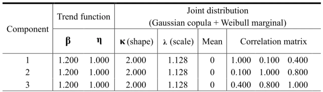
3.2.5.1 Hypothesis Test for Clayton Copula ... 47 3.2.5.2 Hypothesis Test for Gaussian Copula ... 48 3.2.6 Simulation Study ... 48 3.2.6.1 Parameter Setting ... 49 3.2.6.2 Parameter Estimation ... 52 3.2.6.3 Case Study ... 56 3.3 Conclusion ... 60 CHAPTER 4. INSPECTION-BASED OPTIMAL MAINTENANCE PLANNING .. 62 4.1 Developed Maintenance Policies ... 62 4.2 Optimization of Maintenance Policies ... 63 4.2.1 Optimization of MP I ... 64 4.2.2 Optimization of MP II ... 66 4.3 Case Study ... 70 4.3.1 Optimal Maintenance Policies ... 70 4.3.2 Comparison of Maintenance Planning Results with and without Considering Failure Dependency ... 72 4.4 Conclusion ... 73 CHAPTER 5. GENERAL CONCLUSIONS ... 75 APPENDIX 1. Generation of Latent Ages to Failure from Truncated Distribution Constructed via Gaussian Copula ... 77 APPENDIX 2. FDSA Algorithm Applied in MP II for Optimization ... 78 APPENDIX 3. Proof of Proposition 3 ... 79 APPENDIX 4. Proof of Equation 29 ... 82
APPENDIX 5. Procedure to Simulate the Failure Data of A K-component System Based on the Proposed CTP Model ... 84 REFERENCES ... 86 ABSTRACT ... 97 AUTOBIOGRAPHICAL STATEMENT ... 99
LIST OF TABLES
Table 1. Parameter setting in simulation Scenario I ... 33
Table 2. Parameter setting in simulation Scenario II ... 33
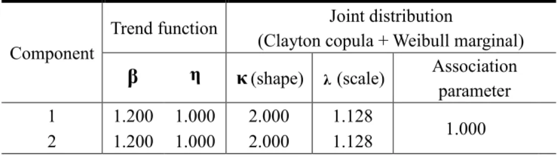
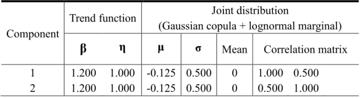
Table 3. Estimated parameters and the standard errors when using bivariate lognormal distribution ... 36 Table 4. Estimated parameters and the standard errors when using bivariate Weibull constructed via Gaussian copula ... 37 Table 5. Parameter setting in simulation Scenario I (Gaussian copula) ... 49 Table 6. Parameter setting in simulation Scenario I (Clayton copula) ... 50 Table 7. Parameter setting in simulation Scenario III (lognormal marginal) ... 51 Table 8. Parameter setting in simulation Scenario V ... 52
Table 9. Parameter estimates and standard errors (values in the bracket) when choosing the Clayton copula ... 58
Table 10. Parameter estimates and standard errors (values in the bracket) when choosing the Gaussian copula ... 58
Table 11. Maximum log-likelihood values for pair-wise dependency tests ... 59
Table 12. p-values for dependency test from Gaussian copula ... 59
Table 13. Cost parameter setting in the maintenance ... 70
Table 14. Optimal MP II results with four combinations of repair effectiveness levels ... 71
Table 15. Real and estimated parameters with and without considering failure dependency ... 72
LIST OF FIGURES
Fig. 1. Illustrations of the first (left), and the second (right) failures in a competing
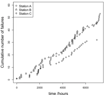
risks system ...11 Fig. 2.Illustration of the GDLA model using a two-component repairable system ... 29 Fig. 3. Simulation results with parameter setting in Table 1 ... 34 Fig. 4. Simulation results with parameter setting in Table 2 ... 34 Fig. 5. Failure data of two stations from an assembling cell ... 36 Fig. 6. System reliabilities after a repair vs. time and initial ages (I: the initial age of component 2 is zero; II: the initial age of component 1 is zero). ... 38 Fig. 7. Illustration of the multiple transformation procedure based on different trend functions for different failure types ... 40 Fig. 8. Simulation results for scenario 1 with Clayton copula ... 53 Fig. 9. Simulation results for scenario 1 with Gaussian copula. ... 53 Fig. 10. Simulation results for scenario 2 with independent failures... 54 Fig. 11. Simulation results for scenario 2 with high dependency ... 54 Fig. 12. Simulation results for scenario 3 with lognormal marginal ... 55 Fig. 13. Simulation results for scenario 4 with constant trend function ... 55 Fig. 14. Simulation results for scenario 4 with decreasing trend functions ... 56 Fig. 15. Simulation results for scenario 5 with 3 stations ... 56 Fig. 16. Failure data from stations A, B and C ... 57 Fig. 17. MP I (left) and MP II (right) for a two-component system ... 63 Fig. 18.Simulation-based optimization method with stochastic approximation ... 67
CHAPTER 1. INTRODUCTION 1.1 Background
Reliability analysis of multi-component repairable systems plays a critical role for system safety and cost reduction. A variety of multi-component systems are subject to competing risks (David and Moeschberger 1978, Meeker and Escobar 1998, Crowder 2010, Hong and Meeker 2014). Under competing risks, only the failure with the smallest latent failure time can be observed. Competing risks theory seeks to provide the statistical relations between all the latent failure times associated with different failure types that cannot be observed directly (Bedford and Alkali 2009). In competing risks systems, different risks can be dependent. For example, consider a vehicle’s transmission system in which transmission fluid is used to lubricate the moving parts. The wearing out of the transmission fluid can cause both the clutches and the gears to deteriorate significantly. And failure of either the clutch or the gear can cause the failure of the transmission system. Thus, the clutches and the gears suffer from dependent competing risks. In general, ignoring the failure dependency of multiple components can result in biased predictions of system reliability and non-optimality of the maintenance policy. In addition, in most cases, only the failed component (e.g., either the failed clutch or the failed gear) is repaired, and the repair can be general, including perfect replacement and minimal
repair, as well as the situations in between.
There are three prominent aspects which pose as major challenges of building a reliability model and developing maintenance planning for dependent competing risks systems with imperfect repair. First, when the system fails, the failure time data of the un-failed components are right-censored. In other words, only the failure time of the failed component is recorded, while the latent failure times of all the other components cannot be observed due to competing risks. Second, when considering the dependency of competing risks, one component’s failure and repair will influence other components’ lifetimes. The influence of an imperfect component repair is more complex than a perfect repair that restores the component as good as new. Third, when considering dependent competing risks and general repairs, complex optimization problems arise for new maintenance policies.
1.2 Literature Review
Traditional study on repairable systems mainly focuses on reliability modes for repairable systems with a single component under different repair actions. Kijima and Sumita (1986) and Kijima (1989) suggested two imperfect repair models by introducing the concept of virtual age of repairable systems. Lindqvist, Elvebakk, et al. (2003) proposed a Trend-renewal Process (TRP) to generalize the inhomogeneous and
modulated gamma process proposed by Berman (Berman 1981), which can deal with the imperfect repair conditions well. Other imperfect repair models for repairable systems with a single component include the modulated renewal process (Cox 1972), the modulated power law process (Lakey and Rigdon 1992), the arithmetic reduction of age and arithmetic reduction of intensity models (Doyen and Gaudoin 2004), the stochastic general repair model (Guo, Haitao, et al. 2007). A comprehensive review on statistical methods of repairable systems is provided by Lindqvist (2006).
For repairable systems under competing risks, most of the existing research assumes independency of component failure (Pham and Wang 2000, Langseth and Lindqvist 2006, Wang, Chu, et al. 2009, Yang and Chen 2009, Hong and Meeker 2010, Yang and Chen 2010, 2011, Yang, Hong, et al. 2012). Thus, the reliability analysis of the entire system subjected to competing risks can be simplified by analyzing each component independently. The existing reliability models that consider failure dependency assume that when a failure of one component occurs, it will result in a possible shock to the other components with a certain probability (Jhang and Sheu 2000, Scarf and Deara 2002, Satow and Osaki 2003, Zequeira and Bérenguer 2005a, Barros, Berenguer, et al. 2006). Li and Pham (2005) discussed a similar system with component failure dependency, and they assumed a binomial distribution of perfect and minimal repairs with certain
multiple components associated with failures caused by multiple sources. Shaked and Shanthikumar (1986) developed statistical models and investigated properties of repairable systems with dependent component failures. However, in their work, the parameters estimation approach was not given and the repair actions were not considered. In the past decades, maintenance study for multi-component system has attracted more and more attention. The main objective of maintenance is to retain or restore a system to perform its required functions satisfactorily. For simple system with a single component, there has been lots of maintenance models based on different assumptions (Lee and Rosenblatt 1989, Bunks, McCarthy, et al. 2000, Grall, Bérenguer, et al. 2002, Marseguerra, Zio, et al. 2002, Wang 2002, Aghezzaf, Jamali, et al. 2007, Peng, Feng, et al. 2011). The definition of multi-component maintenance is defined as: multi component maintenance models are concerned with optimal maintenance policies for a system consisting of several units of machines or many pieces of equipment, which may or may not depend on each other (Cho and Parlar 1991). If there is no dependency, then we can apply the single component maintenance policy on each component of the multi-component system separately. However, the dependency always is not negligible; for example, the down time of the system, which is shared among all components, will cause the economic dependency. When components form a system structurally so that the maintenance of failed component always involves maintenance of other components, it is
called structural dependency (Nowakowski and Werbińka 2009). In addition, Murthy introduced three types of stochastic dependency considering failure interaction (Murthy and Nguyen 1985a, b).
Generally, the maintenance can be divided into two main types, i.e., corrective maintenance and preventive maintenance (Nowakowski and Werbińka 2009). Corrective maintenance means the failed component or system will be repaired perfectly immediately after the failure. Due to the limited maintenance resource in reality, immediate repair is difficult to implement, which is the big disadvantage of corrective maintenance. Preventative maintenance is used to describe the maintenance before failure occurs (Valdez-Flores and Feldman 1989). In the literature, block replacement policy is the most well-known preventive maintenance policy (Barlow and Hunter 1960). In such a policy, the components are commonly replaced on periodical intervals or failures (Berg and Epstein 1976). There are various modifications of block replacement policy (Tango 1978, Nakagawa 1986). Scarf and Deara (2002) proposed various block replacement policies considering type I failure interaction as the stochastic dependency, i.e., either component’s failure can induce the other’s failure in a two-component system. The major drawback of block replacement policy is the waste of components or system replacement even if sometimes it is not necessary. Inspection-based maintenance is another commonly
al. 2000, Kallen and van Noortwijk 2005, Zequeira and Bérenguer 2005b, Wang 2009). Under the inspection maintenance, replacement can only be done after the detection of failures on inspections. Thus inspection maintenance policy can avoid the waste of unnecessary replacement in block replacement. Taghipour applied the periodic inspection maintenance for a multi-component system with non-competing risks (Taghipour and Banjevic 2011). Compared with non-competing risks system, the reliability modeling and maintenance planning is more complex as we cannot observe the full failure events due to competing risks. Few studies can be found on the maintenance planning of multi-component systems considering dependent competing risks.
1.3 Research Objectives
In this research, we focus on the repairable multi-component systems under competing risks. The dependency of different component failures is not clear thus we do not make any prior assumption whether different components are independent or not. The key objectives of this research are listed as follows: 1. To establish parametric reliability models to investigate the statistical dependency of multi-component systems under competing risks with imperfect repair. 2. To study optimal inspection-based maintenance planning for multi-component system under dependent competing risks.
1.4 Dissertation Organization
The dissertation consists of three main chapters, preceded by an introduction in the present chapter and followed by a conclusion. CHAPTER 2 presents a statistical model for multi-component repairable systems under dependent competing risks with partially perfect repair assumptions. CHAPTER 3 studies two statistical models considering generally imperfect repair and dependent competing risks for multi-component repairable systems. CHAPTER 4 presents two inspection-based maintenance policies based on the proposed reliability model.
CHAPTER 2. RELIABILITY ANALYSIS OF MULTI-COMPONENT SYSTEMS WITH DEPENDENT COMPETING RISKS UNDER PARTIALLY PERFECT
REPAIR 2.1 Data Notation
We consider a competing-risk system consisting of multiple (say K) components.
The time scale is the time since installation. Upon each failure, only the failed component is repaired as good as new and the other components are untouched, which is called partially perfect repair. In general, the partially perfect repair is achieved by replacing the
failed component with a new one. The successive failure events are recorded by T T1, 2,...,
until a predetermined ending time . In addition, each event is labeled with a failure
type i {0,1,..., }K ; where i 0 indicates there is no failure observed. We use pair
( ,Ti i) to represent failure information. An equivalent representation of the failure
process is in terms of the marked point process {N t tk( ); 0,k 1,..., }K ; where k
denotes failure type and N tk( ) denotes the cumulative number of failures for
component k until time t. We use
1
( ) K k( )
k
N t N t
to denote the total number offailures regardless of failure type until time t. We assume that two failures cannot occur
simultaneously, which is a common assumption for repairable systems in the literature. In addition, we assume the repair action is immediate and the repair time is ignored.
2.2 Statistical Modeling for Multiple Dependent Competing Risks under Partially Perfect Repair
In the classical latent failure times model (Prentice, Kalbfleisch, et al. 1978), a single-component system has multiple competing failure types, each of which can cause the system’s failure. Each failure type has a failure time, but only the minimum can be observed due to competing risks. Because of unobservable nature, the failure times are also called conceptual or latent failure times, which are generally assumed to follow a joint distribution to capture the dependency of competing risks.
Consider a system that consists of K new components starting to work at time 0.
Because the components are under competing risks, the system fails if any component fails, while the failure time of all the other components cannot be observed.
Let r tk( ) be the most recent failure time of component k before time t. The
running time of component k at time t since its last replacement, which is defined as
age and is denoted as a tk( ), can be calculated as a tk( ) t r tk( ). Note that both r tk( )
and a tk( ) are defined as left-continuous functions. Thus, k( ) lim ( )k
x t
r t r x
if a failure
occurs at time t , and r tk( )0 if no failure occurred by time t . Similarly,
( ) lim ( ) k k x t a t a x .
We use Zk i, to denote the latent age of component k to the system’s ith failure.
th
i
failure for all components. Due to competing risks, only the minimum of latent agesto failure can be observed. Similar to the classical latent failure times model, we also use
a joint distribution F to model Zi like the classical latent failure times model if the
system is either new or perfectly repaired. The dependency of component failures is
captured by the joint distribution F. The next failure time of the system on or after time t is determined as the minimum value of { k( ) , ( ) 1 k N t r t Z
, k 1, 2,...,K } (N t( ) denotes its left limit at time t) under
the condition that
, ( ) 1 k( )
k N t
Z a t , k 1, 2,...,K. Fig. 1 illustrates the first two failures in
a competing risks system. Let vector z1[z1,1,...,zK,1]T be the realization of the latent
ages to the first system’s failure Z1.The first failure is determined by the minimal value
of zk,1; k 1,...,K . Suppose the first failure is due to component l and occurs at time
1
t (Fig. 1 left). Under partially perfect repair assumptions, only component l is
replaced, and the most recent failure times are updated as r tl( )t1, and r tj( )0, jl,
1,...,
j K . The second failure can be calculated as the minimum value of
,2 1 , 2 {zl t z, j ;jl j, 1, ...,K} (Fig. 1 right), where 2 [ 1,2,..., ,2] T K z z z is the realization of the latent ages to the second system’s failure.
1,1 z ,1 i z 1 t ,1 K z 1 1( ) 0 r t 1 ( ) 0 l r t 1 ( ) 0 K r t component 1 component l component K 1,2 z ,2 l z 2 t ,2 K z 1( ) 02 r t 2 1 ( ) l r t t 2 ( ) 0 K r t component K component l component 1 0 Fig. 1. Illustrations of the first (left), and the second (right) failures in a competing risks system , 1 k i
Z , the latent age of component k to ( 1)
th
i system’s failure, should be larger
than the age of component k immediately after time ti, i.e., Zk i, 1 a tk
i (a tk
idenotes its right limit at time ti), k {1,..., };K i1, 2,.... As a result, the random
vector 1 [ 1, 1, ..., , 1]T
i Z i ZK i
Z is following a truncated distribution of F conditional on
the vector of
[
a t
1
i, ,
a t
K
i]
T.2.3 Parametric Forms
The joint distribution of the random vector Zi describes the statistical failure
mechanism of multiple components, and thus captures their statistical failure dependency. In this section, parametric models are proposed to characterize the joint distribution of
i
Z .
As Weibull and lognormal distributions are commonly used as failure time distributions for single-component systems (Barlow and Proschan 1975, Jordan 1978, Prabhakar Murthy, Bulmer, et al. 2004, Pascual, Meeker, et al. 2006), they are separately
selected as the marginals of the joint distribution F to illustrate the proposed method in
this research. However, other proper univariate distributions can also be applied.
2.3.1 Parametric Forms for Multivariate Lognormal Distribution
When the joint distribution of random vector Zi is multivariate lognormal, the joint probability density function (pdf) is calculated as:
1
1/2 /2 1 1( ; , ) exp log( ) log( )
2 (2 ) T i K i i f z μ Σ z μ Σ z μ Σ . (1)
The model parameters θ include μ and Σ. μRK, and ΣRK K are the mean
vector, and covariance matrix of the multivariate lognormal, respectively.
2.3.2 Parametric Forms for Multivariate Weibull Distribution via Archimedean Copula Function The cumulative distribution function (cdf) of the Weibull marginal Fk is: , , , ( ; ) 1 exp ; 0 k k i k k i k k i k z F z z θ (2)
where k(0, ) and k(0, ) are called shape and scale parameter, respectively.
[ , ] k k T k θ is the parameter vector of the marginal distribution Fk. We can construct the joint distribution from marginal Weibull by using Archimedean copula functions.
The Archimedean family of copulas are frequently used for the construction of multivariate distributions due to their simple forms (Nelsen 2006)
C u( ,1 ,uK) 1( )u1 1(uK)
(3)
where is the generator of the Archimedean copula. Different generators will generate
different Archimedean copulas. For example, ( )t (1 t)1/
, and ( )t exp(t1/)
are generators for Clayton, and Gumbel-Hougaard copulas, respectively.
In this research, the Clayton copula is selected as an example to illustrate the application of the Archimedean copula family in the proposed reliability model. Clayton
copula contains one association parameter that relates to the dependency
measurement Kendall’s tau K endall (Lindskog, McNeil, et al. 2003), by the relation
( 2)
Kendall
(Nelsen 2006).
When the Clayton copula is selected to construct the joint distribution, the
dependency of the failure types is captured by the association parameter . The range of
the association parameter is [ 1, 0)(0, ) . The limiting case when
0represents the independent situation. In this research, we define the Clayton copula as follows: 1/ 1 1 1 max 1, 0 ; 0 ( , , ) ; 0 K k k Clayton K K k k u K C u u u
(4)can be obtained by substituting uk 1 exp
zk,i/ k
k
into (4), where 1 { ,..., K, } θ θ θ .2.3.3 Parametric Forms for Multivariate Weibull Distribution via the Gaussian Copula Function
The Gaussian copula is a special copula taking advantage of the pdf of the multivariate normal distribution (Cherubini, Luciano, et al. 2004). Specifically, a Gaussian copula has the form CGauss(u1,, ,uK) [ 1( ),u1 , 1(uK)] (5) where 1 is the inverse of the cdf of the standard normal distribution, and is the cdf of a multivariate normal distribution with zero mean vector, and its covariance matrix equals its correlation matrix. The Gaussian copula density function is given as (Song 2000) 1 1 1 1 1 1 1/2 1 1 ( ) ( ) 1 1 ( , , ) exp ( ) 2 ( ) ( ) T Gauss K K K u u c u u u u Σ I Σ (6)
where Σ is the correlation matrix, and I is the identity matrix.
When applying a Gaussian copula to construct the joint Weibull distribution, the
1, , 1, , 1, ,
( ; ) ( , , )
i K i
i z z Gauss i K i i K i
S z θ
f x x dx dx (7)where fGauss( ) denotes the pdf of the joint Weibull distribution obtained by the chain
rule, i.e., 1 1, ,i 1 1, , 1 1 1, 1 , ( , , ) ( , ) ( ; ) ( ; ) K Gauss K Gauss i K K i K i Gauss K i K K i K C du du f z z u u dz dz c u u f z f z θ θ (8) and fk( ); k1,...,K denotes the pdf of the marginal for Zk i, .
In the multivariate Weibull distribution constructed via the Gaussian copula, the
model parameter θ{ ,...,θ1 θK, }Σ .
2.4 Parameters Estimation Based on Maximum Likelihood Method
A maximum likelihood (ML) method is developed to estimate model parameters. To
implement the ML approach, we first calculate the likelihood function. Suppose the ith
failure is due to component k, and occurs at time ti. The latent age to ith system failure
of component k is equal to a tk( )i , while the latent ages of all other components should
be larger than a tj( );i jk j, 1, ...,K . Thus, the unconditional probability to observe
failure i is calculated as
1, 1 , , 1, , , , , , ( ) , ( ), , ( ) , Pr( ( ), ( ); , 1,..., ) , i k i k i i Ki K i i k i k i j K i j i k i a t a t i a t z z z S z z z Z a t Z a t j k j K . (9)Note that (10) gives the probability at a given time t for a continuous random
variable. Although technically
Pr(
X
t
) 0
for a continuous random variable X withpdf f t( ) , Pr(X t) can be interpreted as Pr(tX t dt) f t dt( ) , which is
proportional to f t( ). We ignore dt only for notational convenience in the calculation
of the likelihood function for all continuous random variables in the rest of the dissertation.
Equation (9) only accounts for the probability of an observed failure at time ti
regardless of previous failure data. The conditional probability of observing failure i
given all the previous i1 failures is solely determined by the ages of all components
after the repair action of the (i1)th failure. Specifically, the likelihood of failure i,
1, 2, , ( ) i N , conditioned on all the previous i1 failures, can be calculated as
1, 1 , , , ( ) ( 1, ) ( , , , , ) 1 , 1 1 ( ) , , , ( , ) i i k i k i K i K i k i a t a i t a t i i z z z K i K i S S z z a t a t z (10) where S( ) is the joint survival function of the latent ages to failures.For example, consider the first two failures illustrated in Fig. 1. After the repair
action of the first failure at time t1, the age of the failed component l is updated to
1
( ) 0
l
a t , while the ages of all the other components are given as
1 1
( )
j
, 1,...,
jl j K. As the second failure is due to component one, and occurs at time t2,
the likelihood of the second failure conditioned on the first failure can be calculated as
1,2 1 2 , 2 2 , 2 ,2 1 Pr(Z a t( ),Zj a tj( ); j1, j1, ...,K Z| l 0,Zk t k; l k, 1, ...,K) , where 2 2 1 ( ) l a t t t , and a tj( )2 t2;j l j, 1, ...,K .
As there is no failure observed from tN( ) to the predetermined ending time , the
likelihood N( ) 1 can be calculated as
1, ( ) 1 1 , ( ) 1 ( ) 1 1 ( ) ( ) 1 1 ( ) ( ) Pr{ [ ( )],..., [ ( )]} ( ),..., ( ) ( ),..., ( ) ( ),..., ( ) N K N K N N K N K N K N Z r Z r S a t a t S a t a t S a t a t . (11)Combining the results in (10) and (11), the following Proposition 1 can be used to calculate the likelihood function based on the observed failure data.
Proposition 1. Given the observed failure data, the likelihood function can be calculated by ( ) 1 1 ( ) N i i
θ (12)where i can be calculated based on (10), and (11) for i1,2,, ( )N
, and( ) 1
The estimated model parameters ˆθ are obtained by maximizing ( )θ . Based on the
ML theory (Svensson 1990, Casella and Berger 2001), the estimated parameters ˆθ are
asymptotically normally distributed under the large sample assumption.
2.5 Hypothesis Testing for Dependency
Based on the proposed reliability model for the competing risks systems, statistical hypothesis testing procedures are developed in this section to determine the component failure dependencies. In Section 2.5.1, a dependency test based on the multivariate lognormal distribution is proposed. Then in Section 2.5.2, a dependency test for the multivariate Weibull distribution derived by the Archimedean copula and the Gaussian copula are discussed, respectively.
2.5.1 A Dependency Test for the Multivariate Lognormal Distribution
In the multivariate lognormal distribution, the dependency information is captured by the correlation matrix Λ, which can be calculated based on covariance matrix Σ: , , , , ; , 1, , i j i j i i j j i j K Σ Λ Σ Σ (13)
where Λi j, , and Σi j, are the elements of the
th
i
row, and the jth column in Λ, and Σ,developed to determine the statistical dependency among latent ages to failures of components. H0: component failures
i j
,
are statistically independent. 1 H : component failuresi j
,
are statistically dependent. (14)When the asymptotic result is applied, we use a normal approximation to construct
the test statistics. The test statistics Wi j, are used to test the dependency between
component failures i and j, which equals the estimate of correlation Λˆi j, divided by
its estimated standard error var(Λˆi j, ), i.e.,
Wi j, Λˆi j, / var(Λˆi j, ). (15)
In hypothesis testing (14), H0 is rejected if Wi j, Z/ 2, or Wi j, Z1/ 2, where is
the test significance level, and Z/2 is the upper quantile of the standard normal
distribution. Based on hypothesis testing (14), pairwise statistical dependencies between different component failures can be tested.
2.5.2 A Dependency Test for the Multivariate Weibull Distribution
In this section, a statistical dependency test for joint distribution constructed via the
Archimedean copula is first discussed. The Archimedean copula can capture the overall
developed the following hypothesis testing procedure to test the overall failure dependency, i.e., to see whether Kendall’s tau is equal to zero. H0: all failure types are statistically independent. 1 H : not all failure types are statistically independent. (16)
Here, the asymptotic test statistic Woverall is constructed using the estimate of
Kendall’s tau ˆKendall divided by its estimated standard error var(ˆKendall) . H0 is
rejected if Woverall Z/2 or Woverall Z1/2. As Kendall’s tau is a function of the
association parameter , the variance of the estimate of Kendall’s tau can be calculated by using the delta method.
ˆ 2 2 ˆ ˆ ˆ ˆ var( ) ( ) var( )( ) ˆ ˆ ˆ (ˆ/ ( ˆ 2) 1 / ˆ var( ) ( 2)) T Kendall Kendall Kendall d d d d (17)where var( )ˆ denotes the asymptotic variance of
ˆ. Based on (17), the asymptotic teststatistic of the overall dependency is given as
2 2
2 ˆ ˆ ˆ ˆ ˆ ˆ var( ) ( / ( 2) 1/ ( 2 )) Kendall overall W . (18)For the multivariate Weibull distribution constructed via the Gaussian copula, the correlation matrix determines the pairwise dependencies of latent ages to component
failures. Thus, the test procedure is the same as that discussed for the multivariate lognormal distribution.
The test statistics for Multivariate Weibull via the Gaussian copula has the same form as (15). Thus, hypothesis testing (14) can be used here to test the pairwise statistical dependencies among different failure types.
2.6 Conclusion
In this Chapter, a general statistical reliability model is proposed for repairable multi-component systems considering statistical dependent competing risks under a partially perfect repair assumption. For the reliability analysis of repairable multi-component systems, most of the research in the literature assumes component failure statistical independency. The failure mechanism (marginal distribution) of each component can thus be estimated individually based on its failure data.
In the developed model, copula functions are used to model the joint distribution of component failure times. Specifically, two types of copulas, i.e., the Archimedean copula, and the Gaussian copula, are applied to study the overall dependency, and pairwise dependencies among different components, respectively. Although the copula function method is also applied in the literature to study non-repairable systems, or systems under perfect repair action (replace the whole system when a failure happens), the problem
studied in this paper is much more complex than those in the literature. When the whole system is replaced after a failure, the system will have the same failure mechanism as the original one. In contrast, when only the failed component is replaced, replacement of failed component affects the failure mechanism of the other components when considering failure dependency. Thus, the methods in the literature cannot be directly applied.
Under competing risks assumptions, only the failed component is recorded as the latent ages to failures of other components cannot be observed. After a repair action under the partially perfect repair assumption, the failure mechanism of the new system and components will be changed. Thus, for a single repairable system in which the failure data can only be collected from a single realization, model parameters estimation is challenging. To tackle this problem, an ML method is developed in this research, and the ML function is calculated based on conditional probability.
The partially perfect repair action is useful for many complex multi-component engineering systems when only the failed component is repaired, and the repair action is a replacement due to high labor cost.
Hypothesis testing is developed to test the statistical dependency of component failures. The obtained statistical failure dependency provides more accurate information for reliability predictions, which can be used for system maintenance.
The proposed methodology in this Chapter has been published in a journal article (Yang, Zhang, et al. 2013).
CHAPTER 3. RELIABILITY ANALYSIS OF MULTI-COMPONENT SYSTEMS REPAIRABLE SYSTEMS WITH DEPENDENT COMPETING RISKS UNDER
IMPERFECT REPAIR
In previous Chapter, statistical model for repairable multi-component systems with partially perfect repair is proposed. However, in most cases, the repair conditions are unknown. Thus, the partially perfect repair assumption may not always hold. Thus, in this Chapter, we extend the model proposed in previous Chapter from partially perfect repair conditions to generally imperfect repair conditions. Specifically, two models are proposed, i.e., the generalized dependent latent age model and the copula-based trend-renewal process model.
3.1 Generalized Dependent Latent Age Model
The generalized dependent latent age model (GDLA) model generalizes partially perfect repair model proposed in CHAPTER 2 by extending Kijima’s virtual age models (Kijima and Sumita 1986, Kijima 1989) from repairable single-component systems to multi-component systems.
In this research, we are interested in repairable K -component systems under
competing risks. The failures of the same component are regarded as one type of failures. After each failure, the failed component is repaired and other components are untouched. The repair conditions for the failed components are imperfect, including the two extreme
cases, i.e., minimal repair and perfect repair. The partially perfect repair condition discussed in CHAPTER 2 is a special case of the imperfect repair conditions.
To deal with generally imperfect repairs of multi-component systems, we first extend Kijima’s virtual age models from single-component systems to multi-component systems and then combine it with the partially perfect repair model to develop the GDLA model.
3.1.1 Extended Virtual Ages for Multi-component Systems
Two virtual age models are developed for repairable single-component systems in
(Kijima and Sumita 1986, Kijima 1989). Let t t1, ,...2 , denote the failure time series
(t0 0), and let xi ti ti1;i1, 2,..., denote the inter-arrival times of failures. The
virtual age is used to describe the system state. Specifically, after the ith repair, the
virtual age vi in Kijima model I and II is defined as vi vi1 q xi and
1
( )
i i i
v q v x respectively, where q[0,1] is the repair effectiveness factor. q0
and q1 correspond to the two extreme repair cases, i.e., perfect repair and minimal
repair respectively; and
q
0,1
corresponds to the imperfect repairs.For the repairable K-component system, we extend the Kijima model II to describe
the state of multiple components. Let ;t ii 1, 2,..., denote the observed failure time of the
th
i failure (t0 0), and let r t ll( ); {1,..., }K be the most recent failure time of
( ) 0; if 0 ( ) ( ); if ( ) and 0 ( ) ( ( )) ( ( )); if ( ) l l l l l l l l l l v t t v t q v t t r t t v t v r t t r t t r t (19)
where v tl( ) is right-continuous and v tl( ) denotes its left limit at time t, and ql
represents the repair effectiveness factor of component l. In (19), t r tl( ) indicates
that there is a failure from component l which occurs at time t. It is worthwhile to note
that the age a tl( ) defined in CHAPTER 2 is left-continuous, compared with the
right-continuous virtual age v tl( ).
As the repair effectiveness factors are not necessary to be the same for different
components, we use a constant vector [ 1, ..., ]T
K
q q
q to denote the repair effectiveness
factor for the entire system. As ql[0,1], the extended virtual age model for
multi-component systems can deal with generally imperfect repairs, including the perfect replacement and minimal repairs. Ideally, when the repairs are either perfect or minimal, the repair effectiveness factors can be directly recorded. However, under many situations the repair effectiveness is difficult to be quantified. Thus, it is more reasonable to assume 1 [q , ...,qK]T q is an unknown vector which also needs to be estimated from the failure
data. The estimated repair effectiveness factors can be further used in the maintenance planning.
3.1.2 Model Building
Based on partially perfect repair reliability model and the extended virtual ages, we propose the GDLA model to deal with both generally imperfect repairs and dependent competing risks.
We use the term initial ages to represent the virtual ages of all components after the
system’s ith repair, which are denoted as [ 1
i , ,
i ]T K v t v t . For i0 ,
1 [v ti ,,vK ti ]T [0,...,0]T; and fori
1,2,...
, [ 1
i , ,
i ] T K v t v t can be calculated as a function of repair effectiveness factor q [q1, ...,qK]T according to (19).The GDLA model assumes that once a component’s virtual age reaches a corresponding threshold, the component fails, which causes the entire system’s failure. Thus, the random threshold corresponds to the latent age to failure concept which has
been used in CHAPTER 2. We still use Zk i, to denote the latent age of component k to
the system’s ith failure which is defined in the partially perfect repair reliability model,
and the random vector Zi [Z1,i,...,ZK i,]T represents the latent ages to the system’s
i
thfailure for all components. Due to competing risks, only the minimum of latent ages to
failure can be observed. In the GDLA model, we also use a joint distribution F to
model Zi like the partially perfect repair model. The dependency of component failures
failure must be larger than its initial age, i.e., Zl, 1i v tl
i , l {1,..., }K . In otherwords, the latent ages to the (i1)th system’s failure Zi1 are following a truncated
distribution conditional on the initial ages [v t1
i ,,vK
ti ]T . When the failedcomponent is repaired as good as new, the GDLA model degenerates to the reliability model proposed in CHAPTER 2 under partially perfect repair conditions.
An example that illustrates the extended virtual ages and the proposed GDLA model
is given in Fig. 1, where paired (ti,i) denotes the failure time ti and the failed
component i for the ith failure. The first observed failure comes from component 1 at
1
t , since the age of component 1 reaches its latent age to failure Z1,1 before the age of
component 2 reaches Z2,1. The second observed failure comes from component 2 at t2,
since Z2,2 is reached ahead of Z1,2. The next failure still comes from component 2 as
2,3
2 ( ,2)t 1 ( ,1)t 0 1,1 Z 2,1 Z 1,2 Z 2,2 Z 3 ( ,2)t 2,3 Z 1,3 Z System virtual age of component 1 virtual age of component 2 Fig. 2.Illustration of the GDLA model using a two-component repairable system
We construct the joint distribution in the way as the partially perfect repair model. More specifically, the Weibull and lognormal distributions are separately selected as the
marginals of the joint distribution F and copula functions are used to construct the joint
distribution to illustrate the proposed method in this research.
When the marginal is chosen as lognormal, the multivariate lognormal distribution is
generally used as the joint distribution F . The proposed model parameters are denoted
by θ{q,μ Σ, }, where μRK is the mean vector and Σ is the K K covariance
matrix, respectively. The cdf of the joint Weibull distribution constructed via Gaussian copula is: FG
z1,i, ,zK i, |
Φ
Φ (1 u1,i), , Φ (1 uK i,)
θ Σ (20) whereu
1 exp
(
z
/ )
kl
multivariate normal distribution with a zero mean vector requiring its covariance matrix
be equal to its correlation matrix; and Φ1 is the inverse cdf of the standard normal
distribution. The parameters for the reliability model with the Gaussian copula function
and marginal Weibull are denoted by θ{q,λ κ Σ, , }, where λ
1,,K
T and
1, ,
T K κ are the scale and shape parameters of Weibull distribution respectively; and Σ is the correlation matrix in ΦΣ.3.1.3 Parameter Estimation for the GDLA Model
We estimate the parameters in the GDLA model using the maximum likelihood
estimation (MLE) method. The overall likelihood function for n observed failure events equals:
1 n i i
θ (21)where i denotes the likelihood function of the ith failure conditional on the initial
ages of components after the (i1)th failure and the corresponding repair. Proposition 2
is developed to calculate the likelihood function i.
Proposition 2. Suppose the ith failure comes from component j ; the initial ages
1 1 , , 1
[v ti vK ti ]T can be obtained by (19) as a function of unknown repair
effectiveness factor q [q1, ...,qK]T . Then the likelihood function of the ith failure
1 , 1, , , , , 1, 1 , 1, 1 1 , 1 1, 1 , 1, 1 1 1 , 1 1, , , , , , , Pr , , , , , , Pr , , , , Pr , , , , , , i i j i j i K i i i i i K i K i i i K i K i i i i K i K i i i i K i K i i K i z v t z v t z v j i j j i j j i j j i Z v t Z v t Z v t Z v t Z v t Z v t Z v t Z v t Z v t Z v t Z v t S z z z
1 1 , , 1 , , 1
K ti i j i K i S v t v t v t (22) where S( ) is the joint survival function of the latent ages to failure. Presenting a two-component system as an example, the first failure observed at time5 came from component 2, and the second failure observed at time 20 came from component 1. Then, the likelihood for the first failure is calculated as
1Pr Z1,15,Z2,15Z1,10,Z2,10
. For the repaired system, the latent ages to the
first system’s failure for component 1 was exactly 20 given its initial age 5, while that for
component 2 was larger than (15q25) given its initial age q25. Thus, the likelihood
for the second observed failure 2 Pr
Z1,2 20,Z2,2 ( 51 q25) Z1,2 5,Z2,2 q25
.The parameters in the proposed model can be estimated by maximizing the overall likelihood function obtained in (21). Under a large sample assumption, the maximum likelihood estimates are asymptotically normally distributed, and the covariance matrix can be calculated by the inverse of the observed Fisher information matrix (Casella and Berger 2001). Due to the complexity of the likelihood function (21), the analytical
numerical optimization method, i.e., the simulated annealing algorithm to maximize (21) (Bélisle 1992).
3.1.4 System Reliability Prediction
The reliability of the system after the ith repair can be predicted using the proposed
reliability model. Let Tmin denote the inter-arrival time between the ith repair and the
(i1)th failure, and let
min T
F denote the cdf of the random variable Tmin. The system
reliability at time t since the ith repair is calculated as:
1 1 1 , , | , , , , K K i i i i K i i S v t t v t t R t v t v t S v t v t . (23)where [v t1
i ,,vK
ti ]T are the initial ages and S( ) is the joint survival function oflatent ages to failure. When the joint distribution of latent ages is selected as multivariate
lognormal, the joint survival function S( ) is calculated by integrating its pdf.
3.1.5 Simulation Study
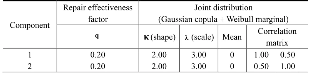
To verify the proposed reliability model and parameter estimation method, we conduct a simulation study for a two-component system. The failure data are simulated according to the GDLA model with joint distribution constructed with Gaussian copula and Weibull marginal. We consider failure dependency with different repair effectiveness factors in scenario I and II, whose parameters are listed in Table 1 and Table 2, respectively.
Table 1. Parameter setting in simulation Scenario I Component Repair effectiveness factor Joint distribution (Gaussian copula + Weibull marginal)
q κ(shape) λ (scale) Mean Correlation
matrix 1 0.20 2.00 3.00 0 1.00 0.50 2 0.20 2.00 3.00 0 0.50 1.00 Table 2. Parameter setting in simulation Scenario II Component Repair effectiveness factor Joint distribution (Gaussian copula + Weibull marginal)
q κ(shape) λ (scale) Mean Correlation
matrix
1 0.20 2.00 3.00 0 1.00 0.50
2 0.60 2.00 3.00 0 0.50 1.00
In each simulation scenario, we estimate the parameters with failure events n=100,
200, 500 and 1000 respectively. For each n, we conduct the simulations with 1000
replicates to obtain the coverage probabilities for the 95% confidence intervals and
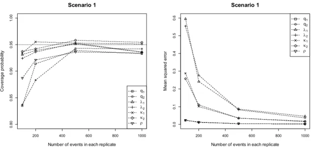
mean squared errors (MSE) for the parameter estimates. The simulation results of two scenarios are shown in Fig. 3 and Fig. 4, respectively.
Fig. 3. Simulation results with parameter setting in Table 1
Fig. 4. Simulation results with parameter setting in Table 2
In Fig. 3 and Fig. 4, it can be seen the coverage probabilities for the estimated
confidence intervals are approaching 95% and the MSEs are approaching zero as the number of failure/maintenance events increases, which validates the parameter estimation 200 400 600 800 1000 0. 8 0 0. 85 0 .90 0. 9 5 1. 0 0 Scenario 1
Number of events in each replicate
C o v e ra g e p ro b a b ili ty q1 q2 1 2 1 2 200 400 600 800 1000 0. 0 0. 1 0. 2 0 .3 0. 4 0 .5 0. 6 Scenario 1
Number of events in each replicate
M e an s q u a re d e rr o r q1 q2 1 2 1 2 200 400 600 800 1000 0 .8 0 0 .8 5 0 .9 0 0 .95 1. 0 0 Scenario 2
Number of events in each replicate
C o v e ra g e p ro b a b ilit y q1 q2 1 2 1 2 200 400 600 800 1000 0. 0 0 .2 0 .4 0 .6 0 .8 1 .0 1 .2 Scenario 2
Number of events in each replicate
Me a n s q u a re d e rr o r q1 q2 1 2 1 2