On Benchmarking Quantum Heuristics

On Benchmarking Quantum Heuristics

Zhihui Wang

IEEE Quantum Conference

Quantum AI Lab, NASA Ames Center

Universities Space Research Association

[email protected]

May 02 2019

Benchmarking quantum algorithms

• Quantum speedup:

• Any possible classical algorithms — Proven speedup, Shor, Grover

• State-of-art classical algorithms

• A general-purpose classical algorithm — E.g., SA, QMC

• A different type of algorithms: quantum heuristics

• Quantum annealing (QA)

• Variational quantum eigen solver (VQE)

• Quantum approximate optimization algorithm (QAOA)

Purpose:

Approximate optimization

Exact optimization

Sampling: specific distribution, fair sampling

Universal QC

No guaranteed speedup as a general algorithm

Universality proven through demonstrating ability

to generate universal basis sets.

suitable for NISQ device

[Rønnow, Wang, Job et. al., Defining and detecting quantum speedup, Science 2014]

Benchmarking quantum heuristics

Aspects

• Purpose:

— Approximate optimization

— Exact optimization

— Sampling: specific distribution, fair sampling

— Universal QC

• Metrics:

— approximation ratio

— prob-to-exact-solution,

— fairness, distance between distributions

— quantum complexity

• Additional Metrics for NISQ

— Circuit depth

All-to-all connectivity of physical qubits

Easier to scale connectivity (2D grid, Google bristlecone, Rigetti, IBM)

Logical quantum circuit to physical circuit: Circuit Compilation (gate scheduling)

Choice of basis gate sets

— Robustness

Variational nature will tolerate certain errors.

More actively sought fault-tolerance?

— Classical parameter setting

Analytical methods: deterministic parameters

How to update parameter values (gradient based, statistical optimization)

Quantum control landscape: local minima; barren plateau

— Benchmarking problem set

Typical vs worst-case

Small and hard

Illustrating using QAOA for graph coloring

• — Choice of Phase-Separator and Mixer

Use cost function (standard)

Specially designed: 1D chain with parity-dependent parameters (universal QC)

• — Choice of initial states

• — Measurement: What can we infer from the expected value / average performance?

— Circuit depth

All-to-all connectivity of physical qubits

Easier to scale connectivity (2D grid, Google bristlecone, Rigetti, IBM)

Logical quantum circuit to physical circuit: Circuit Compilation (gate scheduling)

Choice of basis gate sets

— Robustness

Variational nature will tolerate certain errors.

More actively sought fault-tolerance?

— Classical parameter setting

Analytical methods: deterministic parameters

Variational:

How to update parameter values (gradient based, statistical optimization)

Quantum control landscape: local minima; barren plateau

— Benchmarking problem set

Typical vs worst-case

One leading Candidate of quantum heuristics:

Q

uantum

A

pproximate

O

ptimization

A

lgorithms (QAOA) —>

Q

uantum

A

lternating

O

perator

A

nsatz

[Farhi, Goldstone, and Gutmann,

arXiv:1411.4028]

•

One-line summary of the algorithm

time

Cost

Mix

Choice of Mixer: QAOA for constrained optimization

•

How are constrained problems approached?

Encode the constraints as

penalty

in the cost function

. — Lagrange multipliers

Commonly practiced in quantum annealing.

Alternative

: Use a mixer/driver that contains the quantum evolution in the subspace

that satisfies the constraints.

Original motivation: Alleviate embedding burden

Another Advantage: Smaller search space!

We extend this idea to QAOA, formulate such mixers for a number of problems

and

study the performance of such alternate mixers

[Hen & Spedalieri, 2016]

Concept: [Hadfield, Wang, O'Gorman, Rieffel, Venturelli, Biswas, arXiv 1709.03489]; Performance & Circuit: [Wang, Rubin, Dominy, Rieffel, arXiv:1904.09314]

QAOA for graph coloring problem

•

Goal: Assign colors to vertices to maximize properly-colored edges (connecting two

vertices of different color)

Encoding

:

Binary: whether vertex v is assigned color-c

Constraints:

Each vertex should have exactly one color:

1

0

0

✓

✓

✓ ✓

Constraints:

Each vertex should have exactly one color:

Implemented as penalty in cost

:

Or

Stay in the feasible subspace

:

XY-model

Advantage:

Smaller search space: evolution contained in feasible subspace

Closer to hardware:

XY interaction (or iswap-gate) can naturally happen on certain

solid-state QC candidate systems

1

0

0

1

0

0

QAOA for graph coloring problem

8

decimal

one-hot Apply IXX decimal

0

000

011

3

1

001

010

2

2

010

001

1

3

011

000

0

4

100

111

7

5

101

110

6

6

110

110

5

7

111

100

4

Table I. Demonstration of deriving the partition corresponding to operator

IXX

on the binary encoding, Eq. (

25

)

.

model that increases the dimensions of the graph, such

as in the case where one-hot-encoding is used, simulating

the interaction term removes the necessity of encoding

techniques such as minor embedding or classical logical

encoding [

32

,

33

].

V.

SIMULATION RESULTS

In this section, we present the results of numerical

simulations of QAOA applied to the max-



-Colorable-Subgraph problem. We first compare the performance

of the

XY

mixer to that of the

X

mixer with penalty.

We then more deeply explore the behavior of

XY

mixers,

looking at general features of their performance on small

hard-to-color graphs, and comparing complete-graph

XY

mixers against ring

XY

mixers.

To acquire a good set of QAOA parameters,

stochas-tic optimizer is needed, in Appendix.

B

we show rugged

landscape with local optima in the parameter space that

would cause problem for deterministic optimizing

meth-ods like gradient descend. We instead use bsin-hopping

with BFGS to obtain (sub)optimal parameters.

A.

The death of

X

-mixer

We use a simple example, 2-coloring and 3-coloring of

a triangle to demonstrate the performance comparison of

XY

and

X

mixers.

Note that the penalty weight

↵

in general a

↵

ects the

performance of the algorithm. In Fig.

2

we show that

for 2-coloring the approximation ratio optimized over the

parameter set (

,

) for each penalty weight

↵

. The best

approximation ratio,

r

, takes value 0

.

75 while with

XY

driver QAOA

_p

₌₁

gets

r

= 1.

In Fig.

2, while the penalty strength has an e

↵

ect on

the behavior of level 1 QAOA, there appears to be no

clear intuition for choosing a good value. In particular,

the minimum penalty that guarantees the optimal state

being the optimal state in the feasible subspace,

indi-cated by the red arrows on the plots, does not stand out,

nor does the penalty value that guarantees separation

between energies feasible and infeasible states, indicated

by the the blue arrows. This supports our argument in

Sec. sec:penalty that the role of energy gap plays no clear

role in QAOA.

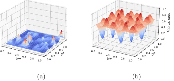
For 3-coloring, in Fig.

3

we plot how the approximation

ratio varies in the 2-dimensional (

,

) space, for using

the

X

mixer and for using the

XY

mixer. While with the

X

mixer the QAOA

_p

₌₁

gives approximation ratio

_⇠

0

.

2

across the parameter value range, with the

XY

mixer

parameter values that correspond to

_⇠

0

.

8 can easily

be found. This example thus shows significant

perfor-mance advantage in using the

XY

as compared with the

X

mixer.

Penalty weight α 0 1 2 3 4 5 6 Ap p ro x im at ion rat io 0 0.1 0.2 0.3 0.4 0.5 0.6 0.7 0.8 0.9 1

(a)

Penalty weight α 0 5 10 15 Ap p ro x im at ion rat io 0 0.1 0.2 0.3 0.4 0.5 0.6 0.7 0.8 0.9 1

(b)

Figure 2. (a) 2-coloring (b) 3-coloring of triangle with level 1

QAOA. The highest approximation ratio across the

parame-ter sets (

1

,

1

) is plotted versus the penalty weight

↵

. The

red arrow at

↵

= 0 indicates the minimum penalty that

guar-antees the optimal state being the optimal state in the feasible

subspace, and the blue arrow at

↵

= 9 indicates the penalty

value that guarantees separation between energies feasible and

infeasible states.

B.

Small and hard-to-color graphs

For a fixed classical algorithm, a

slightly-hard-to-color

graph is a graph for which the algorithm will sometimes

yield the optimal solution.

Similarly, a

hard-to-color

graph is one such that the chosen algorithm never yields

the optimal solution. Two examples are the Envelope

and the Prism graphs,[

34

] sketched in Figure.

4. The

Prism graph is the smallest slightly-hard-to-color graph

for the smallest-last(SL) sequential coloring method and

Choice of “Cost Hamiltonian”: Role of energy in QAOA?

9

(a) (b)

Figure 3. Numerical results for level 1 QAOA on the problem of 3-coloring of a triangle graph. (a) using X mixer along with phase-separating Hamiltonian, Eq. (8) where the penalty weight is taken to be the numerically determined optimal value ↵⇤ = 1.7. (b) using the XY mixer with W-state be-ing the initial state.

the Envelope graph is the smallest hard-to-color graph for the largest-first(LF) sequential method. Note that these classical algorithms are aiming to compute the chromatic number, while in this paper we focus on find-ing the maximal colorable subgraph. Although findfind-ing the max-colorable subgraph could serve as a subroutine for determining chromatic numbers, the chromatic num-ber can also be directly attacked by QAOA using a much more complex mixer.[2] Nevertheless we are not aiming at doing side-by-side comparison of quantum and classi-cal algorithms, and will use these small graphs only as a proof-of-principle demonstration of the QAOA with XY

mixers.

What graphs to color on NISQ era hardware?

•

For a classical algorithm, there is a concept of

smallest

slightly-hard-to-color graph

: applying the algorithm will

sometimes

yield the optimal solution

&

smallest hard-to-color graph:

applying the algorithm

never

yields the optimal

solution

•

Examples

Envelope

Prism

Small & Hard graphs

Figure 4. The two small and hard-to-color graphs: Envelope and Prism. A valid 3-coloring is shown on each graph.

1. Performance of QAOA with the simultaneous ring mixer

With the simultaneous ring mixer, Figure. 5 shows the results for QAOA levels 1 to 6. For each level, the W-state is used as initial state, and stochastic search

(basin-hopping with BFGS) is performed to optimize the expected value of the cost Hamiltonian over the angle sets. The approximation ratio corresponding to the op-timal expectation value is plotted as filled circles. Even at level one, the approximation ratio takes a high value 0.8, and this value quickly approaches 1 as the level

in-creases. Furthermore, for each level, we computed the probability of getting the actual optimal solution (a valid 3-coloring) upon measurement. At level one, this proba-bility is slightly lower than 0.2, and quickly goes above 0.6 at level-3, which implies that repeating the experiment 3 times, one will find a valid coloring with probability

> 0.9.

Figure 5. The Prism graph. Dots are approximation ratios and crosses are the expected probability of getting the opti-mal coloring. For each QAOA level, results are shown at the (sub)optimal angles resulted from a basin-hopping search.

2. E↵ect of initial states

The W-state – as both an even superposition of all fea-sible classical states, and the ground state of the simul-taneous ring mixer – is a natural candidate for the initial state for QAOA. It involves multiple two-qubit gates to prepare. An easier-to-prepare state for each vertex can be defined via a randomly-assigned coloring (feasible but not necessarily optimal), _| Ci, i.e., a randomly drawn bit

string of Hamming weight one. Preparing such a state involves only n single-qubit gates.

We study both initial states for the prism graph with simultaneous ring mixer. For level-1 QAOA, the best achievable optimization ratio (optimized over all angle sets ( , )) for W-state is higher than the classical Ham-ming weight 1 state _{| iC}. Notice that for _{| iC}, the phase-separating unitary commutes with the density ma-trix of the state, hence has no e↵ect to the state evolu-tion. As a result, the whole circuit for level-1 QAOA is equivalent to applying the mixing unitary followed by measurement. We further simulated higher levels, and in Figure. 6 show the performance of QAOA with the W-state versus a classical W-state as initial W-state. We found that with the classical initial state, the performance of QAOA is significantly lower than using the W-state as

•

Size of search space

Penalty + X-mixer

Full Hilbert space

XY mixer

Feasible subspace

Ratio: The feasible space

shrinks

exponentially

with

n

.

1

0

0

Bench marking problem sets: What graphs to color on NISQ era hardware?

•

For a classical algorithm, there is a concept of

smallest

slightly-hard-to-color graph

: applying the algorithm will

sometimes

yield the optimal solution

&

smallest hard-to-color graph:

applying the algorithm

never

yields the optimal

solution

•

Examples

Envelope

Prism

Measurement/Parameter update: What can we infer

from the expected value / average performance?

11

Figure 8. Approximation ratio (solid lines) and probability to exact solution (broken lines) for QAOA with ring simulta-neous mixer. n = 6 (crosses) vs n= 7 (filled circles).

the QAOA level are highly consistent across graphs, bear-ing the same shape for the Prism and Envelope graphs. For each problem set, the approximation ratio showed very little deviation from the mean (demonstrated by the small error bars in Figure. 8).

b. Larger graphs are harder to color. As expected, for the same , as n increases, the performance of QAOA with the same type of mixer decreases, see Figure. 8 for comparison of the simultaneous ring-mixer for n = 6 and

n = 7.

c. Complete-graph mixer is better than the ring mixer. For the same problem size n, the simultaneous complete-graph mixer demonstrates better performance than the simultaneous ring-mixer in QAOA levels from 1 to 10. See the scatter plot for QAOA 2 and level-8 in Figure 7. For small QAOA levels, this advantage is uniform cross instances for smaller levels, as shown in Figure 7 (a) for level-2 where for all 282 instances the complete mixer generates higher approximation ratio. The advantage is decreasing as QAOA level increases, see comparison of (a) and (b). This is possibly due to the approximation ratio getting close to 1. We also speculate that the QAOA level where this closeup happens would vary with, , the number of colors.

d. Similar performance between the simultaneous and parity mixers for small . We also study -coloring of all connected graphs (regardless of chromatic number) of size n = 3, 4, with varying  to compare simultaneous vs partitioned ring mixers on di↵erent ring sizes. Since for  = 4, the simultaneous and the parity mixers are equivalent, we will need to go for higher  to examine the di↵erence, however, numerical power is limited by the number of qubits n, we thus examined two classi-cally trivial cases, n = 4,  = 6 and 8 (trivial coloring exists). Both approximation ratio and probability of ex-act solution are high due to the small problem size, and no noticeable di↵erence is observed between the perfor-mance of partitioned and simultaneous mixers. Exten-sive studies on larger problem sizes are needed to further evaluate these two types of mixers.

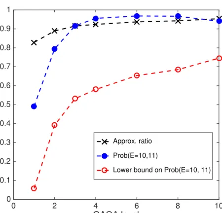
2. Typical solution upon measurements

Note that our optimization over the set of angles is de-signed to maximize the expected value, and the high ap-proximation ratio discussed in Section V C 1 is also about the expected value. For approximate optimization, the expectation value of the approximation ratio is not the whole story. One also cares about the probability of get-ting the optimal or near-optimal states upon measure-ment. We apply the argument and analysis on the tail probability in Sec. II, Eq. (1), on the case of 3-coloring of the Envelope graph (11 edges), and show in Figure 9 the theoretical lower bound in probability of getting a solu-tion with costs 10 or 11, i.e., the valid coloring or only one improperly-colored edges. The true probability from evaluating the wavefunction is shown for comparison. For QAOA level three and up, the bound inferred from the approximation ratio gives us confidence that with greater than 50% probability we will get the optimal or the next best solutions.

Viewing the QAOA as an exact solver, as observed in the case of small hard-to-color graphs, for the bench-marking problem sets, we also see that as p increases, along with the increase in r⇤, there is a more drastic increase in the prob-to-optimal-solution. In Fig. 8 we also plot the mean prob-to-optimal-solution asp changes, with error bars indicating the standard deviation over the graphs in the set.

QAOA level 0 2 4 6 8 10 0 0.1 0.2 0.3 0.4 0.5 0.6 0.7 0.8 0.9 1 Approx. ratio Prob(E=10,11)

Lower bound on Prob(E=10, 11)

Figure 9. 3-coloring of Envelope graph (11 edges). QAOA with simultaneous ring-mixer. For each QAOA level, the probability of getting the top two highest approximate re-sults (cost 11 and 10) is shown in comparison to the bound given by Eq. (1) with the observed approximation ratio as parameter.

3

X _{2 {}0,1, . . . , m_}, if the mean value is µ then for any

l _{ b}µ_c, where _b·c is the floor function, the probability of x taking value larger than l is lower-bounded as

Pr(X > l) µ l

m l . (1)

In Appendix. A we provide a proof for Eq. (1) under more general assumptions. In Sec. V C we will see exam-ples: for our QAOA results of high approximation ratio, without examining the energy distribution, we can in-fer with high confidence that a typical solution will have high cost.

III. PROBLEM FORMULATION

In this section we formulate the Max- -Colorable-Subgraph problem in binary form using a one-hot-encoding representation for the possible colorings of each node. Using binary variable xv,c to indicate whether ver-tex v is assigned color c, the one-hot-encoding formu-lation requires solutions live in a subspace of the full Hilbert space that satisfies: P_c xv,c = 1, the feasible

subspace. This results in two formulations of the

color-ing problem for QAOA–with and without a penalty term in the phase-separator. We also recap nomenclature for various XY -Hamiltonian drivers introduced in Ref. [2] which becomes necessary when discussing their circuit implementations.

The Max--Colorable-Subgraph problem is formulated as follows:

Problem 1. Given a graph G = (V, E) with n vertices

and m edges, and  colors, maximize the size (number of edges) of a properly vertex-colored subgraph.

The max--Colorable-Subgraph problem is encoded into qubits with a one-hot encoding fashion to represent the colors. Each node of the graph G is expanded into 

qubits where each qubit occupation is used to represent a coloring of the node. For example, a three-coloring prob-lem on a graph of 4 vertices requires 12 qubits depicted in Figure 1.

In the feasible subspace where each vertex is assigned exactly one color, the cost/objective function

fC = m  X j=1 X {v,v0_}2E xv,jxv0_,j (2)

counts the properly-colored edges, and we aim at maxi-mizing fC. By the replacement x ! (1 z)/2 in Eq. (2),

the corresponding quantum objective Hamiltonian is

HC = 1 4 ⇣ (4 )m1 + H_C0 ⌘ , (3) where H_C0 = n X v=1 dv  X j=1 z v,j  X j=1 X {v,v0_}2E z v,j vz0_,j . (4)

Figure 1. Left: The original graph to-be colored. Right: The qubit-layout encoding the problem. Each vertex v is repre-sented by  qubits xv,c for c = 1, . . . representing its 

pos-sible colors. The extended graph construction can be thought of taking the graph represented in its natural euclidean space and then augmenting that space with another dimension and replicating the graph  times for each of the colors. The phase separation Hamiltonian are composed of two-qubit operations corresponding to edges on each surface, and the mixing oper-ation are among the qubits in the augmented dimension.

The approximation ratio we will adopt in the following work is the ratio of the expectation value of the cost Hamiltonian, projected onto the feasible subspace, to the true maximal number of correctly colored edges:

r = hPfeasHCPfeasi

Cmax

, (5)

where Pfeas is the projection operator onto the feasible

subspace, and Cmax is the number of edges in the true

max--colorable subgraph. The numerator in Eq. (5) is equivalent to the average number of properly-colored edges measured upon measurement, with the unfeasible output valued zero.

A. Adding penalty in the phase separating

Hamiltonian

The common practice for incorporate constraints is to add a penalty term to the cost function. For the one-hot-encoded problem we define a quadratic penalty to penalize the case that a node is assigned no color or mul-tiple colors fpen = X v (1  X j=1 xv,j)2 (6)

which, up to a constant, corresponds to the penalty Hamiltonian, Hpen = 1 2 X v ⇣ (2 )X j z v,j + X j<j0 z v,j v,jz 0 ⌘ (7) that increases the energy of all states outside the sub-space. The phase-separating Hamiltonian becomes a weighted sum of the cost and the penalty Hamiltonians

HPS = H_C0 ↵Hpen (8)

9

(a) (b)

Figure 3. Numerical results for level 1 QAOA on the problem

of 3-coloring of a triangle graph. (a) using X mixer along

with phase-separating Hamiltonian, Eq. (8) where the penalty

weight is taken to be the numerically determined optimal

value ↵⇤ = 1.7. (b) using the XY mixer with W-state

be-ing the initial state.

the Envelope graph is the smallest hard-to-color graph for the largest-first(LF) sequential method. Note that these classical algorithms are aiming to compute the chromatic number, while in this paper we focus on find-ing the maximal colorable subgraph. Although findfind-ing the max-colorable subgraph could serve as a subroutine for determining chromatic numbers, the chromatic num-ber can also be directly attacked by QAOA using a much more complex mixer.[2] Nevertheless we are not aiming at doing side-by-side comparison of quantum and classi-cal algorithms, and will use these small graphs only as a proof-of-principle demonstration of the QAOA with XY

mixers.

What graphs to color on NISQ era hardware?

•

For a classical algorithm, there is a concept of

smallest

slightly-hard-to-color graph

: applying the algorithm will

sometimes

yield the optimal solution

&

smallest hard-to-color graph:

applying the algorithm

never

yields the optimal

solution

•

Examples

Envelope

Prism

Small & Hard graphs

Figure 4. The two small and hard-to-color graphs: Envelope and Prism. A valid 3-coloring is shown on each graph.

1. Performance of QAOA with the simultaneous ring mixer

With the simultaneous ring mixer, Figure. 5 shows the results for QAOA levels 1 to 6. For each level, the W-state is used as initial state, and stochastic search

(basin-hopping with BFGS) is performed to optimize the expected value of the cost Hamiltonian over the angle sets. The approximation ratio corresponding to the op-timal expectation value is plotted as filled circles. Even at level one, the approximation ratio takes a high value 0.8, and this value quickly approaches 1 as the level

in-creases. Furthermore, for each level, we computed the probability of getting the actual optimal solution (a valid 3-coloring) upon measurement. At level one, this proba-bility is slightly lower than 0.2, and quickly goes above 0.6 at level-3, which implies that repeating the experiment 3 times, one will find a valid coloring with probability

> 0.9.

Figure 5. The Prism graph. Dots are approximation ratios and crosses are the expected probability of getting the opti-mal coloring. For each QAOA level, results are shown at the (sub)optimal angles resulted from a basin-hopping search.

2. E↵ect of initial states

The W-state – as both an even superposition of all fea-sible classical states, and the ground state of the simul-taneous ring mixer – is a natural candidate for the initial state for QAOA. It involves multiple two-qubit gates to prepare. An easier-to-prepare state for each vertex can be defined via a randomly-assigned coloring (feasible but not necessarily optimal), _| Ci, i.e., a randomly drawn bit

string of Hamming weight one. Preparing such a state involves only n single-qubit gates.

We study both initial states for the prism graph with simultaneous ring mixer. For level-1 QAOA, the best achievable optimization ratio (optimized over all angle sets ( , )) for W-state is higher than the classical Ham-ming weight 1 state _{| i}C. Notice that for | iC, the

phase-separating unitary commutes with the density ma-trix of the state, hence has no e↵ect to the state evolu-tion. As a result, the whole circuit for level-1 QAOA is equivalent to applying the mixing unitary followed by measurement. We further simulated higher levels, and in Figure. 6 show the performance of QAOA with the W-state versus a classical W-state as initial W-state. We found that with the classical initial state, the performance of QAOA is significantly lower than using the W-state as

Choice of initial states

Classical initial state: easy to generate

vs

W-state: Better performance

10 QAOA level 0 2 4 6 8 10 12 Ap p ro x im . ra ti o 0.5 0.6 0.7 0.8 0.9

1 Optimal results for the Prism graph

classical initial states W-state

Figure 6. The Prism graph, the expected value of QAOA op-timized over the angle sets. Triangles show the results with W-state as initial states. Circles show the results with a fea-sible classical initial state, averaged over the set of all feafea-sible classical states, the error bar is the standard deviation. For each initial state, optimization over angles are derived from a basin-hopping search.

initial state. Even at level 10, rclassical is still lower than

rW for level-1. Moreover, the approximation ratio with

classical initial state shows a tendency toward satura-tion around level 10 – this could either be the nature of the algorithm, or due to increasing difficulty in find-ing the global optimum in the parameter subspace as the level increases, which poses another practical considera-tion for applicaconsidera-tion. (Note that due to the optimizaconsidera-tion over parameter space for each initial state, the average over classical initial state is not equivalent to prepare the initial state in a mixed state for the ensemble).

Because our simulation is noise-free, due to ergodicity, in the limit of p _{! 1} the optimal performance should be independent of the initial state. But for practical implementation on a near-term hardware where noises accumulates fast with circuit depth, such medium-level QAOA behavior is of high relevance. In Appendix C we survey methods to generate quantum circuits for prepar-ing W-states. It is shown that with certain methods it can be generated with O() CNOT gates. The over-all performance of QAOA will be a tradeo↵ between the extra e↵ort in preparing W-state and the damage that comes with circuit depth.

C. Benchmarking graph sets

To better understand the behavior of these QAOA graph-coloring algorithms, we make use of the sets of all

-chromatic graphs of size n as the benchmarking sets for the XY mixers under consideration. See Table II for the number of instances in each benchmarking set.

n num. graphs 3 5 12 3 6 64 3 7 475 4 6 26 4 7 282 5 7 46 6 7 5 n  num. graphs 4 4 6 4 6 6 4 8 6

Table II. Left: Benchmarking graph sets: each row indicates all -chromatic graphs of size n, and we solve the problem of -coloring of such graphs choosing  = . Right: Bench-marking graph sets II for examining the simultaneous vs par-titioned ring mixers on di↵erent ring sizes: Each row indicates all connected graphs of size n, and we solve the problem of

-coloring of such graphs. Because the total number of qubits is n, which is the limiting factor to the simulation, we limit to small n to see  varying up to 8.

ring 0.85 0.9 0.95 1 com p le te 0.85 0.9 0.95 1

(a) QAOA level-2

ring 0.95 0.96 0.97 0.98 0.99 1 com p le te 0.95 0.96 0.97 0.98 0.99 1 (b) QAOA level-8

Figure 7. QAOA with simultaneous mixers. Performance comparison between ring and complete-graph mixers applied to the same graph coloring problems. The axes show approx-imation ratio achieved using the labeled mixer type. Scat-ter plot shows the results for 4-coloring of all connected chromatic-4 graphs of size n = 7. In (b), for better visi-bility, an outlier data point at (ring = 0.95, complete = 0.9) is not shown in the plot.

1. Approximation ratio and probability-to-optimal-solution Using W-state as the initial state, for simultaneous ring and complete-graph mixers, the mean and median of the approximation ratio as well as the probability-to-optimal-solution is evaluated across problem sets.

The following observations have been made on the typ-ical performance for each problem set.

a. Consistent performance over instances. For all

problem sets, the approximation ratio and the probability-of-optimal-solution curves as a function of

Generalized W-state

: For any number of qubits

superposition of classical states of Hamming-weight 1.

Eigen-state of the XY mixer, an uniform superposition of all feasible classical states

Classical

initial states: random-coloring of the graph

_{Easier to prepare:}

Parameter setting

Our Algorithm

The building block of our algorithm is

W( ) = e i⇡B/nei Ce i⇡B/ne i C ,

where ₂ (0,⇡] is a free parameter. The unitary W( ) is repeatedly applied to the initial state _|s _i for _O(pN) times.

W( ) |+i e i C e i⇡X/n ei C e i⇡X/n · · · |+i e i⇡X/n e i⇡X/n · · · .. . ... ... ... |+_{i e} i⇡X/n _e i⇡X/n · · ·

Zhang Jiang (NASA) arXiv:1702.02577 19th SQuInT 6 / 14

Our Algorithm

The building block of our algorithm is

W

( ) =

e

i

⇡

B

/

n

e

i C

e

i

⇡

B

/

n

e

i C

,

where

₂

(0

,

⇡

] is a free parameter. The unitary

W

( ) is repeatedly

applied to the initial state

_|

s

_i

for

_O

(

p

N

) times.

W

( )

|

+

_i

e

i C

e

i⇡X/n

e

i C

e

i⇡X/n

· · ·

|

+

_i

_e

i⇡X/n

_e

i⇡X/n

· · ·

..

.

..

.

..

.

..

.

|

+

_i

_e

i⇡X/n

_e

i⇡X/n

· · ·

Zhang Jiang (NASA) arXiv:1702.02577 19th SQuInT 6 / 14

QAOA for Grover’s problem

QAOA Circuit for Grover’s Problem

Given an oracle Hamiltonian that encodes an unknown string

u

,

1

C

_u

=

_|

u

_ih

u

_|

,

the aim is to find out

u

using as few as possible queries of

C

_u

.

The output of a QAOA circuit for Grover’s problem is

|

out

i

=

e

i pB

e

i pCu

· · ·

e

i 1B

e

i 1Cu

|

s

i

.

We find a set of parameters

and

, such that

h

u

|

out

i '

1

/

p

2

,

p

_'

⇡

4

p

2

p

N

,

achieving a near-optimal query complexity.

1

_{The string}

_u

_{can be replaced by}

₀

_{= (0}

_,

₀

_{, . . . ,}

_{0) as long as we replace}

_C

u

with

C

0

.

Zhang Jiang (NASA) arXiv:1702.02577 19th SQuInT 5 / 14

Reproduces the

√

N quantum speedup

QAOA for AF ring (MaxCut on a ring)

z x 2: N

•

Anti-Ferromagnetic Chain:

3

Theorem 1.

For QAOA with

p

= 1

, for each edge

_h

uv

_i

,

h

C

uv

i

(

d, e, f

) =

1

2

+

1

4

sin 4 sin (cos

d

₊

_cos

e

₎

1

4

sin

2

_cos

d+e 2f

₍₁

_cos

f

_{2 )(9)}

where

d

+ 1

and

e

+ 1

are the degrees of vertices

u

and

v

, respectively, and

f

is the number of triangles in the

graph containing edge

_h

uv

_i

.

Here we showed that for

p

= 1 the expectation

value of any edge

_h

C

uv

i

depends only on the parameters

(

d, e, f

). Then the overall expectation value

F

(

,

) =

P

(d,e,f)

h

C

uv

i

(

d, e, f

) (

d, e, f

) where the summation is

taken over distinct subgraphs (

d, e, f

) and (

d, e, f

) is the

multiplicity of the subgraph (

d, e, f

), i.e. the number of

times the subgraph appears in

G

. Thus for an arbitrary

graph

F

(

,

) may be e

ffi

ciently computed classically.

For a triangle-free graph of fixed vertex degree

d

+ 1,

i.e.,

f

= 0 in Eq. (

9

). The expectation value reduces to

F

(

,

) =

|

E

|

2

+

|

E

_|

2

sin 4 sin cos

d

_.

₍₁₀₎

with optimal value

F

⇤

= max

,

F

(

,

) =

|

E

_|

2

+

|

E

_|

2

1

p

d

⇣

_d

D

⌘

D/2

(11)

For any such graph, one optimal pair of angles is (

,

) =

(

⇡

/

8

,

arctan(1

/

p

d

)). MaxCut in the case in which all

vertices have degree 2, so the graph is a ring, is called the

Ring of Disagrees. In this case, maximizing (

10

) yields

the optimization ratio 0

.

75 at (

,

) = (

⇡

/

8

,

⇡

/

4), and

for

d

= 2, the ratio is 0

.

692, both reproducing the results

in [

3

].

For an arbitrary triangle-free graph with maximum

vertex degree

D

, the right-hand side of Eq. (

11

) gives

a lower bound to

F

⇤

. We see that even for

p

= 1, QAOA

always beats random guessing.

It is straightforward to extend the analysis to QAOA of

higher levels. The number of such terms quickly becomes

prohibitive for direct calculation, however; many more

non-commuting terms coming from the

U

C

’s and

U

B

’s

must be retained and carried through the calculation.

The expectation value of a given edge will also depend on

its local graph topology (within

p

hops), which becomes

di

ffi

cult to succinctly characterize as

p

increases.

IV. ANALYSIS OF THE PROBLEM OF RING OF DISAGREES (ANTI-FERROMAGNETIC

CHAIN)

We now study in detail QAOA for the ring of disagrees,

where the symmetry and simplicity of the problem means

that analysis can be done for QAOA of arbitrary level

p

.

Numerical results for small

p

, and a conjecture for the

approximation ratio for arbitrary

p

were given in Ref. [

3

].

A. Formulation of the problem

The Hamiltonian for MaxCut on a ring, or the Ring of

Disagrees, with

N

vertices is ˜

H

C

=

1₂

P

N_j=1

(1

_jz _jz₊₁

)

where

_Nz ₊₁

=

₁z

. For convenience, we consider only

even

N

, in which case the ground state of ˜

H

C

is

triv-ial with every pair of neighboring spins aligned in

anti-parallel fashion, corresponding to

F

opt

=

N

.

To simplify the derivation, and without losing

gener-ality, we drop the constant and rescale ˜

H

C

to be

H

C

=

X

j

z

j jz+1

(12)

which is used in the evolution operator Eq. (

2

). Since

the rescaling dropped a negative sign, the maximization

problem becomes a minimization problem. The initial

state of the system is prepared as Eq. (

4

), and the

algo-rithm follows the evolution Eq. (

5

).

The relation between angles, expectation value used in

this paper and the ones in Ref. [

3

] (notations with tilde)

is

=

˜

/

2,

= ˜ and ˜

F

(

˜

,

˜

) =

N

F

(

,

)

/

2

B. Fermionic representation

We show that using a Fermionic representation, the

problem reduces to optimal quantum control of an

en-semble of independent spins (spin-1/2), significantly

sim-plifying the analysis.

We apply the Jordan-Wigner transformation [

1

,

8

],

a

j

=

1

2

( 1)

j 1 y j

+

i

jz j

_Y

1 k=1 x k

(13)

a

†_j

=

1

2

( 1)

j 1 y j

i

jz j

_Y

1 k=1 x k

(14)

where

a

j

, a

†_j

obey the fermionic canonical commutation

relations. Accordingly,

H

C

=

N

_X

1 j=1

a

†_j

a

j+1

+

a

j

a

j+1

(

a

†_N

a

1

+

a

N

a

1

)

G

+ h

.

c

.

(15)

where

we

introduce

the

gauge

operator

G

=

exp[

i

⇡

P

N_l=1

a

†_l

a

l

] = ( 1)

N

Q

N_{j=1 j}x

.

In the current

(standard) QAOA settings, for even

N

, the initial state

is an eigenstate of

G

with eigenvalue 1. The operator

G

is a constant of motion since it commutes with both

H

B

and

H

C

, so the value of

G

remains 1 throughout the

evolution. The sign of the

j

=

N

terms in

H

C

there-fore are di

↵

erent from the others. We further introduce

a phase factor to unify the expression,

b

j

=

a

j

e

ij⇡/N

.

•

Analysis: Jordan-Wigner transformation

for 1D spin chain with n.n. couplings

2-axis control of

N/2 independent

spins with

collective angles

coupled spin

chain of size

N

. . .

^ k z x

γ

β

γ

[Wang, Hadfield, Jiang, Rieffel, QAOA for MaxCut: a fermonic review, PRA 2018] [Jiang, Rieffel, Wang, Near-optimal quantum

circuit for Grover's unstructured search using a transverse field, PRA 2017]

Deterministic parameters:

Rugged landscape — stochastic optimizing is needed

Summary

•

We outlined important aspects of benchmarking quantum heuristics

•

Using QAOA with XY mixer as an example, we demonstrated that influences to

algorithm performance could come from

•

Design principle

— Choice of “Cost function”: challenges the guidance role of energy in QAOA

— Choice of Mixers: contains search in feasible subspace satisfying constraints

— Choice of initial state: tradeoff between good (noise-free) performance and

complexity of state-preparation

•

Implementation on hardware

•

— Circuit-depth for XY gates: can be efficiently implemented on hardware: from

all-to-all to a chain connectivity

•

Parameter setting and Quantum control landscape

From QAOA to QAOA: [Hadfield, Wang, O'Gorman, Rieffel, Venturelli, Biswas, Algorithms 2019]

QAOA for MaxCut: a fermonic view,[Wang, Hadfield, Jiang, Rieffel, PRA 2018]

QAOA for Grover: [Jiang, Rieffel, Wang, PRA 2017] XY mixers for QAOA: [Wang, Rubin,